00footnotetext: To appear in: Communications in Mathematical Sciences.

The Riemann problem for the shallow water equations with discontinuous topography

Philippe G. LeFloch and Mai Duc Thanh Philippe G. LeFloch
Laboratoire Jacques-Louis Lions & Centre National de la Recherche Scientifique, Université de Paris 6, 4 Place Jussieu, 75252 Paris, France.
LeFloch@ann.jussieu.fr Mai Duc Thanh
Department of Mathematics, International University, Quarter 6, Linh Trung Ward, Thu Duc District, Ho Chi Minh City, Vietnam
MDThanh@hcmiu.edu.vn
Abstract.

We construct the solution of the Riemann problem for the shallow water equations with discontinuous topography. The system under consideration is non-strictly hyperbolic and does not admit a fully conservative form, and we establish the existence of two-parameter wave sets, rather than wave curves. The selection of admissible waves is particularly challenging. Our construction is fully explicit, and leads to formulas that can be implemented numerically for the approximation of the general initial-value problem.

Key words and phrases:
Shallow water, conservation law, Riemann problem, discontinuous topography.
2000 Mathematics Subject Classification:
35L65, 76N10, 76L05

1. Introduction

1.1. Shallow water equations

We consider the one-dimensional shallow water equations

th+x(hu)=0,subscript𝑡subscript𝑥𝑢0\displaystyle\partial_{t}h+\partial_{x}(hu)=0, (1.1)
t(hu)+x(h(u2+gh2))=ghxa,subscript𝑡𝑢subscript𝑥superscript𝑢2𝑔2𝑔subscript𝑥𝑎\displaystyle\partial_{t}(hu)+\partial_{x}(h(u^{2}+g\frac{h}{2}))=-gh\partial_{x}a,
ta=0,subscript𝑡𝑎0\displaystyle\partial_{t}a=0,

where hh denotes the height of the water from the bottom to the surface, u𝑢u the velocity of the fluid, g𝑔g the gravity constant, and a𝑎a the height of the river bottom from a given level. Following LeFloch [18] we supplement the first two balance laws for the fluid with the equation ta=0subscript𝑡𝑎0\partial_{t}a=0 corresponding to a fixed geometry. Adding the equation ta=0subscript𝑡𝑎0\partial_{t}a=0 allows us to view the shallow water equations (the first two equations in (1.1)), which form a strictly hyperbolic system of balance laws in nonconservative form, as a non-strictly hyperbolic system of balance laws with a linearly degenerate characteristic field.

We are mainly interested in the case that a𝑎a is piecewise constant

a(x)={aL,x<0,aR,x>0,𝑎𝑥casessubscript𝑎𝐿𝑥0subscript𝑎𝑅𝑥0a(x)=\left\{\begin{array}[]{ll}a_{L},&x<0,\\ a_{R},&x>0,\end{array}\right.

where aL,aRsubscript𝑎𝐿subscript𝑎𝑅a_{L},a_{R} are two distinct constants. The Riemann problem associated with (1.1) is the initial-value problem corresponding to the initial conditions of

(h,u,a)(x,0)={(hL,uL,aL),x<0,(hR,uR,aR),x>0.𝑢𝑎𝑥0casessubscript𝐿subscript𝑢𝐿subscript𝑎𝐿𝑥0subscript𝑅subscript𝑢𝑅subscript𝑎𝑅𝑥0(h,u,a)(x,0)=\left\{\begin{array}[]{ll}(h_{L},u_{L},a_{L}),&x<0,\\ (h_{R},u_{R},a_{R}),&x>0.\end{array}\right. (1.2)

Since a𝑎a is discontinuous, the system (1.1) cannot be written in a fully conservative form, and the standard notion of weak solutions for hyperbolic systems of conservation laws does not apply. However, the equations still make sense within the framework introduced in Dal Maso, LeFloch, and Murat [7]. (For a recent review see [19, 20].)

1.2. DLM generalized Rankine-Hugoniot relations

Consider an elementary discontinuity propagating with the speed λ𝜆\lambda and satisfying the equations (1.1). Observe that the Rankine-Hugoniot relation associated with the third equation in (1.1) simply reads

λ[a]=0,𝜆delimited-[]𝑎0-\lambda[a]=0, (1.3)

where [a]:=a+aassigndelimited-[]𝑎subscript𝑎subscript𝑎[a]:=a_{+}-a_{-} denotes the jump of the bottom level function a𝑎a, and a±subscript𝑎plus-or-minusa_{\pm} denotes its left- and right-hand traces. Then, we have the following possibilities:

  • (i)

    either the component a𝑎a remains constant across the propagating discontinuity,

  • (ii)

    or a𝑎a changes its levels across the discontinuity and the discontinuity is stationary, i.e., the speed λ𝜆\lambda vanishes.

This observation motivates us to define the admissible elementary waves of the system (1.1). First of all, assume that the bottom level a𝑎a remains constant across a discontinuity; then, a𝑎a should be constant in a neighborhood of the discontinuity. Eliminating a𝑎a from (1.1), we obtain the following system of two conservation laws

th+x(hu)=0,subscript𝑡subscript𝑥𝑢0\displaystyle\partial_{t}h+\partial_{x}(hu)=0, (1.4)
t(hu)+x(h(u2+gh2))=0,subscript𝑡𝑢subscript𝑥superscript𝑢2𝑔20\displaystyle\partial_{t}(hu)+\partial_{x}(h(u^{2}+g\frac{h}{2}))=0,

Thus, the left- and right-hand states are related by the Rankine Hugoniot relations corresponding to (1.4)

λ[h]+[hu]=0,𝜆delimited-[]delimited-[]𝑢0\displaystyle-\lambda[h]+[hu]=0, (1.5)
λ[hu]+[h(u2+gh2)]=0,𝜆delimited-[]𝑢delimited-[]superscript𝑢2𝑔20\displaystyle-\lambda[hu]+[h(u^{2}+g\frac{h}{2})]=0,

where [h]:=h+h+assigndelimited-[]subscriptsubscript[h]:=h_{+}-h_{+}, etc.

Second, suppose that the component a𝑎a is discontinuous so that the speed vanishes. Then, the solution is independent of the time variable, and it is natural to search for a solution obtained as the limit of a sequence of time-independent smooth solutions of (1.1). (See below.)

Suppose that (x,t)(h,u,a)maps-to𝑥𝑡𝑢𝑎(x,t)\mapsto(h,u,a) is a smooth solution of (1.1). Then, the system (1.1) can be written in the following form, as a system of conservation laws for the (now conservative) variables (h,u,a)𝑢𝑎(h,u,a):

th+x(hu)=0,subscript𝑡subscript𝑥𝑢0\displaystyle\partial_{t}h+\partial_{x}(hu)=0, (1.6)
tu+x(u22+g(h+a))=0,subscript𝑡𝑢subscript𝑥superscript𝑢22𝑔𝑎0\displaystyle\partial_{t}u+\partial_{x}\big{(}{u^{2}\over 2}+g(h+a)\big{)}=0,
ta=0.subscript𝑡𝑎0\displaystyle\partial_{t}a=0.

Hence, time-independent solutions of (1.1) satisfy

(hu)=0,superscript𝑢0\displaystyle(hu)^{\prime}=0, (1.7)
(u22+g(h+a))=0,superscriptsuperscript𝑢22𝑔𝑎0\displaystyle\big{(}{u^{2}\over 2}+g(h+a)\big{)}^{\prime}=0,

where the dash denotes the differentiation with respect to x𝑥x. Trajectories initiating from a given state (h0,u0,a0)subscript0subscript𝑢0subscript𝑎0(h_{0},u_{0},a_{0}) are given by

hu=h0u0,𝑢subscript0subscript𝑢0\displaystyle hu=h_{0}u_{0}, (1.8)
u22+g(h+a)=u022+g(h0+a0).superscript𝑢22𝑔𝑎superscriptsubscript𝑢022𝑔subscript0subscript𝑎0\displaystyle{u^{2}\over 2}+g(h+a)={u_{0}^{2}\over 2}+g(h_{0}+a_{0}).

It follows from (1.8) that the trajectories of (1.7) can be expressed in the form u=u(h)𝑢𝑢u=u(h), a=a(h)𝑎𝑎a=a(h). Now, letting hh±subscriptplus-or-minush\to h_{\pm} and setting u±=u(h±)subscript𝑢plus-or-minus𝑢subscriptplus-or-minusu_{\pm}=u(h_{\pm}), a±=a(h±)subscript𝑎plus-or-minus𝑎subscriptplus-or-minusa_{\pm}=a(h_{\pm}), we see that the states (h±,u±,a±)subscriptplus-or-minussubscript𝑢plus-or-minussubscript𝑎plus-or-minus(h_{\pm},u_{\pm},a_{\pm}) satisfy the Rankine-Hugoniot relations associated with (1.6), but with zero shock speed:

[hu]=0,delimited-[]𝑢0\displaystyle[hu]=0, (1.9)
[u22+g(h+a)]=0,delimited-[]superscript𝑢22𝑔𝑎0\displaystyle[{u^{2}\over 2}+g(h+a)]=0,

The above discussion leads us to define the elementary waves of interest, as follows.

Definition 1.1.

The admissible waves for the system (1.1) are the following ones:

  • (a)

    the rarefaction waves, which are smooth solutions of (1.1) with constant component a𝑎a depending only on the self-similarity variable x/t𝑥𝑡x/t;

  • (b)

    the shock waves which satisfy (1.5) and Lax shock inequalities and have constant component a𝑎a;

  • (c)

    and the stationary waves which have zero speed and satisfy (1.9).

As will be checked later, the system (1.1) is not strictly hyperbolic, as was already observed in the previous work [21]. Recall that therein we studied the Riemann problem in a nozzle with variable cross-section and constructed all of the Riemann solutions. The present model is analogous, and our main purpose in the present paper is to demonstrate that the technique in [21] extends to the shallow water model and to construct the solution of the Riemann problem. The lack of strict hyperbolicity and the nonconservative form of the equation make the problem particularly challenging. Some aspects of this problem are also covered by Alcrudo and Benkhaldoun [1]. For works on various related models including scalar conservation laws we refer to [22, 15, 14, 13, 12, 9, 8, 2].

1.3. Results and perspectives

As we will show, waves in the same characteristic field may be repeated in a single Riemann solution. This happens when waves cross the boundary of the strictly hyperbolic regions and the order of characteristic speeds changes. We will also show below that the Riemann problem may not always have a solution. The Riemann problem may admit exactly one, or two, or up to three distinct solutions for different ranges of left-hand and right-hand states. Thus, uniqueness does not hold for the Riemann problem, as was already observed for the nozzle flow system.

Each possible construction leads to a solution that depends continuously on the left-hand and right-hand states. This is a direct consequence of the smoothness of the elementary wave curves; by the implicit function theorem, the intermediate waves depend continuously on their left- or right-hand states as well as on the Riemann data. These results agree with [21] which covered fluids in a nozzle with variable cross section.

In the present model, the curve of stationary wave is strictly convex. To find stationary waves, one needs to determine the roots of a nonlinear equation (see the function φ𝜑\varphi in (3.1)) which is convex and, therefore, can be easily computed numerically. The Riemann solver derived in the present paper should be useful in combination with numerical methods for shallow water systems developed in [3, 4, 11, 10, 16, 6] for which we refer to the lecture notes by Bouchut [5].

2. Background

2.1. Shallow water equations as a non-strictly hyperbolic system

We now discuss the system (1.1) in the nonconservative variables U=(h,u,a)𝑈𝑢𝑎U=(h,u,a). From (1.6) if follows that, for smooth solutions, (1.1) is equivalent to

th+uxh+hxu=0,subscript𝑡𝑢subscript𝑥subscript𝑥𝑢0\displaystyle\partial_{t}h+u\partial_{x}h+h\partial_{x}u=0, (2.1)
tu+gxh+uxu+gxa=0,subscript𝑡𝑢𝑔subscript𝑥𝑢subscript𝑥𝑢𝑔subscript𝑥𝑎0\displaystyle\partial_{t}u+g\partial_{x}h+u\partial_{x}u+g\partial_{x}a=0,
ta=0,subscript𝑡𝑎0\displaystyle\partial_{t}a=0,

which can be written in the nonconservative form

tU+A(U)xU=0,subscript𝑡𝑈𝐴𝑈subscript𝑥𝑈0\partial_{t}U+A(U)\partial_{x}U=0, (2.2)

where the Jacobian matrix A(U)𝐴𝑈A(U) is given by

A(U)=(uu0gug000).𝐴𝑈matrix𝑢𝑢0𝑔𝑢𝑔000A(U)=\left(\begin{matrix}u&u&0\\ g&u&g\\ 0&0&0\end{matrix}\right).

The eigenvalues of A𝐴A are

λ1(U):=ugh<λ2(U):=u+gh,λ3(U):=0,formulae-sequenceassignsubscript𝜆1𝑈𝑢𝑔subscript𝜆2𝑈assign𝑢𝑔assignsubscript𝜆3𝑈0\lambda_{1}(U):=u-\sqrt{gh}<\lambda_{2}(U):=u+\sqrt{gh},\quad\lambda_{3}(U):=0, (2.3)

and corresponding eigenvectors can be chosen as

r1(U):=(h,gh,0)t,r2(U):=(h,gh,0)t,formulae-sequenceassignsubscript𝑟1𝑈superscript𝑔0𝑡assignsubscript𝑟2𝑈superscript𝑔0𝑡\displaystyle r_{1}(U):=(h,-\sqrt{gh},0)^{t},\quad r_{2}(U):=(h,\sqrt{gh},0)^{t}, (2.4)
r3(U):=(gh,gu,u2gh)t.assignsubscript𝑟3𝑈superscript𝑔𝑔𝑢superscript𝑢2𝑔𝑡\displaystyle r_{3}(U):=(gh,-gu,u^{2}-gh)^{t}.

We see that the first and the third characteristic fields may coincide:

(λ1(U),r1(U))=(λ3(U),r3(U))subscript𝜆1𝑈subscript𝑟1𝑈subscript𝜆3𝑈subscript𝑟3𝑈(\lambda_{1}(U),r_{1}(U))=(\lambda_{3}(U),r_{3}(U))

on a hypersurface in the variables (h,u,a)𝑢𝑎(h,u,a), which can be identified as

𝒞+:={(h,u,a)|u=gh}.\mathcal{C}_{+}:=\{(h,u,a)|\quad u=\sqrt{gh}\}. (2.5)

Similarly, the second and the third characteristic fields may coincide:

(λ2(U),r2(U))=(λ3(U),r3(U))subscript𝜆2𝑈subscript𝑟2𝑈subscript𝜆3𝑈subscript𝑟3𝑈(\lambda_{2}(U),r_{2}(U))=(\lambda_{3}(U),r_{3}(U))

on a hypersurface in the variables (h,u,a)𝑢𝑎(h,u,a), which can be identified as

𝒞:={(h,u,a)|u=gh}.\mathcal{C}_{-}:=\{(h,u,a)|\quad u=-\sqrt{gh}\}. (2.6)

The third eigenvalue (λ3,r3)subscript𝜆3subscript𝑟3(\lambda_{3},r_{3}) is linearly degenerate, and we have

λ1(U)r1(U)=λ2(U)r2(U)=32gh0,h>0.formulae-sequencesubscript𝜆1𝑈subscript𝑟1𝑈subscript𝜆2𝑈subscript𝑟2𝑈32𝑔00-\nabla\lambda_{1}(U)\cdot r_{1}(U)=\nabla\lambda_{2}(U)\cdot r_{2}(U)={3\over 2}\sqrt{gh}\neq 0,\quad h>0.

Note also that the first and the second characteristic fields (λ1,r1)subscript𝜆1subscript𝑟1(\lambda_{1},r_{1}), (λ2,r2)subscript𝜆2subscript𝑟2(\lambda_{2},r_{2}) are genuinely nonlinear in the open half-space {(h,u,a)|h>0}\{(h,u,a)|\quad h>0\}.

It is convenient to set

𝒞=𝒞+𝒞={(h,u,a)|u2gh=0},\mathcal{C}=\mathcal{C}_{+}\cup\mathcal{C}_{-}=\{(h,u,a)|\quad u^{2}-gh=0\},

which is the hypersurface on which the system fails to be strictly hyperbolic.

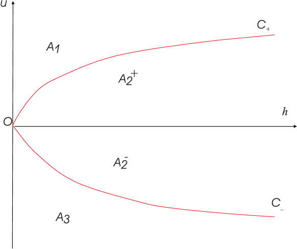
In conclusion we have established (cf. Figure 1):

Lemma 2.1.

On the hypersurface 𝒞+subscript𝒞\mathcal{C}_{+} in the variables (h,u,a)𝑢𝑎(h,u,a) the first and the third characteristic speeds coincide and, on the hypersurface 𝒞subscript𝒞\mathcal{C}_{-}, the second and the third characteristic speeds coincide. Hence, the system (1.1) is non-strictly hyperbolic.
Refer to caption
Figure 1. Projection of strictly hyperbolic regions in the (h,u)𝑢(h,u)-plane

The hypersurface 𝒞𝒞\mathcal{C} divides the phase domain into three disjoint regions, denoted by A1,A2subscript𝐴1subscript𝐴2A_{1},A_{2} and A3subscript𝐴3A_{3}, in which the system is strictly hyperbolic. More precisely, we define

A1:={(h,u,a)RI+×RI×RI+|λ2(U)>λ1(U)>λ3(U)},\displaystyle A_{1}:=\{(h,u,a)\in{R\!\!\!\!\!I~{}}_{+}\times{R\!\!\!\!\!I~{}}\times{R\!\!\!\!\!I~{}}_{+}|\quad\lambda_{2}(U)>\lambda_{1}(U)>\lambda_{3}(U)\}, (2.7)
A2:={(h,u,a)RI+×RI×RI+|λ2(U)>λ3(U)>λ1(U)},\displaystyle A_{2}:=\{(h,u,a)\in{R\!\!\!\!\!I~{}}_{+}\times{R\!\!\!\!\!I~{}}\times{R\!\!\!\!\!I~{}}_{+}|\quad\lambda_{2}(U)>\lambda_{3}(U)>\lambda_{1}(U)\},
A2+:={(h,u,a)A2|u>0},\displaystyle A_{2}^{+}:=\{(h,u,a)\in A_{2}|\quad u>0\},
A2:={(h,u,a)A2|u<0},\displaystyle A_{2}^{-}:=\{(h,u,a)\in A_{2}|\quad u<0\},
A3:={(h,u,a)RI+×RI×RI+|λ3(U)>λ2(U)>λ1(U)}.\displaystyle A_{3}:=\{(h,u,a)\in{R\!\!\!\!\!I~{}}_{+}\times{R\!\!\!\!\!I~{}}\times{R\!\!\!\!\!I~{}}_{+}|\quad\lambda_{3}(U)>\lambda_{2}(U)>\lambda_{1}(U)\}.

The strict hyperbolicity domain is not connected, which makes the Riemann problem delicate to solve.

2.2. Wave curves

We begin by investigating some properties of the curves of admissible waves.

First, consider shock curves from a given left-hand state U0=(h0,u0,a0)subscript𝑈0subscript0subscript𝑢0subscript𝑎0U_{0}=(h_{0},u_{0},a_{0}) consisting of all right-hand states U=(h,u,a)𝑈𝑢𝑎U=(h,u,a) that can be connected to U0subscript𝑈0U_{0} by a shock wave. Thus, it follows from (1.6) that U𝑈U and U0subscript𝑈0U_{0} are related by the Rankine-Hugoniot relations

λ¯[h]+[hu]=0,¯𝜆delimited-[]delimited-[]𝑢0\displaystyle-\bar{\lambda}[h]+[hu]=0, (2.8)
λ¯[hu]+[h(u2+gh2]=0,\displaystyle-\bar{\lambda}[hu]+[h(u^{2}+g\frac{h}{2}]=0,

where [h]=hh0delimited-[]subscript0[h]=h-h_{0}, etc, and λ¯=λ¯(U0,U)¯𝜆¯𝜆subscript𝑈0𝑈\bar{\lambda}=\bar{\lambda}(U_{0},U) is the shock speed.

Fix the state U0subscript𝑈0U_{0}. A straightforward calculation from the Rankine-Hugoniot relations (2.8) shows that the restriction to the (h,u)𝑢(h,u) plane of the Hugoniot set consists of two curves given by

u=u0±g2(hh0)(1h+1h0).𝑢plus-or-minussubscript𝑢0𝑔2subscript011subscript0u=u_{0}\pm\sqrt{g\over 2}(h-h_{0})\sqrt{\Big{(}{1\over h}+{1\over h_{0}}\Big{)}}. (2.9)

Moreover, along these two curves it holds

dudh𝑑𝑢𝑑\displaystyle{du\over dh} =±g2(1h+1h0(hh0)12h21h+1h0)absentplus-or-minus𝑔211subscript0subscript012superscript211subscript0\displaystyle=\pm\sqrt{g\over 2}\Big{(}\sqrt{{1\over h}+{1\over h_{0}}}-(h-h_{0}){1\over 2h^{2}\sqrt{\dfrac{1}{h}+\dfrac{1}{h_{0}}}}\Big{)}
±gh0 as hh0.absentplus-or-minus𝑔subscript0 as hh0.\displaystyle\to\pm\sqrt{g\over h_{0}}\text{ as $h\to h_{0}$.}

Since the i𝑖ith-Hugoniot curve is tangent to ri(U0)subscript𝑟𝑖subscript𝑈0r_{i}(U_{0}) at U0subscript𝑈0U_{0}, we conclude that the first Hugoniot curve associated with the first characteristic field is

1(U0):u:=u1(h,U0)=u0g2(hh0)(1h+1h0),h0,\mathcal{H}_{1}(U_{0}):\quad u:=u_{1}(h,U_{0})=u_{0}-\sqrt{g\over 2}(h-h_{0})\sqrt{\Big{(}{1\over h}+{1\over h_{0}}\Big{)}},\quad h\geq 0, (2.10)

while one associated with the second characteristic field is

2(U0):u:=u2(h,U0)=u0+g2(hh0)(1h+1h0),h0.\mathcal{H}_{2}(U_{0}):\quad u:=u_{2}(h,U_{0})=u_{0}+\sqrt{g\over 2}(h-h_{0})\sqrt{\Big{(}{1\over h}+{1\over h_{0}}\Big{)}},\quad h\geq 0. (2.11)

Along the Hugoniot curves 1,2subscript1subscript2\mathcal{H}_{1},\mathcal{H}_{2}, the corresponding shock speeds are given by

λ¯1,2(U0,U)subscript¯𝜆12subscript𝑈0𝑈\displaystyle\bar{\lambda}_{1,2}(U_{0},U) =hu1,2h0u0hh0absentsubscript𝑢12subscript0subscript𝑢0subscript0\displaystyle={hu_{1,2}-h_{0}u_{0}\over h-h_{0}} (2.12)
=u0g2(h+h2h0),h0,formulae-sequenceabsentminus-or-plussubscript𝑢0𝑔2superscript2subscript00\displaystyle=u_{0}\mp\sqrt{{g\over 2}\Big{(}h+{h^{2}\over h_{0}}\Big{)}},\quad h\geq 0,

As is customary, the shock speed λ¯i(U0,U)subscript¯𝜆𝑖subscript𝑈0𝑈\bar{\lambda}_{i}(U_{0},U) is required to satisfy Lax shock inequalities [17]:

λi(U)<λ¯i(U0,U)<λi(U0),i=1,2.formulae-sequencesubscript𝜆𝑖𝑈subscript¯𝜆𝑖subscript𝑈0𝑈subscript𝜆𝑖subscript𝑈0𝑖12\lambda_{i}(U)<\bar{\lambda}_{i}(U_{0},U)<\lambda_{i}(U_{0}),\quad i=1,2. (2.13)

Thus, the 111-shock curve 𝒮1(U0)subscript𝒮1subscript𝑈0\mathcal{S}_{1}(U_{0}) initiating from the left-hand state U0subscript𝑈0U_{0} and consisting of all right-hand states U𝑈U that can be connected to U0subscript𝑈0U_{0} by a Lax shock associated with the first characteristic field is

𝒮1(U0):u=u1(h,U0)=u0g2(hh0)(1h+1h0),h>h0.\mathcal{S}_{1}(U_{0}):\quad u=u_{1}(h,U_{0})=u_{0}-\sqrt{g\over 2}(h-h_{0})\sqrt{\Big{(}{1\over h}+{1\over h_{0}}\Big{)}},\quad h>h_{0}. (2.14)

Similarly, the 222-shock curve 𝒮2(U0)subscript𝒮2subscript𝑈0\mathcal{S}_{2}(U_{0}) issuing from a left-hand state U0subscript𝑈0U_{0} consisting of all right-hand states U𝑈U that can be connected to U0subscript𝑈0U_{0} by a Lax shock associated with the second characteristic field is

𝒮2(U0):u=u1(h,U0)=u0+g2(hh0)(1h+1h0),h<h0,\mathcal{S}_{2}(U_{0}):\quad u=u_{1}(h,U_{0})=u_{0}+\sqrt{g\over 2}(h-h_{0})\sqrt{\Big{(}{1\over h}+{1\over h_{0}}\Big{)}},\quad h<h_{0}, (2.15)

We summarize these results in the following proposition.

Lemma 2.2 (Shock wave curves).

Given a left-hand state U0subscript𝑈0U_{0}, the 111-shock curve 𝒮1(U0)subscript𝒮1subscript𝑈0\mathcal{S}_{1}(U_{0}) consisting of all right-hand states U𝑈U that can be connected to U0subscript𝑈0U_{0} by a Lax shock is

𝒮1(U0):u=u1(h,U0)=u0g2(hh0)(1h+1h0),h>h0.\mathcal{S}_{1}(U_{0}):\quad u=u_{1}(h,U_{0})=u_{0}-\sqrt{g\over 2}(h-h_{0})\sqrt{\Big{(}{1\over h}+{1\over h_{0}}\Big{)}},\quad h>h_{0}.

The 222-shock curve 𝒮2(U0)subscript𝒮2subscript𝑈0\mathcal{S}_{2}(U_{0}) consisting of all right-hand states U𝑈U that can be connected to U0subscript𝑈0U_{0} by a Lax shock is

𝒮2(U0):u=u1(h,U0)=u0+g2(hh0)(1h+1h0),h<h0.\mathcal{S}_{2}(U_{0}):\quad u=u_{1}(h,U_{0})=u_{0}+\sqrt{g\over 2}(h-h_{0})\sqrt{\Big{(}{1\over h}+{1\over h_{0}}\Big{)}},\quad h<h_{0}.

In view of the Lax shock inequalities (2.13), we also conclude that the backward 111-shock curve 𝒮1B(U0)superscriptsubscript𝒮1𝐵subscript𝑈0\mathcal{S}_{1}^{B}(U_{0}) issuing from a right-hand state U0subscript𝑈0U_{0} and consisting of all left-hand states U𝑈U that can be connected to U0subscript𝑈0U_{0} by a Lax shock associated with the first characteristic field is

𝒮1B(U0):u=u1(h,U0)=u0g2(hh0)(1h+1h0),h<h0,\mathcal{S}_{1}^{B}(U_{0}):\quad u=u_{1}(h,U_{0})=u_{0}-\sqrt{g\over 2}(h-h_{0})\sqrt{\Big{(}{1\over h}+{1\over h_{0}}\Big{)}},\quad h<h_{0}, (2.16)

Similarly, the backward 222-shock curve 𝒮2B(U0)superscriptsubscript𝒮2𝐵subscript𝑈0\mathcal{S}_{2}^{B}(U_{0}) issuing from a right-hand state U0subscript𝑈0U_{0} and consisting of all left-hand states U𝑈U that can be connected to U0subscript𝑈0U_{0} by a Lax shock associated with the second characteristic field is

𝒮2B(U0):u=u1(h,U0)=u0+g2(hh0)(1h+1h0),h>h0,\mathcal{S}_{2}^{B}(U_{0}):\quad u=u_{1}(h,U_{0})=u_{0}+\sqrt{g\over 2}(h-h_{0})\sqrt{\Big{(}{1\over h}+{1\over h_{0}}\Big{)}},\quad h>h_{0}, (2.17)

Next, we discuss the properties of rarefaction waves, i.e., smooth self-similar solutions to the system (1.1) associated with one of the two genuinely nonlinear characteristic fields. These waves satisfy the ordinary differential equation:

dUdξ=ri(U)λiri(U),ξ=x/t,i=1,2.formulae-sequence𝑑𝑈𝑑𝜉subscript𝑟𝑖𝑈subscript𝜆𝑖subscript𝑟𝑖𝑈formulae-sequence𝜉𝑥𝑡𝑖12\frac{dU}{d\xi}=\frac{r_{i}(U)}{\nabla\lambda_{i}\cdot r_{i}(U)},\quad\xi=x/t,\quad i=1,2. (2.18)

For waves in the first family, we have

dh(ξ)dξ𝑑𝜉𝑑𝜉\displaystyle\frac{dh(\xi)}{d\xi} =2h(ξ)3gh(ξ)=23gh(ξ),absent2𝜉3𝑔𝜉23𝑔𝜉\displaystyle=-\frac{2h(\xi)}{3\sqrt{gh(\xi)}}=-{2\over 3\sqrt{g}}\sqrt{h(\xi)},
du(ξ)dξ𝑑𝑢𝜉𝑑𝜉\displaystyle\frac{du(\xi)}{d\xi} =2gh(ξ)3gh(ξ)=23,absent2𝑔𝜉3𝑔𝜉23\displaystyle=\frac{-2\sqrt{gh(\xi)}}{-3\sqrt{gh(\xi)}}={2\over 3},
da(ξ)dξ𝑑𝑎𝜉𝑑𝜉\displaystyle\frac{da(\xi)}{d\xi} =0.absent0\displaystyle=0.

It follows that

dudh=gh,𝑑𝑢𝑑𝑔\frac{du}{dh}=-\sqrt{\frac{g}{h}},

therefore, the integral curve passing through a given point U0=(h0,u0,a0)subscript𝑈0subscript0subscript𝑢0subscript𝑎0U_{0}=(h_{0},u_{0},a_{0}) is given by

u=u02g(hh0).𝑢subscript𝑢02𝑔subscript0u=u_{0}-2\sqrt{g}(\sqrt{h}-\sqrt{h_{0}}).

Moreover, the characteristic speed should increase through a rarefaction fan, i.e.,

λ1(U)λ1(U0),subscript𝜆1𝑈subscript𝜆1subscript𝑈0\lambda_{1}(U)\geq\lambda_{1}(U_{0}), (2.19)

which implies

hh0,subscript0h\geq h_{0},

Thus, we define a rarefaction curve 1(U0)subscript1subscript𝑈0\mathcal{R}_{1}(U_{0}) issuing from a given left-hand state U0subscript𝑈0U_{0} and consisting of all the right-hand states U𝑈U that can be connected to U0subscript𝑈0U_{0} by a rarefaction wave associated with the first characteristic field as

1(U0):u=v1(h,U0):=u02g(hh0),hh0.\mathcal{R}_{1}(U_{0}):\quad u=v_{1}(h,U_{0}):=u_{0}-2\sqrt{g}(\sqrt{h}-\sqrt{h_{0}}),\quad h\leq h_{0}. (2.20)

A 111-rarefaction wave is determined by

u=u0+23(xtx0t0)𝑢subscript𝑢023𝑥𝑡subscript𝑥0subscript𝑡0u=u_{0}+{2\over 3}\Big{(}{x\over t}-{x_{0}\over t_{0}}\Big{)} (2.21)

while hh is determined by the equation (2.20) and the component a𝑎a remains constant.

Similarly, we define the rarefaction curve 2(U0)subscript2subscript𝑈0\mathcal{R}_{2}(U_{0}) issuing from a given left-hand state U0subscript𝑈0U_{0} and consisting of all the right-hand states U𝑈U that can be connected to U0subscript𝑈0U_{0} by a rarefaction wave associated with the second characteristic field as

2(U0):u=v2(h,U0):=u0+2g(hh0),hh0.\mathcal{R}_{2}(U_{0}):\quad u=v_{2}(h,U_{0}):=u_{0}+2\sqrt{g}(\sqrt{h}-\sqrt{h_{0}}),\quad h\geq h_{0}. (2.22)

The u𝑢u-component of the 222-rarefaction wave is determined by (2.21) and the hh-component is given by (2.22).

We can summarize the above results in:

Lemma 2.3 (Rarefaction wave curves).

Given a left-hand state U0subscript𝑈0U_{0}, the 111-rarefaction curve 1(U0)subscript1subscript𝑈0\mathcal{R}_{1}(U_{0}) consisting of all right-hand states U𝑈U that can be connected to U0subscript𝑈0U_{0} by a rarefaction wave associated with the first characteristic field is

1(U0):u=v1(h,U0):=u02g(hh0),hh0.\mathcal{R}_{1}(U_{0}):\quad u=v_{1}(h,U_{0}):=u_{0}-2\sqrt{g}(\sqrt{h}-\sqrt{h_{0}}),\quad h\leq h_{0}.

The 222-rarefaction curve 2(U0)subscript2subscript𝑈0\mathcal{R}_{2}(U_{0}) consisting of all right-hand states U𝑈U that can be connected to U0subscript𝑈0U_{0} by a rarefaction wave associated with the second characteristic field is

2(U0):u=v2(h,U0):=u0+2g(hh0),hh0.\mathcal{R}_{2}(U_{0}):\quad u=v_{2}(h,U_{0}):=u_{0}+2\sqrt{g}(\sqrt{h}-\sqrt{h_{0}}),\quad h\geq h_{0}.

We will also need backward curves which we define here for completeness. Given a right-hand state U0subscript𝑈0U_{0}, the 111-rarefaction curve 1B(U0)superscriptsubscript1𝐵subscript𝑈0\mathcal{R}_{1}^{B}(U_{0}) consisting of all left-hand states U𝑈U that can be connected to U0subscript𝑈0U_{0} by a rarefaction wave associated with the first characteristic field is

1B(U0):u=v1(h,U0):=u02g(hh0),hh0.\mathcal{R}_{1}^{B}(U_{0}):\quad u=v_{1}(h,U_{0}):=u_{0}-2\sqrt{g}(\sqrt{h}-\sqrt{h_{0}}),\quad h\geq h_{0}. (2.23)

The 222-rarefaction curve 2B(U0)superscriptsubscript2𝐵subscript𝑈0\mathcal{R}_{2}^{B}(U_{0}) consisting of all left-hand states U𝑈U that can be connected to U0subscript𝑈0U_{0} by a rarefaction wave associated with the second characteristic field is

2B(U0):u=v2(h,U0):=u0+2g(hh0),hh0.\mathcal{R}_{2}^{B}(U_{0}):\quad u=v_{2}(h,U_{0}):=u_{0}+2\sqrt{g}(\sqrt{h}-\sqrt{h_{0}}),\quad h\leq h_{0}. (2.24)

In turn, we are in a position to define the wave curves, as follows

𝒲1(U0)=𝒮1(U0)1(U0),subscript𝒲1subscript𝑈0subscript𝒮1subscript𝑈0subscript1subscript𝑈0\displaystyle\mathcal{W}_{1}(U_{0})=\mathcal{S}_{1}(U_{0})\cup\mathcal{R}_{1}(U_{0}), (2.25)
𝒲1B(U0)=𝒮1B(U0)1B(U0),superscriptsubscript𝒲1𝐵subscript𝑈0superscriptsubscript𝒮1𝐵subscript𝑈0superscriptsubscript1𝐵subscript𝑈0\displaystyle\mathcal{W}_{1}^{B}(U_{0})=\mathcal{S}_{1}^{B}(U_{0})\cup\mathcal{R}_{1}^{B}(U_{0}),
𝒲2(U0)=𝒮2(U0)2(U0),subscript𝒲2subscript𝑈0subscript𝒮2subscript𝑈0subscript2subscript𝑈0\displaystyle\mathcal{W}_{2}(U_{0})=\mathcal{S}_{2}(U_{0})\cup\mathcal{R}_{2}(U_{0}),
𝒲2B(U0)=𝒮2B(U0)2B(U0).superscriptsubscript𝒲2𝐵subscript𝑈0superscriptsubscript𝒮2𝐵subscript𝑈0superscriptsubscript2𝐵subscript𝑈0\displaystyle\mathcal{W}_{2}^{B}(U_{0})=\mathcal{S}_{2}^{B}(U_{0})\cup\mathcal{R}_{2}^{B}(U_{0}).

Some properties of the wave curves are now checked.

Lemma 2.4 (Monotonicity properties).

The wave curve 𝒲1(U0)subscript𝒲1subscript𝑈0\mathcal{W}_{1}(U_{0}) can be parameterized in the form hu=u(h),h>0formulae-sequencemaps-to𝑢𝑢0h\mapsto u=u(h),{h>0}, where the function u𝑢u is strictly convex and strictly decreasing in hh. The wave curve 𝒲2(U0)subscript𝒲2subscript𝑈0\mathcal{W}_{2}(U_{0}) can be parameterized in the form hu=u(h),h>0,formulae-sequencemaps-to𝑢𝑢0h\mapsto u=u(h),h>0, where the function u𝑢u is strictly concave and strictly decreasing in hh.

Proof.

We only give the proof for the 111-wave curve 𝒲1(U0)subscript𝒲1subscript𝑈0\mathcal{W}_{1}(U_{0}), the proof for 𝒲2(U0)subscript𝒲2subscript𝑈0\mathcal{W}_{2}(U_{0}) being similar. For the shock part 𝒮1(U0)subscript𝒮1subscript𝑈0\mathcal{S}_{1}(U_{0}), we have

dudh=g212h+1h0+h02h21h+1h0<0.𝑑𝑢𝑑𝑔2121subscript0subscript02superscript211subscript00{du\over dh}=-\sqrt{g\over 2}\dfrac{\dfrac{1}{2h}+\dfrac{1}{h_{0}}+\dfrac{h_{0}}{2h^{2}}}{\sqrt{\dfrac{1}{h}+\dfrac{1}{h_{0}}}}<0.

For the rarefaction part 1(U0)subscript1subscript𝑈0\mathcal{R}_{1}(U_{0}), we have

dudh=gh<0.𝑑𝑢𝑑𝑔0{du\over dh}=-\sqrt{g\over h}<0.

This establishes the desired monotonicity property of 𝒲1(U0)subscript𝒲1subscript𝑈0\mathcal{W}_{1}(U_{0}).

The convexity of 𝒲1(U)subscript𝒲1𝑈\mathcal{W}_{1}(U) follows from the fact that du/dh𝑑𝑢𝑑du/dh is increasing. Indeed, along the shock part 𝒮1(U0)subscript𝒮1subscript𝑈0\mathcal{S}_{1}(U_{0}) it holds

d2udh2=g2(12h2+h0h3)1h+1h0+12h21h+1h0(12h+1h0+h02h2)1h+1h0>0superscript𝑑2𝑢𝑑superscript2𝑔212superscript2subscript0superscript311subscript012superscript211subscript0121subscript0subscript02superscript211subscript00{d^{2}u\over dh^{2}}=\sqrt{g\over 2}\dfrac{\Big{(}{1\over 2h^{2}}+{h_{0}\over h^{3}}\Big{)}\sqrt{{1\over h}+{1\over h_{0}}}+{1\over 2h^{2}\sqrt{{1\over h}+{1\over h_{0}}}}\Big{(}{1\over 2h}+{1\over h_{0}}+{h_{0}\over 2h^{2}}\Big{)}}{{1\over h}+{1\over h_{0}}}>0

and, along the rarefaction part 1(U0)subscript1subscript𝑈0\mathcal{R}_{1}(U_{0}),

d2udh2=g2h3/2>0,superscript𝑑2𝑢𝑑superscript2𝑔2superscript320{d^{2}u\over dh^{2}}={\sqrt{g}\over 2h^{3/2}}>0,

which completes the proof. \scriptstyle\square

Next, we consider the 333-curve from a state U0subscript𝑈0U_{0}, which consists of all states U𝑈U that can be connected to U0subscript𝑈0U_{0} by a stationary wave. As seen in (1.9), U𝑈U and U0subscript𝑈0U_{0} are related by the Rankine-Hugoniot relations

[hu]=0delimited-[]𝑢0\displaystyle[hu]=0 (2.26)
[u22+g(h+a)]=0.delimited-[]superscript𝑢22𝑔𝑎0\displaystyle[{u^{2}\over 2}+g(h+a)]=0.

This leads to a natural definition of a curve parameterized in hh:

𝒲3(U0):{u=u(h)=h0u0h,a=a(h)=a0+u2u022g+hh0.\mathcal{W}_{3}(U_{0}):\quad\begin{cases}&u=u(h)={h_{0}u_{0}\over h},\\ &a=a(h)=a_{0}+{u^{2}-u_{0}^{2}\over 2g}+h-h_{0}.\end{cases} (2.27)

3. Admissibility conditions for stationary waves

3.1. Two possible stationary jumps

In view of the discussion in the previous section, the states across a stationary wave are constraint by the Rankine-Hugoniot relations (2.26). From a given left-hand state we have to determine the right-hand state, which has three components, determined by the two equations (2.26). Moreover, since the component a𝑎a changes only through stationary waves (which propagate with zero speed) for given bottom levels a±subscript𝑎plus-or-minusa_{\pm} we should solve for u𝑢u and hh in terms of a𝑎a. Thus, we rewrite (2.26) in the form

u=h0u0h,𝑢subscript0subscript𝑢0\displaystyle u={h_{0}u_{0}\over h},
a0a+u2u022g+hh0=0.subscript𝑎0𝑎superscript𝑢2superscriptsubscript𝑢022𝑔subscript00\displaystyle a_{0}-a+{u^{2}-u_{0}^{2}\over 2g}+h-h_{0}=0.

Substituting for u𝑢u and re-arranging the terms, we obtain

u=h0u0h,𝑢subscript0subscript𝑢0\displaystyle u={h_{0}u_{0}\over h},
a0a+u022g(h02h21)+hh0=0.subscript𝑎0𝑎superscriptsubscript𝑢022𝑔superscriptsubscript02superscript21subscript00\displaystyle a_{0}-a+{u_{0}^{2}\over 2g}\Big{(}{h_{0}^{2}\over h^{2}}-1\Big{)}+h-h_{0}=0.

This leads us to search for roots of the function

φ(h):=a0a+u022g(h02h21)+hh0.assign𝜑subscript𝑎0𝑎superscriptsubscript𝑢022𝑔superscriptsubscript02superscript21subscript0\varphi(h):=a_{0}-a+{u_{0}^{2}\over 2g}\Big{(}{h_{0}^{2}\over h^{2}}-1\Big{)}+h-h_{0}. (3.1)

Let us set

hmin(U0):=(u02h02g)1/3,assignsubscriptsubscript𝑈0superscriptsuperscriptsubscript𝑢02superscriptsubscript02𝑔13\displaystyle h_{\min}(U_{0}):=\Big{(}{u_{0}^{2}h_{0}^{2}\over g}\Big{)}^{1/3}, (3.2)
amin(U0):=a0+u022g(h02hmin21)+hminh0.assignsubscript𝑎subscript𝑈0subscript𝑎0superscriptsubscript𝑢022𝑔superscriptsubscript02superscriptsubscript21subscriptsubscript0\displaystyle a_{\min}(U_{0}):=a_{0}+{u_{0}^{2}\over 2g}\Big{(}{h_{0}^{2}\over h_{\min}^{2}}-1\Big{)}+h_{\min}-h_{0}.

Some useful properties of the function φ𝜑\varphi in (3.1) are now derived.

Lemma 3.1.

Suppose that U0=(h0,u0,a0)subscript𝑈0subscript0subscript𝑢0subscript𝑎0U_{0}=(h_{0},u_{0},a_{0}) and a𝑎a are given with u00subscript𝑢00u_{0}\neq 0. The function φ:(0,+)RI:𝜑0𝑅𝐼\varphi:(0,+\infty)\to{R\!\!\!\!\!I~{}} is smooth and convex and, for some hminsubscripth_{\min}, it is decreasing in the interval (0,hmin)0subscript(0,h_{\min}) and is increasing in the interval (hmin,)subscript(h_{\min},\infty), with

limh0φ(h)=limh+φ(h)=+.subscript0𝜑subscript𝜑\lim_{h\to 0}\varphi(h)=\lim_{h\to+\infty}\varphi(h)=+\infty. (3.3)

Furthermore, if aamin𝑎subscript𝑎a\geq a_{\min} then the function φ𝜑\varphi has two roots h(U0),h(U0)subscriptsubscript𝑈0superscriptsubscript𝑈0h_{*}(U_{0}),h^{*}(U_{0}) with h(U0)hmin(U0)h(U0)subscriptsubscript𝑈0subscriptsubscript𝑈0superscriptsubscript𝑈0h_{*}(U_{0})\leq h_{\min}(U_{0})\leq h^{*}(U_{0}). These inequalities are strict whenever a>amin(U0)𝑎subscript𝑎subscript𝑈0a>a_{\min}(U_{0}).

Proof.

The smoothness of the function φ𝜑\varphi and the limiting conditions are obvious. Moreover, we have

dφ(h)dh=u02h02gh3+1𝑑𝜑𝑑superscriptsubscript𝑢02superscriptsubscript02𝑔superscript31{d\varphi(h)\over dh}=-{u_{0}^{2}h_{0}^{2}\over gh^{3}}+1

(for u00subscript𝑢00u_{0}\neq 0) which is positive if and only if

h>(u02h02g)1/3=hmin(U0).superscriptsuperscriptsubscript𝑢02superscriptsubscript02𝑔13subscriptsubscript𝑈0h>\Big{(}{u_{0}^{2}h_{0}^{2}\over g}\Big{)}^{1/3}=h_{\min}(U_{0}).

This establishes the monotonicity property of φ𝜑\varphi. Furthermore, we have

d2φ(h)dh2=3u02h02gh40,superscript𝑑2𝜑𝑑superscript23superscriptsubscript𝑢02superscriptsubscript02𝑔superscript40{d^{2}\varphi(h)\over dh^{2}}={3u_{0}^{2}h_{0}^{2}\over gh^{4}}\geq 0,

which shows the convexity of φ𝜑\varphi. If a>amin(U0)𝑎subscript𝑎subscript𝑈0a>a_{\min}(U_{0}), then φ(hmin(U0))<0𝜑subscriptsubscript𝑈00\varphi(h_{\min}(U_{0}))<0. The other conclusions follow immediately. \scriptstyle\square

It is straightforward to check:

Lemma 3.2.

The function hminsubscripth_{\min} satisfies the following inequalities:

hmin(U0)>h0,U0A1A3,formulae-sequencesubscriptsubscript𝑈0subscript0subscript𝑈0subscript𝐴1subscript𝐴3\displaystyle h_{\min}(U_{0})>h_{0},\quad\quad U_{0}\in A_{1}\cup A_{3}, (3.4)
hmin(U0)<h0,U0A2,formulae-sequencesubscriptsubscript𝑈0subscript0subscript𝑈0subscript𝐴2\displaystyle h_{\min}(U_{0})<h_{0},\quad\quad U_{0}\in A_{2},
hmin(U0)=h0,U0𝒞,formulae-sequencesubscriptsubscript𝑈0subscript0subscript𝑈0𝒞\displaystyle h_{\min}(U_{0})=h_{0},\quad\quad U_{0}\in\mathcal{C},

The roots hsuperscripth^{*} and hsubscripth_{*} satisfy the following inequalities:

  • (i)

    If a>a0𝑎subscript𝑎0a>a_{0}, then

    h(U0)<h0<h(U0).subscriptsubscript𝑈0subscript0superscriptsubscript𝑈0h_{*}(U_{0})<h_{0}<h^{*}(U_{0}). (3.5)
  • (ii)

    If a<a0𝑎subscript𝑎0a<a_{0}, then

    h0<h(U0)U0A1A3,formulae-sequencesubscript0subscriptsubscript𝑈0subscript𝑈0subscript𝐴1subscript𝐴3\displaystyle h_{0}<h_{*}(U_{0})\quad\quad U_{0}\in A_{1}\cup A_{3}, (3.6)
    h0>h(U0)U0A2.formulae-sequencesubscript0superscriptsubscript𝑈0subscript𝑈0subscript𝐴2\displaystyle h_{0}>h^{*}(U_{0})\quad\quad U_{0}\in A_{2}.

The function amin(U0)subscript𝑎subscript𝑈0a_{\min}(U_{0}) satisfy the following inequalitites:

amin(U0)<a0,(h0,u0)A1A2A3,formulae-sequencesubscript𝑎subscript𝑈0subscript𝑎0subscript0subscript𝑢0subscript𝐴1subscript𝐴2subscript𝐴3\displaystyle a_{\min}(U_{0})<a_{0},\quad(h_{0},u_{0})\in A_{1}\cup A_{2}\cup A_{3}, (3.7)
amin(U0)=a0,(h0,u0)𝒞±.formulae-sequencesubscript𝑎subscript𝑈0subscript𝑎0subscript0subscript𝑢0subscript𝒞plus-or-minus\displaystyle a_{\min}(U_{0})=a_{0},\quad(h_{0},u_{0})\in\mathcal{C}_{\pm}.

The states that can be connected by stationary waves are characterized as follows.

Proposition 3.3.

Fix a left-hand state U0=(h0,u0,a0)subscript𝑈0subscript0subscript𝑢0subscript𝑎0U_{0}=(h_{0},u_{0},a_{0}) and a right-hand bottom level a𝑎a.

  • (i)

    If u00subscript𝑢00u_{0}\neq 0 and a>amin(U0)𝑎subscript𝑎subscript𝑈0a>a_{\min}(U_{0}), then there are two distinct right-hand states

    U1,2:=(h1,2(U0),u1,2(U0),a)assignsubscript𝑈12subscript12subscript𝑈0subscript𝑢12subscript𝑈0𝑎U_{1,2}:=(h_{1,2}(U_{0}),u_{1,2}(U_{0}),a)

    where ui(U0):=h0u0/hi(U0),i=1,2formulae-sequenceassignsubscript𝑢𝑖subscript𝑈0subscript0subscript𝑢0subscript𝑖subscript𝑈0𝑖12u_{i}(U_{0}):=h_{0}u_{0}/h_{i}(U_{0}),i=1,2, that can be connected to U0subscript𝑈0U_{0} by a stationary wave satisfying the Rankine-Hugoniot relations.

  • (ii)

    If u00subscript𝑢00u_{0}\neq 0 and a=amin(U0)𝑎subscript𝑎subscript𝑈0a=a_{\min}(U_{0}), the two states in (i) coincide and we obtain a unique stationary wave.

  • (iii)

    If u00subscript𝑢00u_{0}\neq 0 and a<amin(U0)𝑎subscript𝑎subscript𝑈0a<a_{\min}(U_{0}), there is no stationary wave from Usubscript𝑈U_{-} to a state with level a𝑎a.

  • (iv)

    If u0=0subscript𝑢00u_{0}=0, there is only one stationary jump defined by

    u=u0=0,h=h0+aa0.formulae-sequence𝑢subscript𝑢00subscript0𝑎subscript𝑎0u=u_{0}=0,\quad h=h_{0}+a-a_{0}.

We arrive at an important conclusion on stationary jumps.

Proposition 3.4.

For u00subscript𝑢00u_{0}\neq 0, the state (h1(U0),u1(U0))subscript1subscript𝑈0subscript𝑢1subscript𝑈0(h_{1}(U_{0}),u_{1}(U_{0})) belongs to A1subscript𝐴1A_{1} if u0<0subscript𝑢00u_{0}<0, and belongs to A3subscript𝐴3A_{3} if u0>0subscript𝑢00u_{0}>0, while the state (h2(U0),u2(U0))subscript2subscript𝑈0subscript𝑢2subscript𝑈0(h_{2}(U_{0}),u_{2}(U_{0})) always belongs to A2subscript𝐴2A_{2}. Moreover, we have

(hmin(U0),u=h0u0/hmin(U0)){𝒞+,u0>0,𝒞,u0<0.subscriptsubscript𝑈0𝑢subscript0subscript𝑢0subscriptsubscript𝑈0casessuperscript𝒞subscript𝑢00superscript𝒞subscript𝑢00(h_{\min}(U_{0}),u=h_{0}u_{0}/h_{\min}(U_{0}))\in\begin{cases}\mathcal{C}^{+},&u_{0}>0,\\ \mathcal{C}^{-},&u_{0}<0.\end{cases} (3.8)

It is interesting to observe that the shock speed in the genuinely nonlinear characteristic fields will change sign along the shock curves. Therefore, it exchanges its order with the linearly degenerate field, as stated in the following theorem.

Proposition 3.5.

(a) If U0A1subscript𝑈0subscript𝐴1U_{0}\in A_{1}, then there exists U~0𝒮1(U0)A2+subscript~𝑈0subscript𝒮1subscript𝑈0superscriptsubscript𝐴2\tilde{U}_{0}\in\mathcal{S}_{1}(U_{0})\cap A_{2}^{+} corresponding to h=h~>h0~subscript0h=\tilde{h}>h_{0} such that

λ¯1(U0,U~0)=0,subscript¯𝜆1subscript𝑈0subscript~𝑈00\displaystyle\bar{\lambda}_{1}(U_{0},\tilde{U}_{0})=0, (3.9)
λ¯1(U0,U)>0,U𝒮1(U0),h(h0,h~0),formulae-sequencesubscript¯𝜆1subscript𝑈0𝑈0formulae-sequence𝑈subscript𝒮1subscript𝑈0subscript0subscript~0\displaystyle\bar{\lambda}_{1}(U_{0},U)>0,\quad U\in\mathcal{S}_{1}(U_{0}),h\in(h_{0},\tilde{h}_{0}),
λ¯1(U0,U)<0,U𝒮1(U0),h(h~0,+).formulae-sequencesubscript¯𝜆1subscript𝑈0𝑈0formulae-sequence𝑈subscript𝒮1subscript𝑈0subscript~0\displaystyle\bar{\lambda}_{1}(U_{0},U)<0,\quad U\in\mathcal{S}_{1}(U_{0}),h\in(\tilde{h}_{0},+\infty).

If U0A2A3subscript𝑈0subscript𝐴2subscript𝐴3U_{0}\in A_{2}\cup A_{3}, then

λ¯1(U0,U)<0,U𝒮1(U0).formulae-sequencesubscript¯𝜆1subscript𝑈0𝑈0𝑈subscript𝒮1subscript𝑈0\bar{\lambda}_{1}(U_{0},U)<0,\quad U\in\mathcal{S}_{1}(U_{0}). (3.10)

(b) If U0A3subscript𝑈0subscript𝐴3U_{0}\in A_{3}, then there exists U¯0𝒮2B(U0)A2subscript¯𝑈0superscriptsubscript𝒮2𝐵subscript𝑈0superscriptsubscript𝐴2\bar{U}_{0}\in\mathcal{S}_{2}^{B}(U_{0})\cap A_{2}^{-} corresponding to h=h¯>h0¯subscript0h=\bar{h}>h_{0} such that

λ¯2(U0,U¯0)=0,subscript¯𝜆2subscript𝑈0subscript¯𝑈00\displaystyle\bar{\lambda}_{2}(U_{0},\bar{U}_{0})=0, (3.11)
λ¯2(U0,U)>0,U𝒮2B(U0),h(h0,h¯0),formulae-sequencesubscript¯𝜆2subscript𝑈0𝑈0formulae-sequence𝑈superscriptsubscript𝒮2𝐵subscript𝑈0subscript0subscript¯0\displaystyle\bar{\lambda}_{2}(U_{0},U)>0,\quad U\in\mathcal{S}_{2}^{B}(U_{0}),h\in(h_{0},\bar{h}_{0}),
λ¯2(U0,U)<0,U𝒮2B(U0),h(h¯0,+).formulae-sequencesubscript¯𝜆2subscript𝑈0𝑈0formulae-sequence𝑈superscriptsubscript𝒮2𝐵subscript𝑈0subscript¯0\displaystyle\bar{\lambda}_{2}(U_{0},U)<0,\quad U\in\mathcal{S}_{2}^{B}(U_{0}),h\in(\bar{h}_{0},+\infty).

If U0A1A2subscript𝑈0subscript𝐴1subscript𝐴2U_{0}\in A_{1}\cup A_{2}, then

λ¯2(U0,U)>0,U𝒮2B(U0).formulae-sequencesubscript¯𝜆2subscript𝑈0𝑈0𝑈superscriptsubscript𝒮2𝐵subscript𝑈0\bar{\lambda}_{2}(U_{0},U)>0,\qquad U\in\mathcal{S}_{2}^{B}(U_{0}). (3.12)

3.2. Two-parameter wave sets

From Proposition 3.4 and the arguments in the previous section, we can now construct wave composites. It turns out that two-parameter wave sets can be constructed. For definiteness, we now illustrate this feature on a particular case. Suppose that U0=(h0,u0,a0)A2+subscript𝑈0subscript0subscript𝑢0subscript𝑎0superscriptsubscript𝐴2U_{0}=(h_{0},u_{0},a_{0})\in A_{2}^{+}. We can use a stationary wave from U0subscript𝑈0U_{0} to a state Um=(hm,um,am)A2+subscript𝑈𝑚subscript𝑚subscript𝑢𝑚subscript𝑎𝑚superscriptsubscript𝐴2U_{m}=(h_{m},u_{m},a_{m})\in A_{2}^{+} using hsuperscripth^{*}, followed by another stationary wave from Umsubscript𝑈𝑚U_{m} to UA1𝑈subscript𝐴1U\in A_{1} using the corresponding value hsubscripth_{*}, then we continue with 111-waves, and as in A1subscript𝐴1A_{1} the characteristic speed is positive. As amsubscript𝑎𝑚a_{m} can vary, the set of such states U𝑈U forms a two-parameter set of composite waves containing first and third waves. Such wave sets were constructed even for strictly hyperbolic systems by Hayes and LeFloch [12].

To make the Riemann problem well-posed, it is necessary to impose an additional admissibility criterion.

3.3. The monotonicity criterion

Since the Riemann problem for (1.1) may in principle admit up to a one-parameter family of solutions, we now require that the Riemann solutions of interest satisfy a monotonicity condition in the component a𝑎a.

  • (MC)

    (Monotonicity Criterion)  Along any stationary curve 𝒲3(U0)subscript𝒲3subscript𝑈0\mathcal{W}_{3}(U_{0}), the bottom level a𝑎a is a monotone function in hh. The total variation of the bottom level component of any Riemann solution must not exceed (and, therefore, is equal to) |aLaR|subscript𝑎𝐿subscript𝑎𝑅|a_{L}-a_{R}|, where aL,aRsubscript𝑎𝐿subscript𝑎𝑅a_{L},a_{R} are left-hand and right-hand cross-section levels.

A similar selection criterion was used by Isaacson and Temple [14, 15] and by LeFloch and Thanh [21], and by Goatin and LeFloch [8]. Under the transformation (if necessary)

xx,uu,formulae-sequence𝑥𝑥𝑢𝑢x\to-x,\qquad u\to-u,

a right-hand state U=(h,u,a)𝑈𝑢𝑎U=(h,u,a) transforms into a left-hand state of the form U=(h,u,a)superscript𝑈𝑢𝑎U^{\prime}=(h,-u,a). Therefore, it is not restrictive to assume that

aL<aR.subscript𝑎𝐿subscript𝑎𝑅a_{L}<a_{R}. (3.13)
Lemma 3.6.

The Monotonicity Criterion implies that stationary shocks do not cross the boundary of strict hyperbolicity. In other words, we have:

  • (i)

    If U0A1A3subscript𝑈0subscript𝐴1subscript𝐴3U_{0}\in A_{1}\cup A_{3}, then only the stationary shock based on the value h(U0)subscriptsubscript𝑈0h_{*}(U_{0}) is admissible.

  • (ii)

    If U0A2subscript𝑈0subscript𝐴2U_{0}\in A_{2}, then only the stationary shock using h(U0)superscriptsubscript𝑈0h^{*}(U_{0}) is admissible.

Proof.

Recall that the Rankine-Hugoniot relations associated with the linearly degenerate field (2.27) implies that the component a𝑎a can be expressed as a function of hh:

a=a(h)=a0+u2u022g+hh0,𝑎𝑎subscript𝑎0superscript𝑢2superscriptsubscript𝑢022𝑔subscript0a=a(h)=a_{0}+{u^{2}-u_{0}^{2}\over 2g}+h-h_{0},

where

u=u(h)=h0u0h.𝑢𝑢subscript0subscript𝑢0u=u(h)={h_{0}u_{0}\over h}.

Thus, differentiating a𝑎a with respect to hh, we find

a(h)superscript𝑎\displaystyle a^{\prime}(h) =uu(h)g+1=uh0u0gh2+1absent𝑢superscript𝑢𝑔1𝑢subscript0subscript𝑢0𝑔superscript21\displaystyle={uu^{\prime}(h)\over g}+1=-u{h_{0}u_{0}\over gh^{2}}+1
=u2gh+1absentsuperscript𝑢2𝑔1\displaystyle=-{u^{2}\over gh}+1

which is positive (resp. negative) if and only if

u2gh<0(resp. u2gh>0)superscript𝑢2𝑔0(resp. u2gh>0)u^{2}-g\,h<0\qquad\text{(resp. $u^{2}-g\,h>0$)}

or (h,u,a)A2𝑢𝑎subscript𝐴2(h,u,a)\in A_{2} (resp. A1absentsubscript𝐴1\in A_{1} or A3absentsubscript𝐴3\in A_{3}). Thus, in order that asuperscript𝑎a^{\prime} keeps the same sign, the point (h,u,a)𝑢𝑎(h,u,a) must remain on the same side as (h0,u0,a0)subscript0subscript𝑢0subscript𝑎0(h_{0},u_{0},a_{0}) with respect to 𝒞±subscript𝒞plus-or-minus\mathcal{C}_{\pm}. The conclusions in (i) and (ii) follow. \scriptstyle\square

It follows from Lemma 3.6 that for a given U0=(h0,u0,a0)Ai,i=1,2,3,formulae-sequencesubscript𝑈0subscript0subscript𝑢0subscript𝑎0subscript𝐴𝑖𝑖123U_{0}=(h_{0},u_{0},a_{0})\in A_{i},i=1,2,3, and a level a𝑎a, we can define a unique point U=(h,u,a)𝑈𝑢𝑎U=(h,u,a) so that the two points U0,Usubscript𝑈0𝑈U_{0},U can be connected by a stationary wave satisfying the (MC) criterion. We have a mapping

SW(.,a):[0,)×RI×RI+\displaystyle SW(.,a):[0,\infty)\times{R\!\!\!\!\!I~{}}\times{R\!\!\!\!\!I~{}}_{+} [0,)×RI×RI+absent0𝑅𝐼𝑅subscript𝐼\displaystyle\to[0,\infty)\times{R\!\!\!\!\!I~{}}\times{R\!\!\!\!\!I~{}}_{+} (3.14)
U0=(h0,u0,a0)subscript𝑈0subscript0subscript𝑢0subscript𝑎0\displaystyle U_{0}=(h_{0},u_{0},a_{0}) SW(U0,a)=U=(h,u,a),maps-toabsent𝑆𝑊subscript𝑈0𝑎𝑈𝑢𝑎\displaystyle\mapsto SW(U_{0},a)=U=(h,u,a),

such that U0subscript𝑈0U_{0} and U𝑈U can be connected by a stationary wave satisfying the (MC) condition. Observe that this mapping is single-valued except on the hypersurface 𝒞𝒞\mathcal{C}, where it has two-values.

Let us use the following notation: Wi(U0,U)subscript𝑊𝑖subscript𝑈0𝑈W_{i}(U_{0},U) will stand for the i𝑖ith wave from a left-hand state U0subscript𝑈0U_{0} to the right-hand state U𝑈U, i=1,2,3𝑖123i=1,2,3. To represent the fact that the wave Wi(U1,U2)subscript𝑊𝑖subscript𝑈1subscript𝑈2W_{i}(U_{1},U_{2}) is followed by the wave Wj(U2,U3)subscript𝑊𝑗subscript𝑈2subscript𝑈3W_{j}(U_{2},U_{3}), we use the notation:

Wi(U1,U2)Wj(U2,U3).direct-sumsubscript𝑊𝑖subscript𝑈1subscript𝑈2subscript𝑊𝑗subscript𝑈2subscript𝑈3W_{i}(U_{1},U_{2})\oplus W_{j}(U_{2},U_{3}). (3.15)

4. The Riemann problem

In this section we construct the solutions of the Riemann problem, by combining Lax shocks, rarefaction waves, and stationary waves satisfying the admissibility condition (MC).

Recall that for general strictly hyperbolic systems of conservation laws, the solution to the Riemann problem exist when the initial jump is sufficiently small only. That is to say that the right-hand states URsubscript𝑈𝑅U_{R} should lie in a small neighborhood of the left-hand state ULsubscript𝑈𝐿U_{L}. However, for the system (1.1), we can cover large data and essentially cover a full domain of existence for any given left-hand state. More precisely, we determine the precise range of right-hand states in which the Riemann solution exists.

4.1. Solutions containing only one wave of each characteristic family

We begin by constructing solutions containing only one wave corresponding to each characteristic field which is identified as each family of waves. This structure of solutions is standard in the theory of strictly hyperbolic system of conservation laws. In the next subsection we will consider solutions that contain up to two waves in the same family. The following theorem deals with the case where the left-hand state ULsubscript𝑈𝐿U_{L} is in A1subscript𝐴1A_{1}.

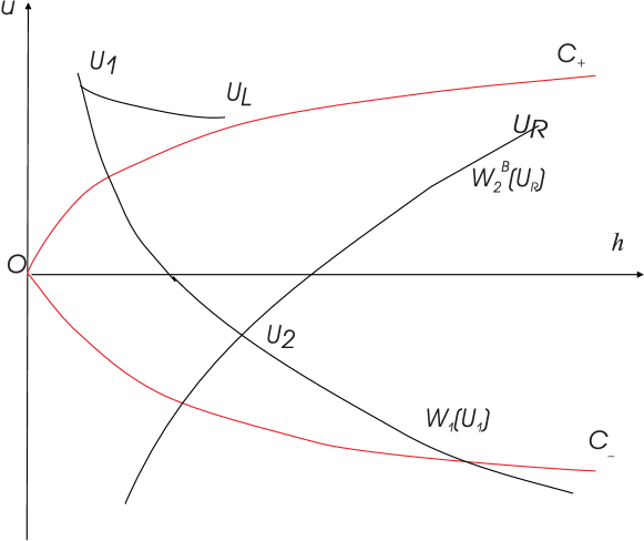
Theorem 4.1.

Let ULA1subscript𝑈𝐿subscript𝐴1U_{L}\in A_{1} and set U1:=SW(UL,aR)assignsubscript𝑈1𝑆𝑊subscript𝑈𝐿subscript𝑎𝑅U_{1}:=SW(U_{L},a_{R}), {U2}=𝒲1(U1)𝒲2B(UR)subscript𝑈2subscript𝒲1subscript𝑈1superscriptsubscript𝒲2𝐵subscript𝑈𝑅\{U_{2}\}=\mathcal{W}_{1}(U_{1})\cap\mathcal{W}_{2}^{B}(U_{R}). Then, the Riemann problem (1.1)-(1.2) admits an admissible solution with the following structure

W3(UL,U1)W1(U1,U2)W2(U2,UR),direct-sumsubscript𝑊3subscript𝑈𝐿subscript𝑈1subscript𝑊1subscript𝑈1subscript𝑈2subscript𝑊2subscript𝑈2subscript𝑈𝑅W_{3}(U_{L},U_{1})\oplus W_{1}(U_{1},U_{2})\oplus W_{2}(U_{2},U_{R}), (4.1)

provided h2h~1subscript2subscript~1h_{2}\leq\tilde{h}_{1}. (Figure 2).

Refer to caption
Figure 2. Solution for ULA1subscript𝑈𝐿subscript𝐴1U_{L}\in A_{1}
Proof.

Observe that the set of composite waves SW(𝒲1(UL),aR)𝑆𝑊subscript𝒲1subscript𝑈𝐿subscript𝑎𝑅SW(\mathcal{W}_{1}(U_{L}),a_{R}) consists of three monotone decreasing curves, and each lies entirely in each region Ai,i=1,2,3formulae-sequencesubscript𝐴𝑖𝑖123A_{i},i=1,2,3. The monotone increasing backward curve 𝒲2B(UR)superscriptsubscript𝒲2𝐵subscript𝑈𝑅\mathcal{W}_{2}^{B}(U_{R}) therefore may cut the three composite curves at a unique point, two point, or else does not meet the wave composite set. The Riemann problem therefore may admit a unique solution, two solutions, or has no solution.

The state ULsubscript𝑈𝐿U_{L} belongs to A1subscript𝐴1A_{1} and in this region, the λ3subscript𝜆3\lambda_{3} is the smallest of the three characteristic speeds. A stationary wave from UL=(hL,uL,aL)subscript𝑈𝐿subscript𝐿subscript𝑢𝐿subscript𝑎𝐿U_{L}=(h_{L},u_{L},a_{L}) to U1=(h1,u1,aR)subscript𝑈1subscript1subscript𝑢1subscript𝑎𝑅U_{1}=(h_{1},u_{1},a_{R}) exists, since aLaRsubscript𝑎𝐿subscript𝑎𝑅a_{L}\leq a_{R}. Moreover, by Lemma 3.6, we have U1A1subscript𝑈1subscript𝐴1U_{1}\in A_{1}.

If h2h1subscript2subscript1h_{2}\leq h_{1}, then the stationary wave is followed by a 111-rarefaction wave with positive speed, and then can be continued by a 222-wave W2(U2,UR)subscript𝑊2subscript𝑈2subscript𝑈𝑅W_{2}(U_{2},U_{R}). If h2>h1subscript2subscript1h_{2}>h_{1}, then the 111-wave in (3.15) is a shock wave. Since h2h¯1subscript2subscript¯1h_{2}\leq\bar{h}_{1} and U1A1subscript𝑈1subscript𝐴1U_{1}\in A_{1}, the shock speed λ2(U1,U2)0subscript𝜆2subscript𝑈1subscript𝑈20\lambda_{2}(U_{1},U_{2})\geq 0, and thus it can follow a stationary wave (with zero speed). Moreover, it is derived from (2.12) that

λ¯1(U1,U2)subscript¯𝜆1subscript𝑈1subscript𝑈2\displaystyle\bar{\lambda}_{1}(U_{1},U_{2}) =u1g2(h2+h22h1),absentsubscript𝑢1𝑔2subscript2superscriptsubscript22subscript1\displaystyle=u_{1}-\sqrt{{g\over 2}\Big{(}h_{2}+{h_{2}^{2}\over h_{1}}\Big{)}},
=h2u2h1u1h2h1absentsubscript2subscript𝑢2subscript1subscript𝑢1subscript2subscript1\displaystyle={h_{2}u_{2}-h_{1}u_{1}\over h_{2}-h_{1}}
=u2g2(h1+h12h2),absentsubscript𝑢2𝑔2subscript1superscriptsubscript12subscript2\displaystyle=u_{2}-\sqrt{{g\over 2}\Big{(}h_{1}+{h_{1}^{2}\over h_{2}}\Big{)}},

thus

λ¯1(U1,U2)subscript¯𝜆1subscript𝑈1subscript𝑈2\displaystyle\bar{\lambda}_{1}(U_{1},U_{2}) u2+g2(hR+hR2h2)=λ¯2(U2,UR).absentsubscript𝑢2𝑔2subscript𝑅superscriptsubscript𝑅2subscript2subscript¯𝜆2subscript𝑈2subscript𝑈𝑅\displaystyle\leq u_{2}+\sqrt{{g\over 2}\Big{(}h_{R}+{h_{R}^{2}\over h_{2}}\Big{)}}=\bar{\lambda}_{2}(U_{2},U_{R}). (4.2)

This means the 111-shock S1(U1,U2)subscript𝑆1subscript𝑈1subscript𝑈2S_{1}(U_{1},U_{2}) can always follow the 222-shock S2(U2,UR)subscript𝑆2subscript𝑈2subscript𝑈𝑅S_{2}(U_{2},U_{R}). Similar for rarefaction waves. Therefore, the solution structure (3.15) holds. \scriptstyle\square

The following theorem deals with the case where the left-hand state ULsubscript𝑈𝐿U_{L} is in A1A2subscript𝐴1subscript𝐴2A_{1}\cup A_{2}.

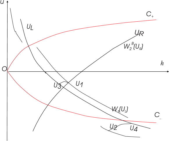
Theorem 4.2.

Let ULA1A2subscript𝑈𝐿subscript𝐴1subscript𝐴2U_{L}\in A_{1}\cup A_{2}. Then there exists a region of values URsubscript𝑈𝑅U_{R} such that SW(𝒲1(UL),aR)𝒲2B(UR)𝑆𝑊subscript𝒲1subscript𝑈𝐿subscript𝑎𝑅superscriptsubscript𝒲2𝐵subscript𝑈𝑅SW(\mathcal{W}_{1}(U_{L}),a_{R})\cap\mathcal{W}_{2}^{B}(U_{R})\neq\emptyset. In this case this intersection may contain either only one or both points U1A2subscript𝑈1subscript𝐴2U_{1}\in A_{2} and U2A3subscript𝑈2subscript𝐴3U_{2}\in A_{3}. The Riemann problem (1.1)-1.2 therefore has a solution with the structure

W1(UL,U3)W3(U3,U1)W2(U1,UR),direct-sumsubscript𝑊1subscript𝑈𝐿subscript𝑈3subscript𝑊3subscript𝑈3subscript𝑈1subscript𝑊2subscript𝑈1subscript𝑈𝑅W_{1}(U_{L},U_{3})\oplus W_{3}(U_{3},U_{1})\oplus W_{2}(U_{1},U_{R}), (4.3)

where U3𝒲1(UL)subscript𝑈3subscript𝒲1subscript𝑈𝐿U_{3}\in\mathcal{W}_{1}(U_{L}) is the point such that U1=SW(U3,aR)subscript𝑈1𝑆𝑊subscript𝑈3subscript𝑎𝑅U_{1}=SW(U_{3},a_{R}), and also

W1(UL,U4)W3(U4,U2)W2(U2,UR),direct-sumsubscript𝑊1subscript𝑈𝐿subscript𝑈4subscript𝑊3subscript𝑈4subscript𝑈2subscript𝑊2subscript𝑈2subscript𝑈𝑅W_{1}(U_{L},U_{4})\oplus W_{3}(U_{4},U_{2})\oplus W_{2}(U_{2},U_{R}), (4.4)

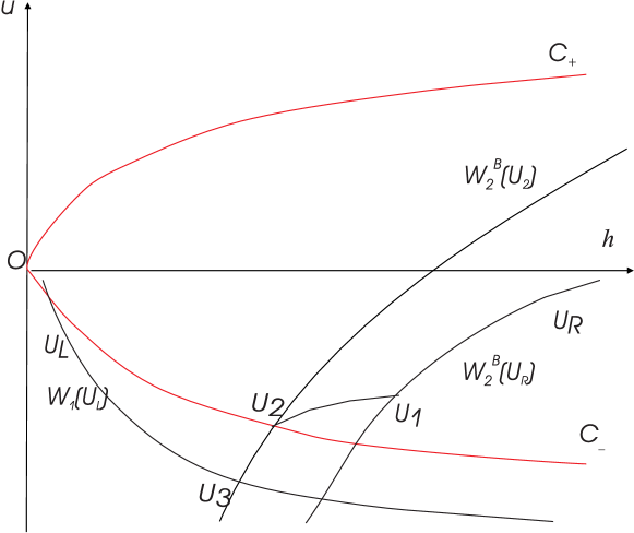
where U4𝒲1(UL)subscript𝑈4subscript𝒲1subscript𝑈𝐿U_{4}\in\mathcal{W}_{1}(U_{L}) is the point such that U2=SW(U4,aR)subscript𝑈2𝑆𝑊subscript𝑈4subscript𝑎𝑅U_{2}=SW(U_{4},a_{R}), if h2h¯Rsubscript2subscript¯𝑅h_{2}\geq\bar{h}_{R} whenever URA2subscript𝑈𝑅superscriptsubscript𝐴2U_{R}\in A_{2}^{-}. (Figure 3 )

Refer to caption
Figure 3. Solution for ULA1A2subscript𝑈𝐿subscript𝐴1subscript𝐴2U_{L}\in A_{1}\cup A_{2}
Proof.

The solution may begin with a 111-wave, either 111-shock with a negative shock speed to a state U3subscript𝑈3U_{3}, or a 111-rarefaction wave with λ1(U3)0subscript𝜆1subscript𝑈30\lambda_{1}(U_{3})\leq 0, followed by a stationary wave W3(U3,U1)subscript𝑊3subscript𝑈3subscript𝑈1W_{3}(U_{3},U_{1}) from U3subscript𝑈3U_{3} to U1subscript𝑈1U_{1}, then followed by a 222-wave W2(U1,UR)subscript𝑊2subscript𝑈1subscript𝑈𝑅W_{2}(U_{1},U_{R}) from U1subscript𝑈1U_{1} to URsubscript𝑈𝑅U_{R}. It is similar in the case of U2subscript𝑈2U_{2}. However, in order that the stationary wave W3(U4,U2)subscript𝑊3subscript𝑈4subscript𝑈2W_{3}(U_{4},U_{2}), for some U4𝒲1(UL)subscript𝑈4subscript𝒲1subscript𝑈𝐿U_{4}\in\mathcal{W}_{1}(U_{L}) and U4A3subscript𝑈4subscript𝐴3U_{4}\in A_{3} obviously, to be followed by a 222-wave W2(U2,UR)subscript𝑊2subscript𝑈2subscript𝑈𝑅W_{2}(U_{2},U_{R}), it is required that the wave is a shock with non-negative shock speed λ2(U2,UR)subscript𝜆2subscript𝑈2subscript𝑈𝑅\lambda_{2}(U_{2},U_{R}). This is equivalent to h2h¯Rsubscript2subscript¯𝑅h_{2}\geq\bar{h}_{R}. \scriptstyle\square

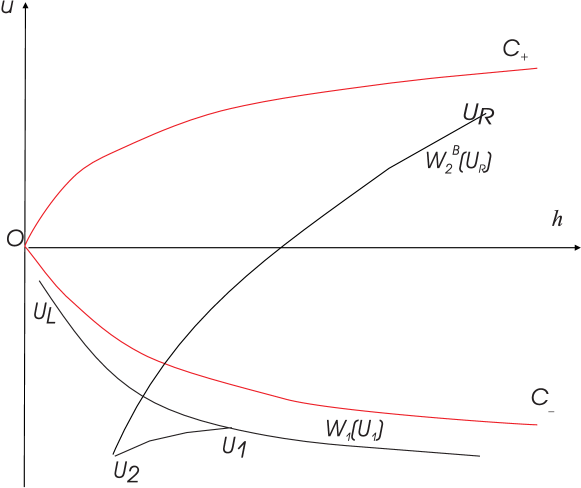
Theorem 4.3.

Let ULA3subscript𝑈𝐿subscript𝐴3U_{L}\in A_{3} and URA1A2subscript𝑈𝑅subscript𝐴1subscript𝐴2U_{R}\in A_{1}\cup A_{2}, and set U1=SW(𝒲2B(UR),aL)𝒲1(UL)subscript𝑈1𝑆𝑊superscriptsubscript𝒲2𝐵subscript𝑈𝑅subscript𝑎𝐿subscript𝒲1subscript𝑈𝐿U_{1}=SW(\mathcal{W}_{2}^{B}(U_{R}),a_{L})\cap\mathcal{W}_{1}(U_{L}) and U2=SW(U1,aR)𝒲2B(UR)subscript𝑈2𝑆𝑊subscript𝑈1subscript𝑎𝑅superscriptsubscript𝒲2𝐵subscript𝑈𝑅U_{2}=SW(U_{1},a_{R})\in\mathcal{W}_{2}^{B}(U_{R}).

  • (i)

    If U1A2+𝒞+{u=0}subscript𝑈1superscriptsubscript𝐴2subscript𝒞𝑢0U_{1}\in A_{2}^{+}\cup\mathcal{C}_{+}\cup\{u=0\}, the Riemann problem (1.1)-(1.2) has a solution with the following structure

    W1(UL,U1)W3(U1,U2)W2(U2,UR).direct-sumsubscript𝑊1subscript𝑈𝐿subscript𝑈1subscript𝑊3subscript𝑈1subscript𝑈2subscript𝑊2subscript𝑈2subscript𝑈𝑅W_{1}(U_{L},U_{1})\oplus W_{3}(U_{1},U_{2})\oplus W_{2}(U_{2},U_{R}). (4.5)
  • (ii)

    If U1A2𝒞subscript𝑈1superscriptsubscript𝐴2subscript𝒞U_{1}\in A_{2}^{-}\cup\mathcal{C}_{-}, provided hRh¯2subscript𝑅subscript¯2h_{R}\geq\bar{h}_{2}, the Riemann solution (4.5) also exists.

  • (iii)

    If U1A1A3subscript𝑈1subscript𝐴1subscript𝐴3U_{1}\in A_{1}\cup A_{3}, the construction (4.5) does not make sense.

(Figure 4).

Refer to caption
Figure 4. Solution for ULA3subscript𝑈𝐿subscript𝐴3U_{L}\in A_{3}
Proof.

If U1A2𝒞subscript𝑈1subscript𝐴2𝒞U_{1}\in A_{2}\cup\mathcal{C}, the non-positive speed wave W1(UL,U1)subscript𝑊1subscript𝑈𝐿subscript𝑈1W_{1}(U_{L},U_{1}) can be followed by a stationary wave W3(U1,U2)subscript𝑊3subscript𝑈1subscript𝑈2W_{3}(U_{1},U_{2}).

When U2A2subscript𝑈2limit-fromsubscript𝐴2U_{2}\in A_{2}-, if U1A2+𝒞+{u=0}subscript𝑈1superscriptsubscript𝐴2subscript𝒞𝑢0U_{1}\in A_{2}^{+}\cup\mathcal{C}_{+}\cup\{u=0\}, then this stationary wave can always be followed by a 222-wave W2(U2,UR)subscript𝑊2subscript𝑈2subscript𝑈𝑅W_{2}(U_{2},U_{R}), since the wave speed of the 222-wave is positive. This establishes (i).

If U1A2𝒞subscript𝑈1superscriptsubscript𝐴2subscript𝒞U_{1}\in A_{2}^{-}\cup\mathcal{C}_{-}, the wave speed of the 222-wave W2(U2,UR)subscript𝑊2subscript𝑈2subscript𝑈𝑅W_{2}(U_{2},U_{R}) is non-negative if and only if hRh¯2subscript𝑅subscript¯2h_{R}\geq\bar{h}_{2}. This proves (ii).

If U1A1subscript𝑈1subscript𝐴1U_{1}\in A_{1}, the 111-wave has positive speed. So it can not be followed by a stationary wave. If U1A3subscript𝑈1subscript𝐴3U_{1}\in A_{3}, then U2A3subscript𝑈2subscript𝐴3U_{2}\in A_{3} by the (MC) criterion. So the 222-wave W2(U2,UR)subscript𝑊2subscript𝑈2subscript𝑈𝑅W_{2}(U_{2},U_{R}) has negative speed. So it can not be proceeded by a stationary wave. This proves (iii). \scriptstyle\square

The above theorem enables URsubscript𝑈𝑅U_{R} to vary in each region A1,A2subscript𝐴1subscript𝐴2A_{1},A_{2}, and A3subscript𝐴3A_{3}. The next theorem enables ULsubscript𝑈𝐿U_{L} to vary in all the three regions.

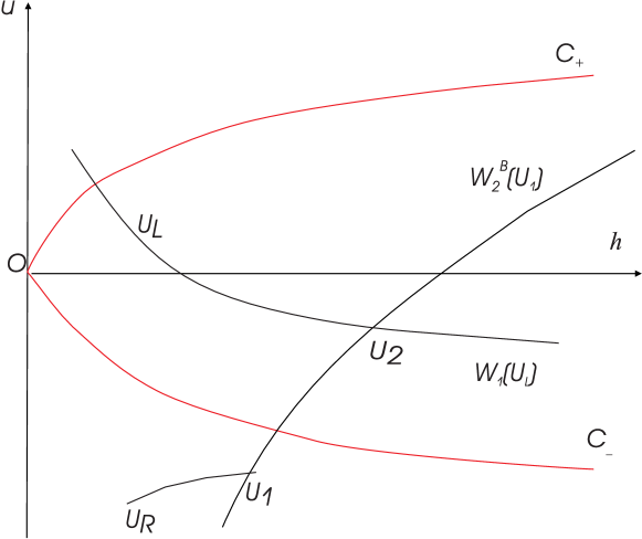
Theorem 4.4.

Let URA3subscript𝑈𝑅subscript𝐴3U_{R}\in A_{3}. Set U1=SW(UR,aL)subscript𝑈1𝑆𝑊subscript𝑈𝑅subscript𝑎𝐿U_{1}=SW(U_{R},a_{L}), U2=𝒲2B(U1)𝒲1(UL)subscript𝑈2superscriptsubscript𝒲2𝐵subscript𝑈1subscript𝒲1subscript𝑈𝐿U_{2}=\mathcal{W}_{2}^{B}(U_{1})\cap\mathcal{W}_{1}(U_{L}). A Riemann solution exists and has the following structure

W1(UL,U2)W2(U2,U1)W3(U1,UR),direct-sumsubscript𝑊1subscript𝑈𝐿subscript𝑈2subscript𝑊2subscript𝑈2subscript𝑈1subscript𝑊3subscript𝑈1subscript𝑈𝑅W_{1}(U_{L},U_{2})\oplus W_{2}(U_{2},U_{1})\oplus W_{3}(U_{1},U_{R}), (4.6)

provided h2h¯1subscript2subscript¯1h_{2}\leq\bar{h}_{1}. (Figure 5).

Refer to caption
Figure 5. ULsubscript𝑈𝐿U_{L} may be anywhere
Proof.

The stationary wave W3(U1,UR)subscript𝑊3subscript𝑈1subscript𝑈𝑅W_{3}(U_{1},U_{R}) turns out to have the greatest wave speed. In order for this wave to be proceeded by the 222-wave W2(U1,U2)subscript𝑊2subscript𝑈1subscript𝑈2W_{2}(U_{1},U_{2}), the wave speed of this 222-wave has to be non-positive. This is equivalent to the condition h2h¯1subscript2subscript¯1h_{2}\leq\bar{h}_{1}, according to Proposition (3.5). Similar to (4.4), we have

λ1(UL,U2)λ2(U2,U1).subscript𝜆1subscript𝑈𝐿subscript𝑈2subscript𝜆2subscript𝑈2subscript𝑈1\lambda_{1}(U_{L},U_{2})\leq\lambda_{2}(U_{2},U_{1}).

so that the 111-wave W1(UL,U2)subscript𝑊1subscript𝑈𝐿subscript𝑈2W_{1}(U_{L},U_{2}) can follow the 222-wave W2(U2,U1)subscript𝑊2subscript𝑈2subscript𝑈1W_{2}(U_{2},U_{1}). \scriptstyle\square

4.2. Solutions containing more than one wave of each characteristic family

It is remarkable feature of the shallow water system that we can also construct solutions with four elementary waves, using three available characteristic fields. This illustrates one of the difficulties in coping with the Riemann problem when the system under consideration is not strictly hyperbolic.

Theorem 4.5.
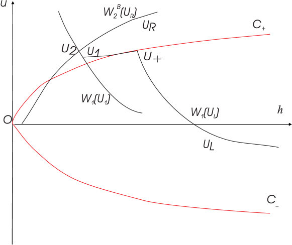
Let ULA2A3subscript𝑈𝐿subscript𝐴2subscript𝐴3U_{L}\in A_{2}\cup A_{3} and set U+=𝒲1(UL)𝒞+,{U1}=SW(U+,aR)A1,{U2}=𝒲1(U1)𝒲2B(UR)formulae-sequencesubscript𝑈subscript𝒲1subscript𝑈𝐿subscript𝒞formulae-sequencesubscript𝑈1𝑆𝑊subscript𝑈subscript𝑎𝑅subscript𝐴1subscript𝑈2subscript𝒲1subscript𝑈1superscriptsubscript𝒲2𝐵subscript𝑈𝑅U_{+}=\mathcal{W}_{1}(U_{L})\cap\mathcal{C}_{+},\{U_{1}\}=SW(U_{+},a_{R})\cap A_{1},\{U_{2}\}=\mathcal{W}_{1}(U_{1})\cap\mathcal{W}_{2}^{B}(U_{R}). The Riemann problem (1.1)-(1.2) has a solution with the following structure

R1(UL,U+)W3(U+,U1)W1(U1,U2)W2(U2,UR),direct-sumsubscript𝑅1subscript𝑈𝐿subscript𝑈subscript𝑊3subscript𝑈subscript𝑈1subscript𝑊1subscript𝑈1subscript𝑈2subscript𝑊2subscript𝑈2subscript𝑈𝑅R_{1}(U_{L},U_{+})\oplus W_{3}(U_{+},U_{1})\oplus W_{1}(U_{1},U_{2})\oplus W_{2}(U_{2},U_{R}), (4.7)

provided h2h~1subscript2subscript~1h_{2}\leq\tilde{h}_{1}. (Figure 6).

Refer to caption
Figure 6. Solution with repeated two 111-waves
Theorem 4.6.

For any ULsubscript𝑈𝐿U_{L}, set {U1}=SW(𝒞,aR)𝒲2B(UR)A2subscript𝑈1𝑆𝑊subscript𝒞subscript𝑎𝑅superscriptsubscript𝒲2𝐵subscript𝑈𝑅subscript𝐴2\{U_{1}\}=SW(\mathcal{C}_{-},a_{R})\cap\mathcal{W}_{2}^{B}(U_{R})\cap A_{2}, U2=(h2,u2,aL)𝒞subscript𝑈2subscript2subscript𝑢2subscript𝑎𝐿subscript𝒞U_{2}=(h_{2},u_{2},a_{L})\in\mathcal{C}_{-} such that U1=SW(U2)subscript𝑈1𝑆𝑊subscript𝑈2U_{1}=SW(U_{2}), and {U3}=𝒲2B(U2)𝒲1(UL).subscript𝑈3superscriptsubscript𝒲2𝐵subscript𝑈2subscript𝒲1subscript𝑈𝐿\{U_{3}\}=\mathcal{W}_{2}^{B}(U_{2})\cap\mathcal{W}_{1}(U_{L}). Then the Riemann problem (1.1)-(1.2) has a solution with the following structure

W1(UL,U3)R2(U3,U2)W3(U2,U1)W2(U1,UR),direct-sumsubscript𝑊1subscript𝑈𝐿subscript𝑈3subscript𝑅2subscript𝑈3subscript𝑈2subscript𝑊3subscript𝑈2subscript𝑈1subscript𝑊2subscript𝑈1subscript𝑈𝑅W_{1}(U_{L},U_{3})\oplus R_{2}(U_{3},U_{2})\oplus W_{3}(U_{2},U_{1})\oplus W_{2}(U_{1},U_{R}), (4.8)

provided hRh¯1subscript𝑅subscript¯1h_{R}\geq\bar{h}_{1} and h3h2subscript3subscript2h_{3}\leq h_{2}. (Figure 7).

Refer to caption
Figure 7. Solution with repeated two 222-waves

Thus, we see that the Riemann problem (1.1)-(1.2) has a solution consisting of a 111-, a 333-, and two 222-waves.

It is interesting to note that there are solutions satisfying the (MC) criterion which contain three waves with the same speed (zero). This is the case when a stationary wave jumps from the level a=aL𝑎subscript𝑎𝐿a=a_{L} to an intermediate level amsubscript𝑎𝑚a_{m} between aLsubscript𝑎𝐿a_{L} and aRsubscript𝑎𝑅a_{R}, followed by an ”intermediate” k𝑘k-shock with zero speed at the level amsubscript𝑎𝑚a_{m}, k=1,3𝑘13k=1,3, and then followed by another stationary wave jumping from the level amsubscript𝑎𝑚a_{m} to aRsubscript𝑎𝑅a_{R}. Thus, there are only two possibilities:

  • (i)

    ULsubscript𝑈𝐿U_{L} belongs to A1subscript𝐴1A_{1} and a 111-shock with zero speed is used.

  • (ii)

    URsubscript𝑈𝑅U_{R} belongs to A3subscript𝐴3A_{3} and a 222-shock with zero speed is used.

We just describe the first case (i), as the second case is similar. Recall from Proposition 3.5 that for any UA1𝑈subscript𝐴1U\in A_{1}, there exists a unique point denoted by U~𝒲1(U)A2~𝑈subscript𝒲1𝑈subscript𝐴2\tilde{U}\in\mathcal{W}_{1}(U)\cap A_{2} such that

λ¯1(U,U~)=0.subscript¯𝜆1𝑈~𝑈0\bar{\lambda}_{1}(U,\tilde{U})=0.
Theorem 4.7.

Let ULA1subscript𝑈𝐿subscript𝐴1U_{L}\in A_{1} and set

SW(UL,[aL,aR]):=a[aL,aR]SW(UL,a),assign𝑆𝑊subscript𝑈𝐿subscript𝑎𝐿subscript𝑎𝑅subscript𝑎subscript𝑎𝐿subscript𝑎𝑅𝑆𝑊subscript𝑈𝐿𝑎\displaystyle SW(U_{L},[a_{L},a_{R}]):=\cup_{a\in[a_{L},a_{R}]}SW(U_{L},a),
SW~(UL,[aL,aR]):={U~|USW(UL,[aL,aR])}.assign~𝑆𝑊subscript𝑈𝐿subscript𝑎𝐿subscript𝑎𝑅conditional-set~𝑈𝑈𝑆𝑊subscript𝑈𝐿subscript𝑎𝐿subscript𝑎𝑅\displaystyle\widetilde{SW}(U_{L},[a_{L},a_{R}]):=\{\tilde{U}|\ U\in SW(U_{L},[a_{L},a_{R}])\}.

Whenever

SW~(UL,[aL,aR])𝒲2B(UR)~𝑆𝑊subscript𝑈𝐿subscript𝑎𝐿subscript𝑎𝑅superscriptsubscript𝒲2𝐵subscript𝑈𝑅\widetilde{SW}(U_{L},[a_{L},a_{R}])\cap\mathcal{W}_{2}^{B}(U_{R})\neq\emptyset

there exist am[aL,aR]subscript𝑎𝑚subscript𝑎𝐿subscript𝑎𝑅a_{m}\in[a_{L},a_{R}], U1=SW(UL,am)subscript𝑈1𝑆𝑊subscript𝑈𝐿subscript𝑎𝑚U_{1}=SW(U_{L},a_{m}), and

U2SW~(UL,[aL,aR])𝒲2B(UR)subscript𝑈2~𝑆𝑊subscript𝑈𝐿subscript𝑎𝐿subscript𝑎𝑅superscriptsubscript𝒲2𝐵subscript𝑈𝑅U_{2}\in\widetilde{SW}(U_{L},[a_{L},a_{R}])\cap\mathcal{W}_{2}^{B}(U_{R})

that defines a solution with the structure

W3(UL,U1)S1(U1,U~1)W3(U~1,U2)W2(U2,UR).direct-sumsubscript𝑊3subscript𝑈𝐿subscript𝑈1subscript𝑆1subscript𝑈1subscript~𝑈1subscript𝑊3subscript~𝑈1subscript𝑈2subscript𝑊2subscript𝑈2subscript𝑈𝑅W_{3}(U_{L},U_{1})\oplus S_{1}(U_{1},\tilde{U}_{1})\oplus W_{3}(\tilde{U}_{1},U_{2})\oplus W_{2}(U_{2},U_{R}). (4.9)

Acknowledgments

The first author (P.G.L.) was supported by the A.N.R. Grant 06-2-134423: Mathematical methods in general relativity (MATH-GR) and the Centre National de la Recherche Scientifique (CNRS).

References

  • [1] A. Alcrudo and F. Benkhaldoun, Exact solutions to the Riemann problem of the shallow water equations with a bottom step, Computers & Fluids 30 (2001), 643–671.
  • [2] D. Amadori, L. Gosse, and G. Guerra, Godunov-type approximation for a general resonant balance law with large data, J. Differential Equations 198 (2004), 233–274.
  • [3] N. Andrianov and G. Warnecke, On the solution to the Riemann problem for the compressible duct flow. SIAM J. Appl. Math., 64(3):878 901, 2004.
  • [4] E. Audusse, F. Bouchut, M-O. Bristeau, R. Klein, and B. Perthame, A fast and stable well-balanced scheme with hydrostatic reconstruction for shallow water flows. SIAM J. Sci. Comp., 25(6):2050–2065, 2004.
  • [5] F. Bouchut, Nonlinear stability of finite volume methods for hyperbolic conservation laws and well-balanced schemes for sources, Frontiers in Mathematics. Birkhäuser Verlag, Bäsel, 2004.
  • [6] M.J. Castro, J.A. Garc a-Rodr guez, J.M. Gonz lez-Vida, and C. Par s, A parallel 2D finite volume scheme for solving the bilayer shallow-water system: modellization of water exchange at the Strait of Gibraltar, Parallel computational fluid dynamics, 199–206, Elsevier B. V., Amsterdam, 2005.
  • [7] G. Dal Maso, P.G. LeFloch, and F. Murat, Definition and weak stability of nonconservative products. J. Math. Pures Appl., 74:483–548, 1995.
  • [8] P. Goatin and P.G. LeFloch, The Riemann problem for a class of resonant nonlinear systems of balance laws. Ann. Inst. H. Poincaré Anal. Nonlinéaire, 21:881–902, 2004.
  • [9] L. Gosse, Localization effects and measure source terms in numerical schemes for balance laws, Math. Comp. 71 (2002), 553–582.
  • [10] L. Gosse and G. Toscani, Asymptotic-preserving and well-balanced schemes for radiative transfer and the Rosseland approximation, Numer. Math. 98 (2004), no. 2, 223–250.
  • [11] J.M. Greenberg, A.Y. Leroux, R. Baraille, and A. Noussair, Analysis and approximation of conservation laws with source terms. SIAM J. Numer. Anal., 34:1980–2007, 1997.
  • [12] B.T. Hayes and P.G. LeFloch, Nonclassical shock waves and kinetic relations: Strictly hyperbolic systems, SIAM J. Math. Anal. 31 (2000), 941–991.
  • [13] T.Y. Hou and P.G. LeFloch, Why nonconservative schemes converge to wrong solutions: error analysis, Math. Comp. 62 (1994), 497–530.
  • [14] E. Isaacson and B. Temple, Nonlinear resonance in systems of conservation laws. SIAM J. Appl. Math., 52:1260–1278, 1992.
  • [15] E. Isaacson and B. Temple, Convergence of the 2×2222\times 2 godunov method for a general resonant nonlinear balance law. SIAM J. Appl. Math., 55:625–640, 1995.
  • [16] D. Kröner and M.D. Thanh, Numerical solutions to compressible flows in a nozzle with variable cross-section. SIAM J. Numer. Anal., 43(2):796–824, 2005.
  • [17] P.D. Lax, Shock waves and entropy, in: E.H. Zarantonello, Ed.,. Contributions to Nonlinear Functional Analysis, pp. 603–634, 1971.
  • [18] P.G. LeFloch, Shock waves for nonlinear hyperbolic systems in nonconservative form. Institute for Math. and its Appl., Minneapolis, Preprint, 593, 1989.
  • [19] P.G. LeFloch, Hyperbolic Systems of Conservation Laws: The theory of classical and nonclassical shock waves, Lectures in Mathematics, ETH Zuerich, Birkhauser, 2002.
  • [20] P.G. LeFloch, Graph solutions of nonlinear hyperbolic systems, J. Hyper. Diff. Equa. 1:243–289, 2004.
  • [21] P.G. LeFloch and M.D. Thanh, The Riemann problem for fluid flows in a nozzle with discontinuous cross-section. Comm. Math. Sci., 1(4):763–797, 2003.
  • [22] D. Marchesin and P.J. Paes-Leme, A Riemann problem in gas dynamics with bifurcation. Hyperbolic partial differential equations III. Comput. Math. Appl. (Part A), 12:433–455, 1986.