Event-by-event simulation of Einstein-Podolsky-Rosen-Bohm experiments

Abstract

We construct an event-based computer simulation model of the Einstein-Podolsky-Rosen-Bohm experiments with photons. The algorithm is a one-to-one copy of the data gathering and analysis procedures used in real laboratory experiments. We consider two types of experiments, those with a source emitting photons with opposite but otherwise unpredictable polarization and those with a source emitting photons with fixed polarization. In the simulation, the choice of the direction of polarization measurement for each detection event is arbitrary. We use three different procedures to identify pairs of photons and compute the frequency of coincidences by analyzing experimental data and simulation data. The model strictly satisfies Einstein’s criteria of local causality, does not rely on any concept of quantum theory and reproduces the results of quantum theory for both types of experiments. We give a rigorous proof that the probabilistic description of the simulation model yields the quantum theoretical expressions for the single- and two-particle expectation values.

I Introduction

A fundamental problem, originating from the work of Einstein, Podolsky and Rosen (EPR) Einstein et al. (1935) and reformulated by Bohm Bohm (1951) is to explain how individual detection events, registered by different detectors in such a way that a measurement on one particle does not have a causal effect on the result of the measurement on another particle (Einstein’s criterion of local causality), give rise to the two-particle quantum correlations that are found in experiments Freedman and Clauser (1972); Aspect et al. (1982a, b); Tapster et al. (1994); Tittel et al. (1998); Weihs et al. (1998); Weihs (2000); Rowe et al. (2001); Fatal et al. (2004); Sakai et al. (2006).

In Einstein-Podolsky-Rosen-Bohm (EPRB) experiments, individual events are registered, correlations between them are calculated and are found to correspond to the two-particle correlation for the singlet state. Since, in quantum theory, the basic equation that describes individual events is not known Home (1997), quantum theory simply cannot be used to construct a numerical algorithm to simulate the individual events. Of course, using pseudo-random numbers we could generate events according to the probability distribution that is obtained by solving the Schrödinger equation. However, the challenge is to explain how the individual events can give rise to the two-particle correlations of the singlet state without invoking concepts of quantum theory.

The question that we address in this paper is: Given the existing experimental data (numbers recorded during an experiment, stored on computer disks, and analyzed long after the data is taken), that, when analyzed properly, yields expectation values which are in good agreement with the predictions of quantum theory Freedman and Clauser (1972); Aspect et al. (1982b); Tapster et al. (1994); Tittel et al. (1998); Weihs et al. (1998); Sakai et al. (2006), is it possible to construct an event-based simulation algorithm that satisfies Einstein’s criteria of local causality, generates the same kind of data as in experiment, and is capable of reproducing exactly the single- and two-particle averages of quantum theory for a system of two $S=1/2$ particles?

Within the context of local realist probabilistic models, a rigorous proof that the existence of an algorithm that describes the outcome of real EPRB experiments cannot be excluded, has been given earlier Larsson and Gill (2004). Although such a proof is very valuable, actually finding such algorithms using local, causal processes to generate the probability distributions of quantum theory, is another challenge.

In this paper, we present results of a complete simulation of Aspect-type experiments using an Einstein local, causal event-based simulation model. An important feature in these experiments is the arbitrariness in the choice of the directions in which the polarization will be measured, for each individual detection event Freedman and Clauser (1972); Aspect et al. (1982a, b); Tapster et al. (1994); Tittel et al. (1998); Weihs et al. (1998). This feature has not been taken into account in our earlier work De Raedt et al. (2006) but is fully accounted for in the simulation procedure that we describe in this paper.

The paper is organized as follows. In Section II we describe the experimental set-up, the data gathering method and the data analysis procedures used in EPRB experiments with photons, closely following Ref. Weihs et al. (1998); Aspect et al. (1982b). The sources used in EPRB experiments emit photons with opposite but otherwise unpredictable polarization. Each photon propagates to an observation station consisting of a polarizer and two detectors. In accordance with quantum theory and experiments, we expect the two-particle correlation to agree with the expression obtained by assuming that the quantum state is a singlet. We refer to this experimental set-up as Case I. Inserting polarizers between the source and the observation stations changes the pair generation procedure such that the two photons that enter the observation stations have a fixed polarization. In this case, the photon intensity recorded by the detectors behind the polarizers in each observation station obeys Malus law. We refer to this set-up as Case II. A brief review of the quantum theoretical description of Cases I and II is given in Section III.

In real experiments, macroscopic or microscopic, we need a well-defined procedure to decide if two detection events stem from a single system. In real EPRB experiments with photons, the time at which the events are registered is used for this purpose. However, the criterion that is used to select the events that stem from a single two-particle system is, to considerable extent, arbitrary. In Section IV, we study this aspect by analyzing publicly available experimental data for an EPRB experiment with photons Weihs et al. (1998). We present results of an analysis using three different procedures:

• First, we simply divide the time interval of measurement in equally spaced bins GIL . For each station, we determine the number of events per bin. From this data, we compute the coincidences. Effectively, this procedure compares the detection times at both stations with the time of a reference clock, using a coincidence window with a width that is equal to the bin size.

• Second, we employ the criterion used in the experiment Weihs et al. (1998); Weihs (2000). We compute the coincidences of a detection event at station 1 and a detection event at station 2 by comparing the time difference of these events with a fixed time window, that is we use relative times to determine the coincidences.

• Finally, in the third procedure Weihs (2000), we first maximize the number of coincidences by shifting by the same amount, the detection times of station 2 relative to those of station 1, and then use the second procedure to count the coincidences. This two-step procedure reproduces the published results Weihs et al. (1998).

Our analysis shows that the first and third procedure may yield a result that is in reasonable agreement with the prediction of quantum theory if the bin size or coincidence window is sufficiently small. The data obtained by the second procedure is similar except that for a particular choice of the time window, the result is in conflict with quantum theory. In general, these results support the idea that the idealized EPRB gedanken experiment Bell (1993); Santos (2005); Ẑukowksi (2005) that agrees with quantum theory cannot be performed Gill (2003).

In Section V we describe an Einstein local, causal event-based computer simulation model, based on the EPRB experiment with photons performed by Weihs et al Weihs et al. (1998); Weihs (2000). The crucial point of the present and of our earlier work De Raedt et al. (2006, 2007a, 2007b, 2007c) is that we simulate a model of the real EPRB experiments, not of the simplified, gedanken-type version that is commonly used Bell (1993); Santos (2005); Ẑukowksi (2005). We give an explicit description of the algorithm to simulate the photons one by one, the observation stations containing the polarizers and detectors, and the data analysis procedure. The polarizers are modeled such that we reproduce the quantum theoretical results for Case I and Case II without changing the algorithm for the polarizers, that is the functionality of all polarizers is the same. In contrast to the real EPRB experiments with photons Weihs et al. (1998); Weihs (2000), the number of orientations per polarizer to choose from is not limited to two.

Section VI gives a rigorous analytical treatment of the probabilistic model of our simulation algorithm and proves that this model can reproduce the single-particle averages and the two-particle correlation of a system of two quantum spins for Cases I and II. This probabilistic model is identical to the one studied in Ref. Larsson and Gill (2004), except for the concrete model of the time-delay mechanism. In Section VII we present our simulation data and demonstrate that there is excellent agreement with the results obtained from quantum theory and the probabilistic model. In Section VIII, we study the effect of the time window on the frequency of coincidences and show that the simulation model readily reproduces published experimental data, including the statististics of the single-detection events. A summary of our results is given in Section IX.

Figure 1: (color online) Case I: Schematic diagram of an EPRB experiment with randomly polarized particles.

Figure 2: (color online) Case II: Schematic diagram of an EPRB experiment with particles with fixed polarization.

II EPRB experiment with photons

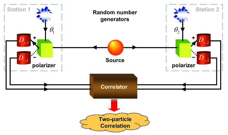
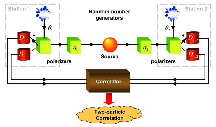
A schematic diagram of Case I is shown in Fig. 1. A source emits pairs of photons with opposite but otherwise unpredictable polarization. Each photon of a pair propagates to an observation station in which it is manipulated and detected. The two stations are separated spatially and temporally. This arrangement prevents the observation at station 1 (2) to have a causal effect on the data registered at station $2$ (1). In Case II (see Fig. 2), additional polarizers are inserted between the source and the observation stations Aspect et al. (1982b) such that the two photons that enter the observation stations have a fixed polarization. We denote the orientations of these polarizers by the angles $\eta_{1}$ and $\eta_{2}$.

As the photon arrives at station $i=1,2$, it passes through a polarizer. The orientation of the polarizer in observation station $i$ is characterized by the angle $\theta_{i}$, which may be chosen at random. As the photon leaves the polarizer, it generates a signal in one of the two detectors. Each station has its own clock (not shown) that assigns a time-tag to each signal generated by one of the two detectors Weihs et al. (1998); Weihs (2000). Effectively, this procedure discretizes time in intervals, the width of which is determined by the time-tag resolution $\tau$. In experiment, the time-tag generators are synchronized before each run Weihs et al. (1998); Weihs (2000). This procedure is necessary because in time, the clocks may become unsynchronized Weihs et al. (1998); Weihs (2000).

Note that the description given earlier is only a pictorial description of real EPRB experiments with photons, as they are carried out in a laboratory. The experimental facts are the settings of the various apparatuses and the detection events. What happens in between activating the source and the registration of the detection events is not, or cannot be, measured and is therefore not known. In this sense, the photon should be regarded as an element of a model or theory for the real laboratory experiment only.

In the experiment, the firing of a detector is regarded as an event. At the $n$th event, the data recorded on a hard disk (not shown) at station $i=1,2$ consists of $\theta_{n,i}$, $x_{n,i}=\pm 1$, specifying which of the two detectors behind the selected polarizer fired and the time tag $t_{n,i}$ indicating the time at which a detector fired. Hence, the set of data collected at station $i=1,2$ during a run of $N$ events may be written as

$$\Upsilon_{i}=\left\{{x_{n,i},t_{n,i},\theta_{n,i}|n=1,\ldots,N}\right\}.$$ (1)

Any real EPRB experiment requires some criterion to decide which detection events are to be considered as stemming from a single two-particle system. In EPRB-type experiments with photons, this decision is taken on the basis of coincidence in time Weihs et al. (1998); Clauser and Horne (1974). However, as discussed in Section IV, this identification procedure is not unique. Coincidences can, for example, be identified by comparing the time differences $\{t_{n,1}-t_{n,2}|n=1,\ldots,N\}$ with a window $W$ Weihs et al. (1998). In this case, for each pair of rotation angles $\alpha$ and $\beta$, the number of coincidences between detectors $D_{x,1}$ ($x=\pm$1) at station 1 and detectors $D_{y,2}$ ($y=\pm$1) at station 2 is given by

$$C_{xy}=C_{xy}(\alpha,\beta)= \sum_{n=1}^{N} \delta_{x,x_{n,1}}\delta_{y,x_{n,2}}\delta_{\alpha,\theta_{n,1}}\delta_{\beta,\theta_{n,2}}$$ (2)

$$\times\Theta(W-|t_{n,1}-t_{n,2}|),$$

where $\Theta(t)$ is the Heaviside step function. The single-particle averages and correlation between the coincidence counts are then given by

$$E_{1}(\alpha,\beta) = \frac{\sum_{x,y=\pm 1}xC_{xy}}{\sum_{x,y=\pm 1}C_{xy}},$$

$$E_{2}(\alpha,\beta) = \frac{\sum_{x,y=\pm 1}yC_{xy}}{\sum_{x,y=\pm 1}C_{xy}},$$

$$E(\alpha,\beta) = \frac{\sum_{x,y=\pm 1}xyC_{xy}}{\sum_{x,y=\pm 1}C_{xy}}$$ (3)

$$= \frac{C_{++}+C_{--}-C_{+-}-C_{-+}}{C_{++}+C_{--}+C_{+-}+C_{-+}},$$

where the denominators in Eq.(II) are the sum of all coincidences. In practice, the data $\{\Upsilon_{1},\Upsilon_{2}\}$ are analyzed long after the data have been collected Weihs et al. (1998). In general, the values for the coincidences $C_{xy}(\alpha,\beta)$ depend on the time-tag resolution $\tau$ and the window $W$ used to identify the coincidences, independent of which of the three pair identification procedures (see Section IV) is being used.

Data of EPRB experiments are often analyzed in terms of the function Weihs et al. (1998); Clauser et al. (1969)

$$S(\alpha,{\alpha}^{\prime},\beta,{\beta}^{\prime})={E(\alpha,\beta)-E(\alpha,{\beta}^{\prime})}+{E({\alpha}^{\prime},\beta)+E({\alpha}^{\prime},{\beta}^{\prime})},$$ (4)

because it provides clear evidence that a quantum system is described by an entangled state. The idea behind this is that for any product state in quantum theory, or for the class of local realistic theories considered by Bell Bell (1993)

$$-2\leq S(\alpha,\alpha^{\prime},\beta,\beta^{\prime})\leq 2,$$ (5)

an inequality known as one of Bell’s generalized inequalities Clauser et al. (1969). For later use, it is expedient to introduce the function

$$S(\theta)\equiv S(\alpha,\alpha+2\theta,\alpha+\theta,\alpha+3\theta),$$ (6)

where we have fixed the relation between the angles $\beta=\alpha+\theta$, ${\alpha}^{\prime}=\alpha+2\theta$, ${\beta}^{\prime}=\alpha+3\theta$ through the angle $\theta$. Assuming rotational invariance, $S(\theta)$ does not depend on $\alpha$ and we may set $\alpha=0$.

III Quantum Theory

In this section, we give a brief account of the quantum theoretical description of Cases I and II, strictly staying within the axiomatic framework that quantum theory provides.

In the quantum theoretical description of Case I, the whole system is assumed to be described by the two-particle state

$$|\Psi\rangle = \frac{1}{\sqrt{2}}\left({|H\rangle_{1}|V\rangle_{2}-|V\rangle_{1}|H\rangle_{2}}\right)$$ (7)

$$= \frac{1}{\sqrt{2}}\left({|{HV}\rangle-|{VH}\rangle}\right),$$

where $H$ and $V$ denote the horizontal and vertical polarization and the subscripts refer to photon 1 and 2, respectively. The singlet state $|\Psi\rangle$ cannot be written as a product of single-photon states, hence it is an entangled state.

In Case II, the photons have a definite polarization when they enter the observation station and the system is described by the product state

$$|\Psi\rangle=(\cos\eta_{1}|H\rangle_{1}+\sin\eta_{1}|V\rangle_{1})(\cos\eta_{2}|H\rangle_{2}+\sin\eta_{2}|V\rangle_{2}).$$ (8)

The quantum theoretical expectation $P_{+}(\alpha)$ ($P_{-}(\beta)$) for observing a photon at the $+$ ($-$) detector behind the polarizer with orientation $\alpha$ ($\beta$) is given in the first two rows of Table 1. The expressions for the two-particle correlation $E(\alpha,\beta)$ are given in the third row. From Table 1, it is clear that measuring $E_{1}(\alpha)=P_{+}(\alpha)-P_{-}(\alpha)$, $E_{2}(\beta)=P_{+}(\beta)-P_{-}(\beta)$ and $E(\alpha,\beta)$ for various $\alpha$ and $\beta$ suffices to distinguish between systems in the entangled state (Case I) or in the product state (Case II).

Table 1: The single- and two-particle expectation values for the two experiments described by the states Eqs. (7) and (8), respectively.

	Case I	Case II
$P_{+}(\alpha)$	$1/2$	$\cos^{2}(\alpha-\eta_{1})$
$P_{-}(\beta)$	$1/2$	$\sin^{2}(\beta-\eta_{2})$
$E_{1}(\alpha)$	$0$	$\cos 2(\alpha-\eta_{1})$
$E_{2}(\beta)$	$0$	$\cos 2(\beta-\eta_{2})$
$E(\alpha,\beta)$	$-\cos 2(\alpha-\beta)$	$\cos 2(\alpha-\eta_{1})\cos 2(\beta-\eta_{2})$

In Case I, $E(\alpha,\beta)=-\cos 2(\alpha-\beta)$ and we find

$$S(\theta)=3\cos 2\theta-\cos 6\theta,$$ (9)

which reaches its maximum value $S_{max}=\max_{\theta}S(\theta)=2\sqrt{2}$ at $\theta=\pi/8+j\pi/2$, where $j$ is an integer number.

Analysis of the experimental data Freedman and Clauser (1972); Aspect et al. (1982b, a); Tapster et al. (1994); Tittel et al. (1998); Weihs et al. (1998); Rowe et al. (2001); Fatal et al. (2004); Sakai et al. (2006), yields results that are in good agreement with the expressions in Table 1, leading to the conclusion that in a quantum theoretical description of Case I, the state does not factorize, in spite of the fact that the photons are spatially and temporally separated and do not interact.

IV Data analysis of a real EPRB experiment with photons

Figure 3: (color online) Left: $S_{max}$ as a function of the time window $W$, computed from the data sets contained in the archives Alice.zip and Bob.zip that can be downloaded from Ref. WEI . Squares (black): Data obtained by comparing the detection times $\{t_{n,1}|n=1,\ldots,N_{1}=388455\}$ and $\{t_{m,2}|m=1,\ldots,N_{2}=302271\}$ with a reference clock. The maximum value of $S_{max}\approx 2.78$ is found at $W=4$ ns at which the total number of coincidences is 2010 ($\approx 0.6\%$). Crosses (blue): Results of comparing the difference of the detection times with the time window $W$ ($\Delta=0$). The maximum value of $S_{max}\approx 2.89$ is found at $W=3$ ns at which the total number of coincidences (with double counts removed) is 2899 ($\approx 0.8\%$). Bullets (red): Results of comparing the difference of the detection times with the time window $W$, taking into account the time shift $\Delta=4$ ns that maximizes the total number of coincidences, which (with double counts removed) is 13975 ($\approx 4\%$) in this case. The maximum value of $S_{max}\approx 2.73$ is found at $W=2$ ns. Dashed line at $2\sqrt{2}\approx 2.82$: $S_{max}$ if the system is described by quantum theory (see Section III). Dashed line at $2$: $S_{max}$ if the system is described by the class of models introduced by Bell Bell (1993). Right: Same as left except for the range of $W$.

Figure 4: (color online) Frequency of coincidences defined by $2(C_{++}+C_{--}+C_{+-}+C_{-+})/(N_{1}+N_{2})$, as a function of the time window $W$ (bin size $B=2W$). The results were obtained by averaging the data of the four experiments ($\theta_{1}=0,\theta_{2}=\pi/8$), ($\theta_{1}=0,\theta_{2}=3\pi/8$), ($\theta_{1}=\pi/4,\theta_{2}=\pi/8$), and ($\theta_{1}=\pi/4,\theta_{2}=3\pi/8$), contained in the archives Alice.zip and Bob.zip WEI . Squares (black): Data obtained by comparing the detection times $\{t_{n,1}|n=1,\ldots,N_{1}=388455\}$ and $\{t_{m,2}|m=1,\ldots,N_{2}=302271\}$ with a reference clock. Crosses (blue): Results of comparing the difference of the detection times with the time window $W$ ($\Delta=0$). Bullets (red): Results of comparing the difference of the detection times with the time window $W$, taking into account the time shift $\Delta=4$ ns that maximizes the number of coincidences. For the values of $W$ at which the three $S_{max}$ reach their maximum (squares: $W=4$ ns, $S_{max}\approx 2.78$; crosses: $W=3$ ns, $S_{max}\approx 2.89$; bullets: $W=2$ ns, $S_{max}\approx 2.73$), the frequencies of coincidences are approximately $0.0015$, $0.002$, and $0.01$, respectively.

We analyze a data set (the archives Alice.zip and Bob.zip) of a real EPRB experiment with photons that is publicly available WEI . The archives Alice.zip and Bob.zip contain data Eq. (1) for Case I for $\theta_{1}=0,\pi/4$ and $\theta_{2}=\pi/8,3\pi/8$. In a real experiment, such as the one described in Ref. Weihs et al. (1998), the number of events detected at station 1 is unlikely to be the same as the number of events detected at station 2. The data sets of Ref. WEI show that station 1 (Alice.zip) recorded $N_{1}=388455$ events while station 2 (Bob.zip) recorded $N_{2}=302271$ events. The fact that $N_{1}\not=N_{2}$ may have various reasons: It may happen that the source emitted one instead of two photons, one of the detectors did not respond to the arrival of a photon, the detector fired when there was no photon, etc. The data analysis does not account for such possibilities: We use the data as it is, without making additional hypotheses about unknown processes.

We need a well-defined procedure to decide which two detection events stem from two particles that form a pair. Here, we use three different procedures to determine these pairs. Once the coincidences have been identified, we compute the two-particle average and $S_{max}=\max_{\theta}S(\theta)$ using Eqs.(II), (4) and (6), respectively. In addition, we compute the frequency of coincidences, defined by $2(C_{++}+C_{--}+C_{+-}+C_{-+})/(N_{1}+N_{2})$.

The first procedure divides the time interval of measurement (about 10 s) in equally spaced bins of size $B$ GIL . For each station, we use the data $\{t_{n,1}|n=1,\ldots,N_{1}\}$ and $\{t_{m,2}|m=1,\ldots,N_{2}\}$ to determine the number of events per bin and compute the coincidences by examining the content of the bins. This procedure compares the detection times $t_{n,1}$ and $t_{m,2}$ with a reference clock, using a coincidence window $W=B/2$. In the second procedure, we count the coincidences according to Eq. (2). In the third procedure, we account for the fact that in the real EPRB experiment Weihs (2000), there may be an unknown shift $\Delta$ (assumed to be constant during the experiment) between the times $t_{n,1}$ gathered at station 1 and the times $t_{m,2}$ recorded at station 2. Therefore, there is some extra ambiguity in matching the data of station 1 to the data of station 2. A simple data processing procedure that resolves this ambiguity consists of two steps Weihs (2000). First, we make a histogram of the time differences $t_{n,1}-t_{m,2}$ with a small but reasonable time resolution (we used $0.5$ ns). Then, we fix the value of the time-shift $\Delta$ by searching for the time difference for which the histogram reaches its maximum. Thus, we maximize the number of coincidences by a suitable choice of $\Delta$. For the case at hand, we find $\Delta=4$ ns.

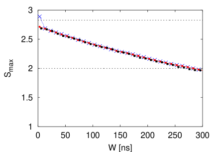
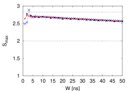
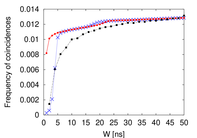
The results for $S_{max}$ and the frequency of coincidences, as obtained by applying the three data analysis procedures, are presented in Figs. 3 and 4, respectively. Note that in general, the frequency of coincidences depends on $\alpha$ and $\beta$. However, for the choice $\alpha=\theta_{1}=0,\pi/4$ and $\beta=\theta_{2}=\pi/8,3\pi/8$, made in experiment Weihs et al. (1998), by symmetry the four relevant frequencies of coincidences are expected to be the same, hence we show their average. As it is clear from Eq. (2) that the width of the time window in the second and third procedure is $2W$, we have taken $B=2W$ to facilitate the comparison.

From Fig. 3, it follows that all three procedures yield a value of $S_{max}$ that significantly exceeds the upperbound ($S_{max}=2$) of the original Bell-like models Bell (1993). As it has been shown rigorously that the original Bell (CHSH) inequality has to be modified if one uses Eq. (2) to count coincidences Larsson and Gill (2004), this violation should not come as a surprise. For $W>10$ ns and disregarding small fluctuations, the general trend is clear: $S_{max}$ decreases with $W$ and drops below the “Bell-bound” for $W>300$ ns. For $W\leq 10$ ns, each of the three procedures yields results for $S_{max}$ that are close to the quantum theoretical upperbound $2\sqrt{2}\approx 2.83$ Cirel’son (1980).

The procedure that maximizes the coincidence count by varying $\Delta$ reduces the maximum value of $S_{max}$ from a value 2.89 ($\Delta=0$) that considerably exceeds the maximum ($2\sqrt{2}$) for the quantum system Cirel’son (1980) to a value 2.73 (the value cited in Ref. Weihs et al. (1998)) that violates the Bell inequality Bell (1993) and is less than the maximum for the quantum system. The fact that the “uncorrected” data ($\Delta=0$) violate the rigorous bound for the quantum system should not be taken as evidence that quantum theory is “wrong”: It merely indicates that the way in which the data of the two stations has been grouped in two-particle events is not optimal.

Analyzing the experimental data set WEI with $\Delta=4$ns and $W=2$ns (yielding the “best” value of $S_{max}\approx 2.73$ and a total number of coincidences of 13975) gives $E_{1}(0,\pi/8)=-0.073$, $E_{1}(0,3\pi/8)=0.118$, $E_{1}(\pi/4,\pi/8)=0.036$, $E_{1}(\pi/4,3\pi/8)=-0.065$, and $E_{2}(0,\pi/8)=0.188$, $E_{2}(0,3\pi/8)=0.258$, $E_{2}(\pi/4,\pi/8)=0.099$, $E_{2}(\pi/4,3\pi/8)=-0.147$, significantly different from the theoretically expected value (zero, see Table 1). Disregarding the coincidence criterion, we find $\sum_{n}x_{n,1}=-0.007,-0.005$ for $\alpha=0,\pi/4$ and $\sum_{n}x_{n,2}=-0.028,-0.024$ for $\beta=\pi/8,3\pi/4$. Apparently, all these numbers change considerably with the station and with the settings of the electro-optic modulators.

The results presented in Fig. 4, show that for small $W$, the frequency of coincidences depends significantly on the criterion that is used to identify pairs of events. The procedure that maximizes the coincidence count (procedure three) seems to yield the most “stable” results. For all three procedures, the frequency of coincidences at which $S_{max}$ reaches its maximum is below $1\%$ (see Fig. 4). If we identify the observed frequency of coincidences with the probability of coincidences $\gamma$ that enters the upperbound in the properly modified Bell inequality (see Eq. (16) in Ref. Larsson and Gill (2004)), then this theoretical upperbound is larger than 4, supporting the idea that the experimental data Weihs et al. (1998) is not in conflict with local realism Gill (2003).

Textbook treatments of EPRB experiments assume that the correlation, as measured in experiment, is given by Bell (1993)

$$C_{xy}^{(\infty)} = \sum_{n=1}^{N}\delta_{x,x_{n,1}}\delta_{y,x_{n,2}},$$ (10)

which is obtained from Eq. (2) by taking the limit $W\rightarrow\infty$, hence the notation $C_{xy}^{(\infty)}$. Although the limit $W\rightarrow\infty$ defines a valid theoretical model, there is no reason why this model should have any bearing on the real EPRB experiments with photons as they have been performed so far. An argument that might justify taking the limit $W\rightarrow\infty$ is the hypothesis that for ideal experiments, the value of $W$ should not matter. However, as our analysis of the experimental data shows, to make contact to quantum theory, one has to reduce (not increase) $W$ Weihs et al. (1998); Weihs (2000). Thus, in real EPRB experiments with photons, the window $W$ matters Weihs et al. (1998); Weihs (2000). The details of the criterion that is used to decide which two events correspond to the observation of a single two-particle system seem to be of secondary importance.

As it is relatively easy to reproduce the results of quantum theory in the regime of small $W$ De Raedt et al. (2006), and as keeping $W$ arbitrary does not render the mathematics more complicated, there really is no point of studying the simplified model defined by Eq. (10): We may always consider the limiting case $W\rightarrow\infty$ afterwards.

V Simulation model

We now take up the main challenge, the construction of Einstein-local, causal processes that generate the data sets Eq. (1) such that they reproduce the results of quantum theory, summarized in Table 1. A concrete simulation model of the EPRB experiments sketched in Figs. 1 and 2 requires a specification of the information carried by the particles, of the algorithm that simulates the source and the observation stations, and of the procedure to analyze the data. From the specification of the algorithm, it will be clear that it complies with Einstein’s criterion of local causality on the ontological level: Once the particles leave the source, an action at observation station 1 (2) can, in no way, have a causal effect on the outcome of the measurement at observation station 2 (1).

V.1 Source and particles

The source emits particles that carry a vector ${\bf S}_{n,i}=(\cos(\xi_{n}+(i-1)\pi/2),\sin(\xi_{n}+(i-1)\pi/2))$, representing the polarization of the photons. The “polarization state” of a particle is completely characterized by $\xi_{n}$, which is distributed uniformly over the whole interval $[0,2\pi[$. We use uniform pseudo-random numbers to mimic the apparent unpredictability of the experimental data. However, from the description of the algorithm, it trivially follows that instead of uniform pseudo-random number generators, simple counters that sample the intervals $[0,2\pi[$ in a systematic, but uniform, manner might be employed as well. This is akin to performing integrals by the trapezium rule instead of by Monte Carlo sampling. The source thus emits two particles with mutually orthogonal, random polarization.

In Case II we change the unpredictable polarization state of the particles to a fixed polarization state by placing polarizers in between the source and each observation station. These polarizers have one input and one output channel and their orientations are characterized by the angles $\eta_{1}$ and $\eta_{2}$.

V.2 Observation stations

Prior to collecting data, we fix the number $M$ of different polarization directions ($M=2$ in the experiment of Ref. Weihs et al., 1998). We use $2M$ random numbers to fill the arrays $(\alpha_{1},...,\alpha_{M})$ and $(\beta_{1},...,\beta_{M})$. Before (or after) the $n$th pair leaves the source, we use two uniform random numbers $1\leq m,m^{\prime}\leq M$ to select the angles $\theta_{n,1}=\alpha_{m}$ and $\theta_{n,2}=\beta_{{m}^{\prime}}$. In practice, we use two different pseudo-random number generators for observation stations 1 and 2, but we have never seen any statistically significant effect of using the same one for both observation stations.

V.3 Polarizer

We make the hypothesis that in laboratory EPRB experiments with photons the various polarizers are interchangeable. Therefore, the algorithm to simulate the two polarizers in the observation stations should be identical. Evidently, for the present purpose, if we switch from Case I to Case II, it is not permitted to change the algorithm for the polarizer. This also holds for the polarizers placed in between the source and the observation stations.

The input-output relation of a polarizer is rather simple: For each input event, the algorithm maps the input vector S onto a single output bit $x$. The value of the output bit depends on the orientation of the polarizer ${\bf a}=(\cos\alpha,\sin\alpha)$. According to Malus law, for fixed ${\bf S}=(\cos\xi,\sin\xi)$ and fixed ${\bf a}$, the bits $x_{n}$ are to be generated such that

$$\mathop{\lim}\limits_{N\to\infty}\frac{1}{N}\sum\limits_{n=1}^{N}{x_{n}}=\cos 2(\xi-\alpha),$$ (11)

with probability one. If the input vectors S are distributed uniformly over the unit circle, the sequence of output bits should satisfy

$$\mathop{\lim}\limits_{N\to\infty}\frac{1}{N}\sum\limits_{n=1}^{N}{x_{n}}=0,$$ (12)

with probability one, independent of the orientation a of the polarizer.

The model for a polarizer is defined by the rule

$$x_{n,i}=\left\{\begin{array}[]{lll}+1&\mbox{if}&r_{n}\leq\cos^{2}(\xi_{n}-\alpha)\\ -1&\mbox{if}&r_{n}>\cos^{2}(\xi_{n}-\alpha)\end{array}\right.,$$ (15)

where $0<r_{n}<1$ are uniform pseudo-random numbers. The polarizer sends a particle with polarization ${\bf S}_{n,i}=(\cos\alpha,\sin\alpha)$ or ${\bf S}_{n,i}=(-\sin\alpha,\cos\alpha)$ through its output channel $+1$ or $-1$, respectively. It is easy to see that for fixed $\xi_{n}=\xi$ and $\alpha$, this algorithm generates events such that $2\langle x_{n,i}\rangle-1=\cos^{2}(\xi-\alpha)$, where $\langle X\rangle$ denotes the average over many realizations of the variables $r_{n}$ and $\xi_{n}$. In this case, the input-output relation of the simulation model agrees with Malus law Eq. (11). On the other hand, if $\xi_{n}$ is distributed uniformly over the interval $[0,2\pi[$, we have $\langle x_{n,i}\rangle=0$, in agreement with Eq. (12). It is at this point, the model for the polarizer, that the simulation model differs from the one used in Ref. De Raedt et al., 2006: The model of the polarizer used in Ref. De Raedt et al., 2006 can reproduce the correlation of the singlet state but cannot reproduce Malus law.

In Case II we discard particles with polarization $\eta_{1}+\pi/2$ ($\eta_{2}+\pi/2$) that leave the polarizers placed in between the source and observation station 1 (2).

V.4 Time delay

In our model, the time delay ${t}_{n,i}$ for a particle is assumed to be distributed uniformly over the interval $[t_{0},t_{0}+T]$. In practice, we use uniform pseudo-random numbers to generate ${t}_{n,i}$. As in the case of the angles $\xi_{n}$, the random choice of ${t}_{n,i}$ is merely convenient, not essential. From Eq.(2), it follows that only differences of time delays matter. Hence, we may put $t_{0}=0$. The time-tag for the event $n$ is then $t_{n,i}\in[0,T]$.

There are not many reasonable options to choose the functional dependence of $T$. Assuming that the particle “knows” its own direction and that of the polarizer only, $T$ should be a function of the relative angle only. Furthermore, consistency with classical electrodynamics requires that functions that depend on the polarization have period $\pi$ Born and Wolf (1964). Thus, we must have $T(\xi_{n}-\theta_{1})=F(({\bf S}_{n,1}\cdot{\bf a})^{2})$ and, similarly, $T(\xi_{n}-\theta_{2})=F(({\bf S}_{n,2}\cdot{\bf b})^{2})$, where ${\bf b}=(\cos\beta,\sin\beta)$. We found that $T(x)=T_{0}|\sin 2x|^{d}$ yields the desired results De Raedt et al. (2006). Here, $T_{0}=\max_{\theta}T(\theta)$ is the maximum time delay and defines the unit of time, used in the simulation. In our numerical work, we set $T_{0}=1$.

V.5 Data analysis

For fixed $N$, the algorithm described earlier generates the data sets $\Upsilon_{i}$, just as experiment does. In order to count the coincidences, we choose a time-tag resolution $0<\tau<T_{0}$ and a coincidence window $W\geq\tau$. We clear all the coincidence counts $C_{xy}(\alpha_{m},\beta_{m^{\prime}})$ for all $x,y=\pm 1$ and $m,m^{\prime}=1,\dots,M$. Then, we make a loop over all events. To count the coincidences, we first compute the discretized time tags $k_{n,i}=\lceil t_{n,i}/\tau\rceil$ for all events in both data sets. Here $\lceil{x}\rceil$ denotes the smallest integer that is larger or equal to $x$, that is $\lceil{x}\rceil-1<x\leq\lceil{x}\rceil$. According to the procedure adopted in the experiment Weihs et al. (1998), an entangled photon pair is observed if and only if $\left|{k_{n,1}-k_{n,2}}\right|<k=\lceil{W/\tau}\rceil$. Thus, if $\left|{k_{n,1}-k_{n,2}}\right|<k$, we increment the count $C_{x_{n,1},x_{n,2}}(\alpha_{m},\beta_{m^{\prime}})$.

We emphasize that the simulation procedure counts all events that, according to the same criterion as the one employed in experiment, correspond to the detection of two-particle systems. Note that in our simulation model, the three different methods that we used to analyze the experimental data (see Section IV) give identical results.

VI Probabilistic treatment

Let us assume that we can analyze our simulation model, described in Section V, by replacing the deterministic sequence of pseudo-random numbers by the mathematical concept of independent random variables, as defined in the (Kolmogorov) theory of probability Grimmet and Stirzaker (1995); Jaynes (2003). Under this assumption, each event constitutes a Bernouilli trial Grimmet and Stirzaker (1995); Jaynes (2003) and we can readily obtain analytical expressions for the expectation values that we compute with the simulation model.

This section serves three purposes. First, it provides a rigorous proof that for up to first order in $W$ and for $d=4$, the probabilistic description of the simulation model exactly reproduces the single particle averages and the two-particle correlations of quantum theory for the system under consideration. Second, it illustrates how the presence of the time-window introduces correlations that cannot be described by the original Bell-like “hidden-variable” models Larsson and Gill (2004). Third, it reveals a few hidden assumptions that are implicit in the derivation of the specific, factorized form of the two-particle correlation that is essential to Bell’s work.

As explained in Section II, real EPRB experiments with photons produce the data sets

$$\Upsilon_{i}=\left\{{x_{n,i}=\pm 1,t_{n,i},\theta_{n,i}|n=1,\ldots,N}\right\}.$$ (16)

Let us assume that there exists a probability, denoted by $P(x_{1},x_{2},t_{1},t_{2}|\alpha,\beta)$, to observe the data $\{x_{1},t_{1},\theta_{1}=\alpha\}$ and $\{x_{2},t_{2},\theta_{2}=\beta\}$ at station 1 and 2, respectively. Notice that we assume, unlike in the computer simulation model where $\theta_{n,i}$ may change with each event $n$ but as in the case of quantum theory, that $\alpha$ and $\beta$ are fixed. The mathematical expectation of the coincidences $C_{xy}$ (see Eq. (2)), that is the average computed with $P(x_{1},x_{2},t_{1},t_{2}|\alpha,\beta)$, is given by

$$\langle C_{xy}\rangle\equiv N\int_{-\infty}^{+\infty}dt_{1}\int_{-\infty}^{+\infty}dt_{2}\,P(x,y,t_{1},t_{2}|\alpha,\beta)\Theta(W-|t_{1}-t_{2}|).$$ (17)

Once we know $\langle C_{xy}\rangle$, the mathematical expectation of the single-particle counts and two-particle coincidences follow from

$$E_{1}(\alpha,\beta,W)=\frac{\sum_{x,y=\pm 1}x\langle C_{xy}\rangle}{\sum_{x,y=\pm 1}\langle C_{xy}\rangle},$$

$$E_{2}(\alpha,\beta,W)=\frac{\sum_{x,y=\pm 1}y\langle C_{xy}\rangle}{\sum_{x,y=\pm 1}\langle C_{xy}\rangle},$$

$$E(\alpha,\beta,W)=\frac{\sum_{x,y=\pm 1}xy\langle C_{xy}\rangle}{\sum_{x,y=\pm 1}\langle C_{xy}\rangle}.$$ (18)

As a first step, let us express the probability for observing the data $\{x_{1},x_{2},t_{1},t_{2}\}$ as an integral over the mutually exclusive events $\xi_{1},\xi_{2}$. According to the rules of probability theory Grimmet and Stirzaker (1995); Jaynes (2003), we have

$$P(x_{1},x_{2},t_{1},t_{2}|\alpha,\beta)=\frac{1}{4\pi^{2}}\int_{0}^{2\pi}\int_{0}^{2\pi}P(x_{1},x_{2},t_{1},t_{2}|\alpha,\beta,\xi_{1},\xi_{2})P(\xi_{1},\xi_{2}|\alpha,\beta)d\xi_{1}d\xi_{2},$$ (19)

where $\xi_{1}$ and $\xi_{2}$ denote the two-dimensional unit vectors, representing the polarization. Starting from the exact representation Eq. (19), we now assume that in the probabilistic version of our simulation model, for each event, the values of $\{x_{1},x_{2},t_{1},t_{2}\}$ are independent of each other and that the values of $\{x_{1},t_{1}\}$ ($\{x_{2},t_{2}\}$) are also independent of $\beta$ and $\xi_{2}$ ($\alpha$ and $\xi_{1}$)). Thus, we may write

$$P(x_{1},x_{2},t_{1},t_{2}|\alpha,\beta) = \frac{1}{4\pi^{2}}\int_{0}^{2\pi}\int_{0}^{2\pi}P(x_{1},t_{1}|x_{2},t_{2},\alpha,\beta,\xi_{1},\xi_{2})P(x_{2},t_{2}|\alpha,\beta,\xi_{1},\xi_{2})$$ (20)

$$\hskip 227.62204pt\times P(\xi_{1},\xi_{2}|\alpha,\beta)d\xi_{1}d\xi_{2}$$

$$= \frac{1}{4\pi^{2}}\int_{0}^{2\pi}\int_{0}^{2\pi}P(x_{1},t_{1}|\alpha,\xi_{1})P(x_{2},t_{2}|\beta,\xi_{2})P(\xi_{1},\xi_{2}|\alpha,\beta)d\xi_{1}d\xi_{2}$$

$$= \frac{1}{4\pi^{2}}\int_{0}^{2\pi}\int_{0}^{2\pi}P(x_{1}|\alpha,\xi_{1})P(t_{1}|\alpha,\xi_{1})P(x_{2}|\beta,\xi_{2})P(t_{2}|\beta,\xi_{2})$$

$$\hskip 227.62204pt\times P(\xi_{1},\xi_{2}|\alpha,\beta)d\xi_{1}d\xi_{2}$$

$$= \frac{1}{4\pi^{2}}\int_{0}^{2\pi}\int_{0}^{2\pi}P(x_{1}|\alpha,\xi_{1})P(t_{1}|\alpha,\xi_{1})P(x_{2}|\beta,\xi_{2})P(t_{2}|\beta,\xi_{2})$$

$$\hskip 227.62204pt\times P(\xi_{1},\xi_{2})d\xi_{1}d\xi_{2},$$

where, in the last step, we assumed that the values of $\xi_{1}$ and $\xi_{2}$ are independent of $\alpha$ or $\beta$. With the three assumptions made so far, Eq. (20) gives the exact probabilistic description of our simulation model. It is of interest to note that Eq. (20) can be derived directly from the description of the algorithm, without recourse to probability theory, by letting the number of events in the discrete sums approach infinity.

The mathematical structure of Eq. (20) is the same as the one that is used in the derivation of Bell’s results and if we would go ahead in the same way, our model also cannot produce the correlation of the singlet state. However, the real factual situation in the experiment Weihs et al. (1998) is different: The events are selected using a time window $W$ that the experimenters try to make as small as possible Weihs (2000). Accounting for the time window, that is multiplying Eq. (20) by the step function and integrating over all $t_{1}$ and $t_{2}$, the expression for the probability for observing the event $(x_{1},x_{2})$ reads

$$P(x_{1},x_{2}|\alpha,\beta) = \frac{\int_{0}^{2\pi}\int_{0}^{2\pi}P(x_{1}|\alpha,\xi_{1})P(x_{2}|\beta,\xi_{2})w(\alpha,\beta,\xi_{1},\xi_{2},W)P(\xi_{1},\xi_{2})d\xi_{1}d\xi_{2}}{\sum_{x_{1},x_{2}=\pm 1}\int_{0}^{2\pi}\int_{0}^{2\pi}P(x_{1}|\alpha,\xi_{1})P(x_{2}|\beta,\xi_{2})w(\alpha,\beta,\xi_{1},\xi_{2},W)P(\xi_{1},\xi_{2})d\xi_{1}d\xi_{2}}$$ (21)

$$= \frac{\int_{0}^{2\pi}\int_{0}^{2\pi}P(x_{1}|\alpha,\xi_{1})P(x_{2}|\beta,\xi_{2})w(\alpha,\beta,\xi_{1},\xi_{2},W)P(\xi_{1},\xi_{2})d\xi_{1}d\xi_{2}}{\int_{0}^{2\pi}\int_{0}^{2\pi}w(\alpha,\beta,\xi_{1},\xi_{2},W)P(\xi_{1},\xi_{2})d\xi_{1}d\xi_{2}},$$

where, in general, the weight function

$$w(\alpha,\beta,\xi_{1},\xi_{2},W) = \int_{-\infty}^{+\infty}dt_{1}\int_{-\infty}^{+\infty}dt_{2}\,P(t_{1}|\alpha,\xi_{1})P(t_{2}|\beta,\xi_{2})\Theta(W-|t_{1}-t_{2}|),$$ (22)

will be less than one (because $\int_{-\infty}^{+\infty}dt_{1}\int_{-\infty}^{+\infty}dt_{2}\,P(t_{1}|\alpha,\xi_{1})P(t_{2}|\beta,\xi_{2})=1$) unless $W$ is larger than the range of $(t_{1},t_{2})$ for which $P(t_{1}|\alpha,\xi_{1})$ and $P(t_{2}|\beta,\xi_{2})$ are nonzero. It is self-evident that unless $w(\alpha,\beta,\xi_{1},\xi_{2},W)=w(\alpha,\xi_{1},W)w(\beta,\xi_{2},W)$, Eq. (21) cannot be written in the factorized form $P(x_{1},x_{2}|\alpha,\beta)=\int P(x_{1}|\alpha,\lambda)P(x_{2}|\beta,\lambda)\rho(\lambda)d\lambda$ (see Ref. Bell, 1993; Ballentine, 2003 for the notation) that is essential to derive the original Bell (CHSH) inequalities.

In our simulation model, the time delays $t_{i}$ are distributed uniformly over the interval $[0,T_{i}]$ where $T_{1}=T_{0}|\sin 2(\alpha-\xi_{1})|^{d}$ and $T_{2}=T_{0}|\sin 2(\beta-\xi_{2})|^{d}$. Thus, $P(t_{1}|\alpha,\xi_{1})=\Theta(t_{1})\Theta(T_{1}-t_{1})/T_{1}$, $P(t_{2}|\beta,\xi_{2})=\Theta(t_{2})\Theta(T_{2}-t_{2})/T_{2}$, and

$$w(\alpha,\beta,\xi_{1},\xi_{2},W) = \frac{1}{T_{1}T_{2}}\int_{0}^{T_{1}}dt_{1}\int_{0}^{T_{2}}dt_{2}\,\Theta(W-|t_{1}-t_{2}|).$$ (23)

The integrals in Eq.(23) can be worked out analytically, yielding

$$w(\alpha,\beta,\xi_{1},\xi_{2},W)=\frac{1}{4T_{1}T_{2}} [ T_{1}^{2}+T_{2}^{2}+2(T_{1}+T_{2})W+(W-T_{1})|W-T_{1}|$$ (24)

$$+(W-T_{2})|W-T_{2}|-(W-T_{1}+T_{2})|W-T_{1}+T_{2}|$$

$$-(W+T_{1}-T_{2})|W+T_{1}-T_{2}|\;\;].$$

Clearly, Eq. (24) cannot be written in the factorized form $w(\alpha,\xi_{1},W)w(\beta,\xi_{2},W)$. Hence, it should not come as a surprise that as soon as we want to simulate the real EPRB experiment with photons in which the time window is essential, we can obtain correlations that cannot be described by Bell-like models.

According to our simulation model (and the assumption made at the beginning of this section), the probability distributions that describe the polarizers are given by

$$P(x_{1}|\alpha,\xi_{1}) = \frac{1+x_{1}\cos 2(\alpha-\xi_{1})}{2},$$

$$P(x_{2}|\beta,\xi_{2}) = \frac{1+x_{2}\cos 2(\beta-\xi_{2})}{2}.$$ (25)

It is easy to check that these distributions reproduce Malus law for a single polarizer.

We now consider some specific cases. First, we consider Case I and specialize to the case that the source emits particles with opposite polarization $P(\xi_{1},\xi_{2})=\delta(\xi_{1}+\pi/2-\xi_{2})P(\xi_{1})$ with $P(\xi_{1})$ being a uniform distribution. If $d=0$ and $W\leq T_{0}$, we have $w(\alpha,\beta,\xi_{1},\xi_{2},W)=(2T_{0}-W)W/T_{0}^{2}$. Likewise, if $W>T_{0}$, $w(\alpha,\beta,\xi_{1},\xi_{2},W)=1$. Therefore, if $W>T_{0}$ or $d=0$, we have

$$P(x_{1},x_{2}|\alpha,\beta) = \frac{\int_{0}^{2\pi}\int_{0}^{2\pi}P(x_{1}|\alpha,\xi_{1})P(x_{2}|\beta,\xi_{2})P(\xi_{1},\xi_{2})d\xi_{1}d\xi_{2}}{\int_{0}^{2\pi}\int_{0}^{2\pi}P(\xi_{1},\xi_{2})d\xi_{1}d\xi_{2}}$$ (26)

$$= \int_{0}^{2\pi}\int_{0}^{2\pi}P(x_{1}|\alpha,\xi_{1})P(x_{2}|\beta,\xi_{2})P(\xi_{1},\xi_{2})d\xi_{1}d\xi_{2}$$

$$= \frac{1}{8\pi}\int_{0}^{2\pi}(1+x_{1}\cos 2(\alpha-\xi))(1-x_{2}\cos 2(\beta-\xi))d\xi$$

$$= \frac{2+x_{1}x_{2}\cos 2(\alpha-\beta)}{8},$$

showing that if we ignore the time-tag information, the two-particle probability takes the form of the hidden variable models considered by Bell Bell (1993), and we cannot reproduce the results of quantum theory Bell (1993).

Second, we consider Case I but focus on the regime for small $W$, the regime that experimenters aim to reach Weihs (2000). Then, Eq. (24) reduces to

$$w(\alpha,\beta,\xi_{1},\xi_{2})=\frac{2W}{\max(T_{1},T_{2})}+{\cal O}(W^{2}).$$ (27)

and we find that $E_{1}(\alpha,\beta)=E_{2}(\alpha,\beta)=0$ and that

$$E(\alpha,\beta) = -\frac{\int_{0}^{2\pi}\cos 2(\xi-\alpha)\cos 2(\xi-\beta)\max(|\sin 2(\xi-\alpha)|,|\sin 2(\xi-\beta)|)^{-d}d\xi}{\int_{0}^{2\pi}\max(|\sin 2(\xi-\alpha)|,|\sin 2(\xi-\beta)|)^{-d}d\xi}$$ (33)

$$= -\frac{\int_{\theta/2}^{\theta/2+\pi/4}\cos 2\xi\cos 2(\xi-\theta)|\sin 2\xi|^{-d}d\xi}{\int_{\theta/2}^{\theta/2+\pi/4}|\sin 2\xi|^{-d}d\xi}$$

$$= \left\{\begin{array}[]{ll}-\frac{1}{2}\cos 2\theta&,d=0\\ \frac{\pi}{4}\sin 2\theta\cos 2\theta-\cos 2\theta+\ln[|\tan\theta|^{\sin^{2}2\theta/2}]&,d=2\\ -\cos 2\theta&,d=4\\ -\frac{1}{2}\cos 2\theta\left[1+24(19+5\cos 4\theta)^{-1}\right]&,d=6\\ -(53\cos 2\theta+7\cos 6\theta)(39+21\cos 4\theta)^{-1}&,d=8\end{array}\right.,$$

where $\theta=\alpha-\beta$ and we have omitted the expressions for odd $d$ because they cannot be written in terms of elementary functions. Note that by passing to the continuum limit, one has to be careful with the integrals that appear in expressions such as Eq. (33): The ratio of the two integrals is well-defined but each individual integral may vanish or diverge for some choices of $\alpha-\beta$. Needless to say, such situations do not occur in the (discrete) simulation model.

Finally, in Case II, the values of $\xi_{1}$ and $\xi_{2}$ are fixed, hence $P(\xi_{1},\xi_{2})=\delta(\xi_{1}-\eta_{1})\delta(\xi_{2}-\eta_{2})$. Then, as is clear from Eq. (21), the weight function $w(\alpha,\beta,\eta_{1},\eta_{2},W)$ drops out and the two-particle probability reduces to

$$P(x_{1},x_{2}|\alpha,\beta) = P(x_{1}|\alpha,\eta_{1})P(x_{2}|\beta,\eta_{2}),$$ (34)

such that

$$E(\alpha,\beta,W) = \sum_{x_{1},x_{2}=\pm 1}x_{1}x_{2}P(x_{1},x_{2}|\alpha,\beta)=\left(\sum_{x_{1}=\pm 1}x_{1}P(x_{1}|\alpha,\beta)\right)\left(\sum_{x_{2}=\pm 1}x_{2}P(x_{2}|\alpha,\beta)\right)$$ (35)

$$= E_{1}(\alpha,\beta,W)E_{2}(\alpha,\beta,W).$$

Evidently, the simulation model will reproduce the results of quantum theory for Case II if the proper expression, the one yielding Malus law, is used for the single-particle probabilities $P(x_{1}|\alpha,\eta_{1})$ and $P(x_{2}|\beta,\eta_{2})$.

Summarizing: Up to first order in the time window $W$ and for $d=4$, in Case I (corresponding to the case in which the source emits particles with opposite random polarization) the probabilistic model of the simulation algorithm yields

$$E_{1}(\alpha,\beta) = E_{2}(\alpha,\beta)=0$$

$$E(\alpha,\beta) = -\cos 2(\alpha-\beta),$$ (36)

for the single-particle averages and two-particle correlation, respectively. Obviously, these expressions are identical to those given in the second column of Table 1. If, as in Case II, the source emits particles with fixed polarizations $\eta_{1}$ and $\eta_{2}$, respectively, the probabilistic model of the simulation algorithm yields

$$E_{1}(\alpha,\beta) = \cos 2(\alpha-\eta_{1})\quad,\quad E_{2}(\alpha,\beta)=\cos 2(\alpha-\eta_{2})$$

$$E(\alpha,\beta) = -\cos 2(\alpha-\eta_{1})\cos 2(\alpha-\eta_{2}),$$ (37)

in exact agreement with the results in the third column of Table 1. Thus, it follows that to first order in $W$, the probabilistic model of the simulation algorithm can reproduce exactly the results for the single- and two-particle averages of the quantum theory of a system of two photon polarizations.

VII Simulation results

We use the computer model, described earlier to simulate Cases I and II. The simulation proceeds in exactly the same way as in the experiment, that is we first collect the data sets $\Upsilon_{1}$ and $\Upsilon_{2}$ for various settings of the polarizers (various $\theta_{n,i}$), and then compute the coincidences Eq.(2), the average single-particle counts and the correlation Eq.(II), from which we can calculate the function $S(\theta)$ (see Eqs. (4) and (6)). The parameters for all simulations are $k=1$, $d=4$, $\tau=0.00025$, and $N=10^{6}$, unless mentioned otherwise.

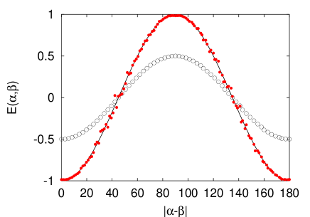
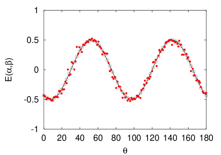
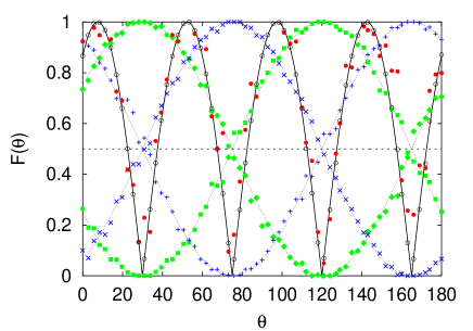
In Fig. 5 (left), we present simulation data for the correlation $E(\alpha,\beta)$ for Case I, that is for the case that the source emits particles with an opposite, random polarization, corresponding to the singlet state in the quantum theoretical description. Figure 5 (right), shows the corresponding results for Case II. It is clear that in both cases, the agreement between the simulation data and quantum theory is excellent.

Also shown in Fig. 5 are the results for $E(\alpha,\beta)$ if we ignore the time-delay data (equivalent to $d=0$ or $W\rightarrow\infty$). In Case I we obtain simulation results that agree very well with the expression $E(\alpha,\beta)=-(1/2)\cos 2\theta$ (see Eq.(33)), a result that differs from what is obtained by considering the class of models studied by Bell Bell (1993). In the latter case an equilateral saw-tooth function is obtained instead of the cosine. In Case II, the results for $d=4$ and $d=0$ or $W\rightarrow\infty$ are, apart from statistical fluctuations, the same. Hence, for Case II the time window $W$ can be omitted for the calculation of the two-particle correlation function.

Figure 5: (color online) Correlation $E(\alpha,\beta)$ between the coincidence counts as a function of the orientation difference of the two polarizers in each observation station. Left: Computer simulation of Case I in which the source emits particles with opposite random polarization (EPRB experiment). Right: Computer simulation of Case II in which the source emits particles with fixed polarization and $\alpha=\theta$, $\beta=\theta+\pi/4$, $\eta_{1}=\pi/6$, and $\eta_{2}=\pi/6+\pi/2$ (see Fig. 2). Squares (red): Simulation results using the time-delay mechanism (with $d=4)$ to compute the two-particle coincidence. Open circles (black): Simulation results without using the time-tags (equivalent to $d=0$ or $W\rightarrow\infty$). Solid lines: Quantum theory.

Figure 6: (color online) Left: Computer simulation of Case I in which the source emits particles with opposite random polarization (EPRB experiment). Right: Computer simulation of Case II in which the source emits particles with fixed polarization. Squares (red): Simulation results for $F(\theta)=|S(\theta)|$ using the time-delay mechanism ($d=4)$. Open circles (black): Simulation results for $F(\theta)=|S(\theta)|$ without using the time-tags (equivalent to $d=0$ or $W\rightarrow\infty$). Other markers: Average single-particle counts on the detectors (see Fig. 1). Squares (green): $F(\theta=\theta_{1})=P_{+}(\theta_{1})$; Diamonds (green): $F(\theta=\theta_{1})=P_{-}(\theta_{1})$; Plusses (blue): $F(\theta=\theta_{2})=P_{+}(\theta_{2})$; Crosses (blue): $F(\theta=\theta_{2})=P_{-}(\theta_{2})$. In Case I (left), these four symbols lie on top of each other. In Case II (right), these markers show the typical Malus law behavior. Solid line: Quantum theory for $|S(\theta)|$. Dashed line at $|S(\theta)|=2\sqrt{2}$: Maximum of $S(\theta)$ if the system is described by quantum theory. Dashed line at $|S(\theta)|=2$: Maximum of $S(\theta)$ if the system is described by the class of models introduced by Bell Bell (1993); Dashed line at $|S(\theta)|=1/2$: Expected number of $+1$ and $-1$ events recorded by the detectors if the input to the polarizers consists of particles with random polarization. Dotted lines: Quantum theory for $P_{+}(\theta_{1})$, $P_{-}(\theta_{1})$, $P_{+}(\theta_{2})$ and $P_{-}(\theta_{2})$.

Figure 7: (color online) Left: Same as Fig. 6 (left) except that $d=2$. Dotted line: $F(\theta)=|S(\theta)|$ calculated from Eq.(33). Right: Same as Fig. 6 (left) except that $d=6$. Dotted line: $F(\theta)=|S(\theta)|$ calculated from Eq.(33).

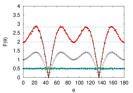
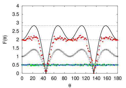
In Fig. 6 (left), we present additional simulation data for Case I. It is clear that for $d=4$, the simulation model reproduces the results of quantum theory for the single-particle expectation values $P_{\pm}(\alpha)$ and $P_{\pm}(\beta)$ (see Table 1) and $S(\theta)$ (see Eq. (9)). Indeed, the frequency with which each detector fires is approximately one-half and $|S(\theta)|$ agrees with the expressions $E(\alpha,\beta)=-\cos 2(\alpha-\beta)$ that is obtained for the singlet state. Also shown in Fig. 6 (left) are the results for $|S(\theta)|$ if we ignore the time-tag data. Effectively, this is the same as letting the time window $W\rightarrow\infty$ or setting $d=0$. Then, our simulation model generates data that satisfies $|S(\theta)|\leq 2$, which is what we expect for the class of models studied by Bell Bell (1993).

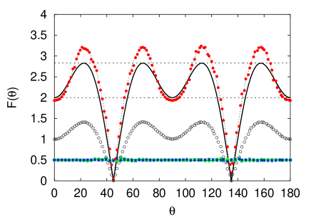
In Case II, the source emits particles with a fixed (but not necessarily opposite) polarization. In the right panel of Fig. 6, we present results for the case $\theta_{1}=\alpha=\theta$ and $\theta_{2}=\beta=\theta+\pi/4$. The angle $\xi$ of the particles is $\pi/6$ (corresponding to $\eta_{1}=\pi/6$ and $\eta_{2}=\pi/6+\pi/2$ in the quantum theoretical description). For this choice, we have $P_{+}(\alpha)=\cos^{2}(\theta-\pi/6)$, $P_{+}(\beta)=\cos^{2}(\theta-\pi/6-\pi/4)$, $E(\alpha,\beta)=2^{-1}\sin 4(\pi/6-\theta)$ and $S(\theta)=\sin 4(\pi/6-\theta)$. Also seen from Fig. 6 (right) is that $|S(\theta)|$ does not depend on $d$, that is apart from statistical fluctuations, the time-tag data do not affect $|S(\theta)|$.

From Fig. 6, it is clear that for $d=4$, the event-by-event simulation model reproduces the single- and two-particle results of quantum theory for both Case I and II, without any change to the algorithm that simulates the polarizers.

Having established that the data generated by our “non-quantum” system agrees with quantum theory, it is of interest to explore if these algorithms can generate data that is not described by quantum theory and by the locally causal, probabilistic models introduced by Bell Bell (1993). We can readily give an affirmative answer to this question by repeating the simulations for Case I (see Fig. 6 (left)) for different values of the time-delay parameter $d$, all other parameters being the same as those used to obtain the data presented in Fig. 6.

For $d=0$, simulations with or without time-delay mechanism yield data that, within the usual statistical fluctuations, are the same (results not shown) and satisfy $|S(\theta)|\leq 2$ . Figure 7 shows the simulation data for $d=2$ and $d=6$. For $0<d<4$ our model yields two-particle correlations that are stronger than those of the Bell-type models but they are weaker than in the case of the singlet state in quantum theory. Therefore, the maximum of $S(\theta)$ is less than $2\sqrt{2}$ but larger than two. For $d\geq 5$, we find that the two-particle correlations are significantly stronger than in the case of the singlet state in quantum theory.

For $d<4$, $2\leq S_{max}<2\sqrt{2}$ for any value of $W/\tau$. Hence, for $d<4$ our model cannot produce the correlations of the singlet state. For $d=4$, $2\leq S_{max}\leq 2\sqrt{2}$ and our model produces the correlations of the singlet state if $W$ is sufficiently small such that contributions of order $W^{2}$ can be negelected. For $d>4$, $2\leq S_{max}\leq 4$, and for a range of $W/\tau$, $S_{max}>2\sqrt{2}$, implying that our model exhibits correlations that cannot be described by the quantum theory of two spin-1/2 particles, while still satisfying Einstein’s criteria for local causality.

From Fig. 7 it can be seen that for $d=2$ and $d=6$ there is good agreement between the results obtained with our event-based simulation model and the analytical result for $|S(\theta)|$ obtained from Eq. (33). For $d=2$, the simulation results show larger fluctuations than for $d=6$, but in all cases these fluctuations can be reduced by increasing $N$ (results not shown).

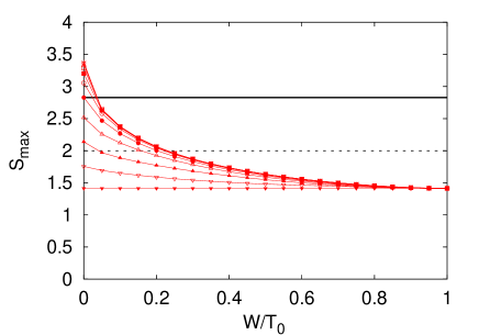
The simulation results presented in Figs. 6 and 7 have been obtained for $W/\tau=1$ and small $\tau$ (recall that the unit of time in our numerical work is set equal to one). In general, in experiment the two-particle correlation depends on both $W$ and $\tau$. Our simulation model makes definite predictions for this dependence. This can be seen from Fig. 8, showing $S_{max}=\max_{\alpha,\alpha^{\prime},\beta,\beta^{\prime}}S(\alpha,\alpha^{\prime},\beta,\beta^{\prime})$ as a function of $W/T_{0}$ for various values of $d$ and of $S_{max}$ to first order in $W$ as a function of $d$. The numerical results agree with the values of $S_{max}$ that have been obtained analytically to first order in $W$, $d=0,2,...,8$ and for $W\rightarrow\infty$.

Figure 8: (color online) Left: $S_{max}=\max_{\alpha,\alpha^{\prime},\beta,\beta^{\prime}}S(\alpha,\alpha^{\prime},\beta,\beta^{\prime})$ as a function of the time window $W$ relative to the maximum time delay resolution $T_{0}$. Curves from bottom to top: Results for $d=0,1,\ldots,10$. Solid line at $2\sqrt{2}$: Value of $S_{max}$ for a quantum system in the singlet state. Dashed line at $2$: Value of $S_{max}$ for a quantum system in an uncorrelated state. Right: $S_{max}=\max_{\alpha,\alpha^{\prime},\beta,\beta^{\prime}}S(\alpha,\alpha^{\prime},\beta,\beta^{\prime})$ as a function of the time-delay parameter $d$ negelecting contributions of ${\cal O}(W)$. Solid line at $2\sqrt{2}$: Value of $S_{max}$ for a quantum system in the singlet state. Dashed line at $2$: Value of $S_{max}$ for a quantum system in an uncorrelated state.

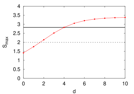
Summarizing: In the regime of small $W/T_{0}=\tau/T_{0}$, the results produced by the simulation algorithm are in excellent agreement with the quantum theoretical expressions (see Table 1) of the single- and two-particle averages.

VIII Comparison with experimental data

For the simulation model described in Section V, it follows immediately from Eqs. (2) and (II) that $|E(\alpha,\beta)|<1$ and that

$$|E(\alpha,\beta)-E(\alpha,{\beta}^{\prime})+E({\alpha}^{\prime},\beta)+E({\alpha}^{\prime},{\beta}^{\prime})|\leq 4.$$ (38)

Without any further constraints on the algorithm that generates the data $\{\Upsilon_{1},\Upsilon_{2}\}$ the upperbound (4) in Eq. (38) cannot be improved. On the other hand, for a local realist (probabilistic) model, it can be shown that Larsson and Gill (2004)

$$|E(\alpha,\beta)-E(\alpha,{\beta}^{\prime})+E({\alpha}^{\prime},\beta)+E({\alpha}^{\prime},{\beta}^{\prime})|\leq\frac{6}{\gamma}-4,$$ (39)

where $\gamma$ is the infimum of the probability of coincidence over all possible settings $\{\alpha,\beta\}$. In our simulation model the frequency of coincidences

$$\Gamma=\frac{1}{N}\sum_{n=1}^{N}\Theta(W-|t_{n,1}-t_{n,2}|),$$ (40)

is easy to compute and, assuming that the results that we obtain by using pseudo-random numbers can be described by a probabilistic model (see Section VI), we may assume that $\gamma=\Gamma$ with probability one. For $W=\tau$ and $d=4$, a straightforward calculation gives

$$\gamma=\min_{\alpha-\beta}\Gamma=\frac{16}{3\pi}\frac{W}{T_{0}}+{\cal O}(W^{2}),$$ (41)

showing that up to first order in the time window $W$, the minimum frequency of coincidences is proportial to the time window, as one naively would expect.

As pointed out in Ref. Larsson and Gill (2004), a local realist model that uses coincidence in time to decide which particles form a pair is not necessarily in conflict with the predictions of quantum theory unless $\gamma>3-3/\sqrt{2}$. Thus, in Case I, it is of interest to explore how $\Gamma$ affects $S_{max}$ and the sinusoidal shape of the two-particle correlation but before we present some results, we want to draw attention to the fact that the model that we introduce in this paper is not unique in the sense that it is not the only model that reproduces the results of quantum theory for the singlet state De Raedt et al. (2006). Different models will yield different numerical results for $\Gamma$ but the general behavior is the same. In these event-based models, there are three independent parameters that we can use to “tune” the simulation results to experimental data, namely $\tau/T_{0}$, $W/T_{0}$, and $d$.

First, we consider the problem of “fitting” our model to experimental data for $S_{max}$. As explained earlier, to obtain $S_{max}$, one has to perform four experiments. For instance, Ref. Weihs et al. (1998) reports $S_{max}\approx 2.73$ using $\alpha=\theta_{1}=0,\pi/4$ and $\beta=\theta_{2}=\pi/8,3\pi/8$ and if we make the hypothesis that the frequency of coincidences that we found earlier ($\approx 0.01$ for $\alpha-\beta=\pm\pi/8,-3\pi/8$) is a good estimate for $\gamma$, no conclusion can be drawn from the relevant theoretical bound Eq. (39), other than that this experiment does not rule out a local realist (probabilistic) description Larsson and Gill (2004). The simulation model described in Section V, reproduces the experimental result $S_{max}\approx 2.73$ Weihs et al. (1998) for $\tau/T_{0}=1/29$, $W/T_{0}=1/29$, and $d=4$. For $\alpha-\beta=0,\pi/8,\pi/4,3\pi/8,\pi/2$ we find $\Gamma=0.38,0.14,0.06,0.14,0.38$, respectively. Because in our simulation the source only emits particle pairs and since no particles are lost or falsely detected, we may expect that the simulation for $\alpha-\beta=\pm\pi/8,-3\pi/8$ yields a value of $\Gamma$ that is larger than the one ($\approx 0.01$) extracted from the experimental data Weihs et al. (1998). A simulation run with N=300000 events (roughly the same number as observed in the experimental data analyzed in Section IV), gives $\sum_{n}x_{n,1}=0.0016,-0.0011$ for $\alpha=0,\pi/4$ and $\sum_{n}x_{n,2}=0.007,0.001$ for $\beta=\pi/8,3\pi/4$, respectively, in reasonable agreement with the experimental results (see Section IV).

For comparison, the simulation model introduced in Ref. De Raedt et al. (2006) reproduces the same value of $S_{max}$ for $\tau/T_{0}=1/9$, $W/T_{0}=1/9$, and $d=2$, yielding $\Gamma=0.38,0.18,0.13,0.18,0.38$ for $\alpha-\beta=0,\pi/8,\pi/4,3\pi/8,\pi/2$, respectively.

As another example, we consider the result $S_{max}\approx 2.25$ as obtained from ion-trap experiments Rowe et al. (2001). Although it is not evident that the events registered in this experiment are as simple as the detection of single photons, let us assume that the model for the real EPRB experiment with photons can nevertheless be used to describe the outcome of these ion-trap experiments. Then, the simulation model described in Section V reproduces the value of $S_{max}\approx 2.25$ if we take $\tau/T_{0}=1/4.3$, $W/T_{0}=1/4.3$, and $d=4$. For $\alpha-\beta=0,\pi/8,\pi/4,3\pi/8,\pi/2$ we find $\Gamma=0.65,0.46,0.32,0.46,0.65$, respectively. For comparison, the simulation model described in Ref. De Raedt et al. (2006) yields the same value of $S_{max}=2.25$ for $\tau/T_{0}=1/1.031$, $W/T_{0}=1/1.031$, and $d=2$, with $\Gamma=0.95,0.89,0.89,0.89,0.95$ for $\alpha-\beta=0,\pi/8,\pi/4,3\pi/8,\pi/2$, respectively. As $\Gamma\approx 1$, this experiment seems to have an almost ideal detection efficiency Rowe et al. (2001).

For completeness, we consider the case $S_{max}=2.83$. Recall that both the model introduced in this paper and the one of Ref. De Raedt et al. (2006) reproduce the result ($E(\alpha-\beta)=-\cos 2(\alpha-\beta)$) of quantum theory if we keep the contributions of ${\cal O}(W)$ only. The model described in Section V yields $S_{max}=2.83$ if we take $\tau/T_{0}=1/1500$, $W/T_{0}=1/1500$, and $d=4$ for which $\Gamma=0.13,0.0032,0.0011,0.0032,0.13$ for $\alpha-\beta=0,\pi/8,\pi/4,3\pi/8,\pi/2$, respectively. For these choices of parameters, the numerical results for $E(\alpha-\beta)$ are very close to those of quantum theory (see Fig. 5).

For the model of Ref. De Raedt et al. (2006) and $\tau/T_{0}=1/1500$, $W/T_{0}=1/1500$, and $d=2$, we find $\Gamma=0.031,0.0011,0.00085,0.0011,0.031$ for $\alpha-\beta=0,\pi/8,\pi/4,3\pi/8,\pi/2$, respectively.

Figure 9: (color online) Left: The frequency of coincidences $\Gamma$ as a function of $|\alpha-\beta|$ for parameters $\tau/T_{0}$, $W/T_{0}$ and $d$ chosen such (see text) that the simulation model reproduces quantum theory (solid line, red), $S_{max}=2.83$, and the values of $S_{max}=2.25$ (dashed line, black) and $S_{max}=2.73$ (dotted line, blue), as obtained from experiments with ions Rowe et al. (2001) and with photons Weihs et al. (1998), respectively. Right: Simulation results of the two-particle correlation $E(\alpha-\beta)$ as a function of $|\alpha-\beta|$ for the model parameters that yield $S_{max}=2.25$ (squares, black) and $S_{max}=2.73$ (stars, blue), respectively. The dashed lines are given by $-0.875\cos 2(\alpha-\beta)$ and $-0.725\cos 2(\alpha-\beta)$. The solid line (red) is the result $-\cos 2(\alpha-\beta)$ of quantum theory (see Fig. 5 (left)).

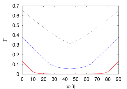
In Fig. 9(left), we plot $\Gamma$ as a function of $\alpha-\beta$, as obtained for the simulation model introduced in the paper, for the three cases $S_{max}=2.25,2.73,2.83$ discussed earlier. The general trend is clear: $\Gamma$ reaches its maximum at $\alpha-\beta=0,\pi/2,\ldots$ and its (nonzero) minimum at $\alpha-\beta=\pi/4,3\pi/2,\ldots$.

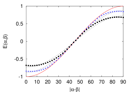
Finally, we study how $E(\alpha-\beta)$ deviates from the result $E(\alpha-\beta)=-\cos 2(\alpha-\beta)$ of a system in the singlet state as we fit the values of $S_{max}$ to the experimental results. In Fig. 9(right), we show the simulation results for the two cases $S_{max}=2.25,2.73$, corresponding to the experiment with ions of Ref. Rowe et al. (2001) and the experiment with photons of Ref. Weihs et al. (1998), respectively. From Fig. 9(right), we see that the main effect of reducing $S_{max}$ is to reduce the amplitude (visibility) of the correlation. Although it is clear that the simulation data cannot be described by a single sinusoidal function, the deviations are small and it remains to be seen if experiments can resolve such small differences.

As is evident from Fig. 8, for $d>4$ our model yields the value for the singlet state $S_{max}=2\sqrt{2}$ without having to consider the regime of small $W$. Thus, in order for an experiment and a model of the type considered in our paper to reproduce the features of a quantum system of two $S=1/2$ particles in the singlet state, it is not sufficient to show that it can yield $S_{max}=2\sqrt{2}$ for some choice of the parameters. As mentioned earlier, the singlet state is completely characterized by the single- and two-particle expectation values. Hence, in order to make a comparison with the singlet state, it is necessary to measure or compute these two quantities.

IX Discussion

We have presented a computer algorithm that simulates Aspect-type EPRB experiments. In the simulation, the source produces particles with opposite but otherwise unpredictable polarization. Each particle of a pair is analyzed in an observation station, consisting of a polarizer and two detectors (Case I). Placing an additional polarizer in between the source and each observation station changes the opposite, unpredictable polarization of the two particles into a pair of fixed, but not necessarily opposite, polarizations (Case II). The time-tag data of the detection events observed in both stations are used for pair identification. Application of quantum theory to both types of experiments yields the single-particle and two-particle expectation values that are characteristic for the singlet state (Case I) and the product state (Case II).

The salient features of the simulation model are that:

• Every essential component of the real laboratory experiment (polarizers, detectors, time-tag logic, data analysis procedure) has a counterpart in the algorithm.

• Identical elements in the experimental setup are represented by identical algorithms. For instance, to simulate Case I and II, we use the same algorithm to simulate the polarizers. In particular, the algorithm that simulates the polarizer reproduces Malus law, which is not essential to reproduce the quantum theoretical results of Case I, see the model introduced in Ref. De Raedt et al. (2006).

• It is event-based and strictly satisfies Einstein’s criteria of local causality but it is not unique.

• At any time, it allows free choice of the directions in which the polarization will be measured, in contrast to laboratory experiments in which the polarizers in the observation stations can take $2\times 2$ directions only Weihs et al. (1998).

• It identifies pairs based on the time-tag of each detection event, using a time window $W$ and allowing for several different procedures to define which two photons form a pair, just as in real laboratory experiments.

• To first order in the time window $W$, it reproduces exactly the single-particle averages and two-particle correlations of quantum theory for both Case I and II.

• It provides information about the frequency of coincidences $\Gamma$. In order to reproduce the results of the two-particle correlation as given by quantum theory for Case I, $\Gamma$ must be sufficiently small. Values of $\Gamma$, corresponding to those found in EPRB laboratory experiments Weihs et al. (1998); Rowe et al. (2001) can be reproduced also. For these values of $\Gamma$, the two-particle correlation function deviates from the quantum theoretical result but the deviations are small. In all cases, the simulation model reproduces the single-particle averages as given by quantum theory.

In our simulation model, the time-tag data are a key element for producing the single-particle expectation values and two-particle correlations as given by the quantum theory of a system of two $S=1/2$ spins. In our model, in Case I, the two-particle correlation depends on the value of the time window $W$. By reducing $W$ from infinity to zero, this correlation changes from typical Bell-like to singlet-like, without making any change to the whole algorithm. Thus, the character of the correlation not only depends on the whole experimental setup but also on the way the data analysis is carried out. Hence, from the two-particle correlation itself, one cannot make any definite statement about the character of the source. Thus, the correlation is a property of the whole system (which is what quantum theory describes), not a property of the source itself. It is of interest to note that if we perform a simulation of Case II the single-particle and two-particle correlations do not depend on the value of the time window $W$. In this case, the observation stations always receive particles with the same polarization and although the number of coincidences decreases with $W$ (and the statistical fluctuations increase), the functional form of the correlation does not depend on $W$.

Summarizing: We have demonstrated that a simulation model that strictly satisfies Einstein’s criteria of locality can reproduce, event-by-event, the quantum theoretical results for EPRB experiments with photons, without using any concept from quantum theory. We have given a rigorous proof that this model reproduces the single-particle expectations and the two-particle correlation of two $S=1/2$ particles in the singlet state and product state.

References

- Einstein et al. (1935) A. Einstein, A. Podolsky, and N. Rosen, Phys. Rev. 47, 777 (1935).
- Bohm (1951) D. Bohm, Quantum Theory (Prentice-Hall, New York, 1951).
- Freedman and Clauser (1972) S. J. Freedman and J. F. Clauser, Phys. Rev. Lett. 28, 938 (1972).
- Aspect et al. (1982a) A. Aspect, P. Grangier, and G. Roger, Phys. Rev. Lett. 49, 91 (1982a).
- Aspect et al. (1982b) A. Aspect, J. Dalibard, and G. Roger, Phys. Rev. Lett. 49, 1804 (1982b).
- Tapster et al. (1994) P. R. Tapster, J. G. Rarity, and P. C. M. Owens, Phys. Rev. Lett. 73, 1923 (1994).
- Tittel et al. (1998) W. Tittel, J. Brendel, H. Zbinden, and N. Gisin, Phys. Rev. Lett. 81, 3563 (1998).
- Weihs et al. (1998) G. Weihs, T. Jennewein, C. Simon, H. Weinfurther, and A. Zeilinger, Phys. Rev. Lett. 81, 5039 (1998).
- Weihs (2000) G. Weihs, Ph.D. thesis, University of Vienna (2000), http://www.quantum.univie.ac.at/publications/thesis/gwdiss.pdf.
- Rowe et al. (2001) M. A. Rowe, D. Kielpinski, V. Meyer, C. A. Sackett, W. M. Itano, C. Monroe, and D. J. Wineland, Nature 401, 791 (2001).
- Fatal et al. (2004) D. Fatal, E. Diamanti, K. Inoue, and Y. Yamamoto, Phys. Rev. Lett. 92, 037904 (2004).
- Sakai et al. (2006) H. Sakai, T. Saito, T. Ikeda, K. Itoh, T. Kawabata, H. Kuboki, Y. Maeda, N. Matsui, C. Rangacharyulu, M. Sasano, et al., Phys. Rev. Lett. 97, 150405 (2006).
- Home (1997) D. Home, Conceptual Foundations of Quantum Physics (Plenum Press, New York, 1997).
- Larsson and Gill (2004) J. A. Larsson and R. D. Gill, Europhys. Lett. 67, 707 (2004).
- De Raedt et al. (2006) K. De Raedt, K. Keimpema, H. De Raedt, K. Michielsen, and S. Miyashita, Euro. Phys. J. B 53, 139 (2006).
- (16) This procedure was suggested to us by R. Gill.
- Bell (1993) J. S. Bell, Speakable and unspeakable in quantum mechanics (Cambridge University Press, Cambridge, 1993).
- Santos (2005) E. Santos, Phil. Mod. Phys. 36, 544 (2005).
- Ẑukowksi (2005) M. Ẑukowksi, Stud. Hist. Phil. Mod. Phys. 36, 566 (2005), arXiv: quant-ph/0605034.
- Gill (2003) R. D. Gill, in Proc. of “Foundations of Probability and Physics - 2”, Ser. Math. Modelling in Phys., Engin., and Cogn. Sc. (Växjö University Press, Växjö, 2003), vol. 5, pp. 179 – 206, arXiv: quant-ph/0301059.
- De Raedt et al. (2007a) H. De Raedt, K. De Raedt, K. Michielsen, K. Keimpema, and S. Miyashita, J. Phys. Soc. Jpn. 76, 104005 (2007a).
- De Raedt et al. (2007b) K. De Raedt, H. De Raedt, and K. Michielsen, Comp. Phys. Comm. 176, 642 (2007b).
- De Raedt et al. (2007c) H. De Raedt, K. De Raedt, K. Michielsen, K. Keimpema, and S. Miyashita, J. Comp. Theor. Nanosci. 4, 1 (2007c).
- Clauser and Horne (1974) J. F. Clauser and M. A. Horne, Phys. Rev. D 10, 526 (1974).
- Clauser et al. (1969) J. F. Clauser, M. A. Horne, A. Shimony, and R. A. Holt, Phys. Rev. Lett. 23, 880 (1969).
- (26) http://www.quantum.at/research/photonentangle/bellexp/data.html. The results presented here have been obtained by assuming that the data sets *_V.DAT contain IEEE-8 byte (instead of 8-bit) double-precision numbers and that the least significant bit in *_C.DAT specifies the position of the switch instead of the detector that fired.
- Cirel’son (1980) B. S. Cirel’son, Lett. Math. Phys. 4, 93 (1980).
- Born and Wolf (1964) M. Born and E. Wolf, Principles of Optics (Pergamon, Oxford, 1964).
- Grimmet and Stirzaker (1995) G. R. Grimmet and D. R. Stirzaker, Probability and Random Processes (Clarendon Press, Oxford, 1995).
- Jaynes (2003) E. T. Jaynes, Probability Theory: The Logic of Science (Cambridge University Press, Cambridge, 2003).
- Ballentine (2003) L. E. Ballentine, Quantum Mechanics: A Modern Development (World Scientific, Singapore, 2003).