On Evolutionary Spatial Heterogeneous Games
Abstract
How coperation between self-interested individuals evolve is a crucial problem, both in biology and in social sciences, that is far from being well understood. Evolutionary game theory is a useful approach to this issue. The simplest model to take into account the spatial dimension in evolutionary games is in terms of cellular automata with just a one-parameter payoff matrix. Here, the effects of spatial heterogeneities of the environment and/or asymmetries in the interactions among the individuals are analysed through different extensions of this model. Instead of using the same universal payoff matrix, bimatrix games in which each cell at site (,) has its own different ‘temptation to defect’ parameter are considered. Firstly, the case in which these individual payoffs are constant in time is studied. Secondly, an evolving evolutionary spatial game such that =, i.e. besides depending on the position evolves (by natural selection), is used to explore the combination of spatial heterogeneity and natural selection of payoff matrices.
keywords:
Complex adaptive systems , Evolutionary Game Theory , Cellular Automata1 Introduction
Cooperation is ubiquitous in nature [1] and essential for evolution [2]. How did cooperative behaviour evolve among self-interested individuals is an important open question in biology and social sciences. A powerful tool to analyse this issue is evolutionary game theory [3]-[5]. It originated as an application of the mathematical theory of games to biological contexts, has become of increased interest to economists, sociologists, and anthropologists as well as philosophers. Of particular interest are two-player games where each player has a strategy space containing two actions or ‘22 games’. In the problem of cooperation vs. competition the two actions or strategies are: to cooperate (C) or to defect (D). The payoff of a player depends on its action and the one of its coplayer. Assuming symmetry between the two players, i.e. that they are interchangable, there are four possible values for this payoff , , & , corresponding respectively to the four situations [C,C], [C,D], [D,C] & [D,D] (the first entrance correspond to the action of the player and the second to the action of its opponent). The paradigmatic example is the Prisoner’s Dilemma (PD) in which the four payoff are ranked as . So is the ‘temptation’ to defect, is the ‘reward’ for mutual cooperation the ‘punishment’ for mutual defection and is the ‘sucker’s payoff’. Clearly it pays more to defect ( and ) but the dilemma is that if both play D they get that is worse than the reward they would have get if they had played C. The PD is connected with two other social dilemma games [6], [7]: When the damage from mutual defection is increased so that it finally exceeds the damage suffered by being exploited, i.e. , the new game is called the chicken [8]. This game applies thus to situations such that mutual defection is the worst possible outcome for both players as it happens in most of animal contests. On the other hand, when the reward surpasses the temptation i.e. , the game becomes the Stag Hunt (SH) [9]. There are several animal behaviours that have been described as stag hunts. For example, the coordination of slime molds. When individual amoebae of Dictyostelium discoideum are starving, they aggregate to form one large body. Here if they all act together they can successfully reproduce, however the success depends on the cooperation of many individuals.
Classical evolutionary game theory constitutes a mean-field approximation which does not include the effect of spatial structures of populations. Axelrod [1] suggested to place the individual “players” in a two-dimensional spatial array playing with its neighbours. These cellular automata (CA) were explored by Nowak and May [10] who use a simple one-parameter payoff matrix specifying a game that is in the frontier between the PD and chicken. They found that the spatial structure allows cooperators to build clusters in which the benefits of mutual cooperation can outweight losses against defectors. This enables the maintenance of cooperation in contrast to the spatially unestructured game where defection is always favoured. Different variations of this Nowak-May (N-M) model were studied taking into account distinct aspects, like the changes introduced by modifying the update rule [11], the effect of allowing voluntary participation [12], the dependence on the graph topology [13],[14], the effect of noise and connectivity structure [15], the consequences of the environmental stress by requiring a minimum threshold to survive [16], etc.
Here my goal is to extend the N-M model in several directions with the aim to study the following issues.
-
1.
The consequences of an heterogeneous environment. This can be modelled through a payoff matrix varying from place to place. For example, in a more hostile region the reward for mutual cooperation can surpass the temptation to defect leading thus to switching from the PD to the SH, etc.
-
2.
The effect of asymmetries in the interactions between the agents. Indeed, asymmetries in the costs and benefits of cooperating have been mentioned as an important ingredient in the evolution of cooperation [17].
-
3.
The emergence of payoff matrices from the very natural selection process. The determination of the ranking of the payoff values to explain the results of experiments or field observations is a far from trivial matter. For instance, in the case of animals there is controversy whether the PD or chicken is the appropriate game [18, 19]. Or many circumstances that have been described as PD might also be interpreted as a SH, depending on how fitness is calculated [9]. Moreover, experimental studies indicate that the payoff matrix is not a constant for very simple individuals like viruses [20].
Hence, the basic idea is, instead of using the same universal payoff matrix, to use heterogeneous bimatrix games [5], i.e. each player has it own particular payoff matrix. I begin studying a first variant of this model, in which the cell payoff matrix is regarded as something completely external to the individual, corresponding to environmental properties. These properties change from place to place but not with time (at least not in the temporal scale of the organisms) and thus the matrix diversity is kept fixed during the evolution.
Then I focus on a second variant in which the cell payoff matrix is assumed to reflect ‘phenotypic’ properties, internal to organisms, thus it evolves together with its strategy.
2 The Model
The N-M model consists in a cellular automaton in which cells represent the simplest possible agents: unconditional players versus its neighbours. That is, at each generation or time step of the game, there are those who always play C and those who always play D. Different types of neighbourhoods can be considered. For example the von Neumann neighbourhood with =4 neighbour cells (above, below, left and right cells). The score of a given player is the sum of the payoffs it collects against its neighbours. The payoff matrix depends on just one parameter while the other three have fixed values: =1, ==0. The dynamic is synchronous: all the agents update their states simultaneously at the end of each lattice sweep 111It is known that synchronous actualisation of the state of a lattice can induce artificial effects. I studied then what happened when performing an asynchronous update i.e. each site is updated after comparing with their neighbourhood. I found qualitatively the same results.. Natural selection is mimicked through the simplest ’Imitate the Best’ (in the neighbourhood) update rule [21] : Each individual, after playing against its neighbours, adopts the strategy of the most successful neighbour or (the one that collected the highest utilities in the neighbourhood at this round).
In this work two variants of the N-M model are studied:
-
•
Heterogeneous non evolving temptation.
As a first step let’s consider the version with the temptation parameter varying from cell to cell as a uniform random variable fixed in time: , where and are the coordinates of the center of the cell. Since =, when 1 the payoff matrix of the cell at (,) is in the frontier between the PD and the chicken, let’s denote this game by . On the other hand, when 1 the game played by the cell is in the frontier between the PD and the SH and let’s denote it by .
-
•
Heterogeneous evolving temptation.
Next I concentrate on the case in which the temptation , besides varying from cell to cell, evolves with time i.e. we have a variable depending on the cell coordinates as well as the time step or generation . It starts, at =0, as a uniform random variable and then evolves by natural selection: at each generation all the members of a neighbourhood adopt the payoff matrix of the .
Different intervals [,] for are explored. is taken in [1,2.5] in steps of 0.1, and for each of these values two values of are considered: 0 and 1. Since , the possible games are determined by : when =1 the payoff matrix of every cell corresponds to . On the other hand, the case =0 is less restrictive. In some cells the game can be and in others .
Square lattices of sizes ranging from to , with periodic boundary conditions are used.
The initial configuration for strategies is half of the cells, chosen at random, playing C and the other half playing D. The temptation varies from cell to cell as a uniform random variable in the interval [,].
For each generation the average fraction of cooperators and, in the second variant, the average temptation are computed until the steady state is reached (typically, this takes between 500 to 1000 generations). The symbols denote averages that are both spatial, over all the lattice cells, and over 500 runs each starting from a different initial configuration (to ensure independence of the initial conditions).
3 Results
3.1 Heterogeneous non evolving temptation
Both the =4 von Neumann neighbourhood and the =8 Moore neighbourhood were studied producing qualitatively the same results. Therefore, all the results presented in this work are for =4.
Fig. 1 shows the asymptotic values of vs. . To allow comparison with the N-M model we also plot its results (in this case the temptation is the same universal parameter for all the cells i.e. = = ). Roughly the =4 N-M CA exhibits four different regions in the parameter axis, each corresponding to a given different asymptotic value of : 14/3, 4/33/2, 3/22 and 2.
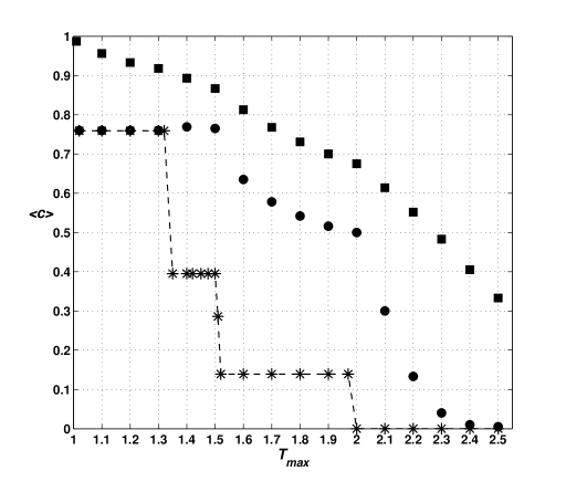
Note that the heterogeneous temptation model yields higher values for the asymptotic fraction of cooperators. For =1 it coincides with the N-M model until =4/3, reproducing its higher step, but then it detaches from it. In the case of =0 the differences are more drastic: no steps are observed, and even for =2.5 there’s cooperation ( 1/3). In fact , as expected, is always greater for =0 since, on average, the temptation to defect is smaller. For example, for =2, when changes from 1 to 0, the fraction of cooperators jumps from 1/2 to 2/3.
3.2 Evolving heterogeneous temptation
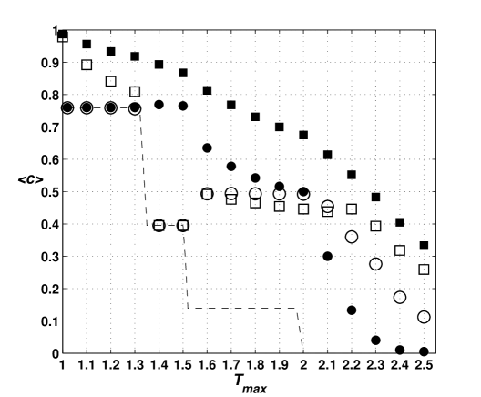
Fig. 2 includes the data of Fig. 1 plus the corresponding asymptotic produced by the evolving temptation variant, for the same values of and . Note that this version yields higher values for the asymptotic fraction of cooperators. For =1 results are even more similar to the ones of the N-M model, there is complete coincidence up to =3/2. When higher values of are allowed, something new occurs: the behaviour becomes non-monotonic, there’s also a step but now higher than the one to the left. This is quite unexpected, because when larger ‘temptation’ values are allowed, the fraction of cooperators becomes also larger. For the steps behaviour disappears. In the case of =0 the points interpolate between the ones of the corresponding heterogeneous non evolving variant and the N-M. In fact, they coincide with the points for =1 over the step [=4/3, =3/2] and also show a non-monotonic variation for 3/2.
In Fig. 3 the evolution of the average temptation and fraction of cooperators for =1 and both for =0 and =1 is shown. As expected, the value of is lower for =0 than for =1. Notice the sort of ’specular symmetry’ between the curves of and when they evolve from =(2-0)/2=1 and =0.5 , respectively, to their steady state values. There is a short transient in which () grows (drops) very quickly and then it decreases (increases) until it reaches its asymptotic value.
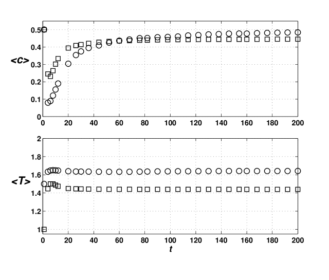
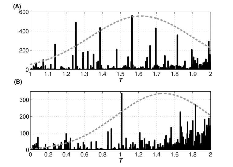
These opposite behaviours are quite surprising since an increase of the average payoff for cheating is accompanied by an increase of the average cooperation level (just the opposite to what happens in the case of non evolving temptation). Besides the average of the temptation , let’s analyse also the evolution of its distribution. Fig. 4 shows the asymptotic (after 200 time steps) distribution of values of the temptation for =2 and for =1 (A) and =0 (B), for a single initial condition. Hence, in both cases there is evolution from a uniform distribution to a non uniform one. The mean value for the temptation produced by these histograms are, respectively, 1.615 and 1.42, both values in good agreement with the asymptotes for in Fig. 3. In the case of =0 a gaussian envelope can be completely discarded (gray dashed curve). For =1 the situation is not so clear.
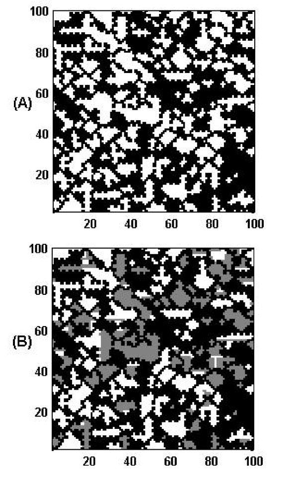
The spatial patterns that emerge are illuminating. For instance, let’s analyse what happens for =2 and =0 for an arbitrary choice of initial conditions. Fig. 5-(A) represents a typical steady state map showing clusters of C agents (white) on a ’sea’ of D agents (black) for a lattice of 100100=10,000 sites. In Fig. 5-(B), all the agents that have a temptation 1= are marked in grey. Notice that they are a subset of the C agents. In other words, all the agents that were selected with low values of are cooperators (the reciprocal is not true: many C agents have values of =1). An explanation for this is that at the end only ”successful” players remain i.e. players whose strategies and phenotypes (temptation ) were copied by its neighbours. A player with a small clearly cannot be successful playing D so it must have been playing C.
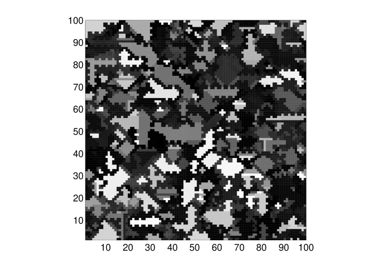
As a result of selection, the system evolves from an initial configuration with different payoff matrices (one per lattice cell) to a situation in which many less matrices coexist. Starting in this case with 100100=10,000 payoff matrices one ends typically with around 500. This is shown in Fig. 6 which is the corresponding map of asymptotic values of . In this particular case it consists in 548 ‘patches’ of different tones of gray, each corresponding to a selected value of . One can recognize several of the domains that appear in Fig. 5-(B). This is natural since the strategy (C or D) of the is copied by agents together with its temptation. Also, it helps to understand why there are no clusters with white and gray sites well mixed in Fig. 5-(B): the typical length of the -patches is much larger than the lattice spacing.
The average individual score can be approximated by
| (1) |
Substituting in equation (1) the computed values of and , one get a value that slightly overestimates . For example, for =4: 0.47 & 0.43.
4 Discussion and Final Comments
Two variants implementing heterogeneous extensions of the N-M model were introduced and studied. These model versions can be regarded as two extreme situations: On the one hand, in the case of ‘temptations’ constant in time, we have the external environment point of view. That is, the payoff matrix is regarded as something completely external to the individuals corresponding to the properties of physical background in which they are located. These properties change from place to place but not with time (at least not in the temporal scale of the organisms) preserving thus the original complete diversity of payoffs. For example, in sites where the environment is more hostile the reward for mutual cooperation may become better than the temptation leading to switching from the PD to the SH, etc. On the other hand, when the temptation evolves, we have the ‘phenotypic’ point of view. In this case, one assumes that the payoff matrix reflects properties of an organism, i.e. is part of its phenotype, so it experiences natural selection. Therefore the model can cope with diversity and asymmetric interactions between ‘players’ either if they are product of an heterogeneous environment or of different ‘phenotypes’ characterized by different temptations . That is, for multiple causes, it is possible that the payoffs for you and your opponent are not equal (indeed this is what happens in general in real life). Furthermore, as it was mentioned, an empirical determination of the payoffs can be very difficult while variations in the payoff values can dramatically alter theoretical predictions. Here, one of my goals was to minimize the dependence of crucial model predictions, like the evolution of cooperation, on model parameters. So I have chosen the simplest agents -unconditional players (without memory or strategic parameters)- and I have not introduced a universal temptation parameter for all the players. Instead, starting with random heterogeneous distributions of , I let that steady states with several domains characterized by different values of emerge from the very process of natural selection. All the results are quite robust and do not depend on particular payoffs choices, nor on the lattice topology or if the update is synchronous or asynchronous, and do not rely on specific characteristics of the agents. The dependence on the initial conditions is also mostly removed by taking averages. Thus this really minimal model seems to combine robustness with realism and simplicity.
Both model variants yield a higher value of the asymptotic fraction of cooperators than the one produced by the uniform N-M model. It is worth remarking that for this heterogeneous payoff matrix model, in general, attains higher values for the the case of constant payoff matrices than for the evolving ones. Also, for both model variants, in general, a diminution of (from 1 to 0) promotes a higher level of cooperation. This seems natural since less competitive games (limit cases of SH) are allowed.
The behaviour of as a function of = is approximately monotonic for constant payoff matrices while in the case of evolving payoff matrices it exhibits non-monotonic variations. So, in this second variant, an interesting (unexpected) prediction is that by allowing larger initial ‘temptation’ payoffs the number of cooperators grows.
Concerning the emergence of spatial patterns, the evolving temptation version organises into a steady state that exhibits a rich structure with several ’patches’ of agents using the same payoff matrix. In addition, all the agents that reach the steady state with values of =1 (when =0) are cooperators.
In this work the evolution is driven just by natural selection. The effect of incorporating mutations, the other driving force of evolution, is something important to explore. Work is in progress on that direction. Nevertheless, preliminary results show that the main conclusions presented here remain qualitatively the same. It is also known that modifications of the update rule, and, in particular, an asynchronous dynamics may produce important changes [11],[14],[21]. The effects of changing the update rule is something that deserves to be analysed separately in another work.
ACKNOWLEDGEMENTS
I would like to thank one of the referees who pointed out the work of M. Perc [22] on heterogeneous games and the effects of additive chaotic variations to the payoff matrix of the spatial PD game. The author proposes that this disturbances can arise either by the player themselves or from the environment, situations that correspond to the two different model variants I study here.
References
- [1] R. Axelrod, in The Evolution of Cooperation, Basic Books, New York, 1984;
- [2] J. Maynard-Smith, and E. Szathmary, The Major Transitions in Evolution, Oxford University Press 1997.
- [3] J. Maynard-Smith, Evolution and the Theory of Games (Cambridge Univ. Press, 1982).
- [4] J. W. Weibull, Evolutionary game theory (MIT Press, 1995).
- [5] J. Hofbauer, K. Sigmund, Evolutionary games and population dynamics (Cambridge University Press, 1998).
- [6] Poundstone, W. Prisoner’s Dilemma, (Doubleday, NY, 1992) 215-217.
- [7] W. M. Liebrand, Simulation Gaming 14, 123 (1983).
- [8] Rapoport, A. Two-Person Game Theory: The Essential Ideas (Ann Arbor: U Michigan, 1966).
- [9] Skyrms, B. :The Stag Hunt and the Evolution of Social Structure (Cambridge University Press 2004).
- [10] M. A. Nowak, R. May, Int. J. Bifurcat. Chaos 3, 35 (1993).
- [11] G. Szabó and C. Toke, Phys. Rev. E 58, 69 (1998).
- [12] G. Szabó and C. Hauert, Phys. Rev. E 66, 062903 (2002).
- [13] G. Abramson and M. Kuperman, Phys. Rev. E 63, 030901 (2001).
- [14] G. Szabó, J. Vukov and A. Szolnoki, Phys. Rev. E 72, 047107 (2005).
- [15] J. Vukov, G. Szabó and A. Szolnoki, Phys. Rev. E 73, 067103 (2006).
- [16] J. Alonso, A. Fernández and H. Fort J. Stat. Mech. (2006) P06013.
- [17] T. Clutton-Brock, Science 296, 69 (2002).
- [18] R. Heinsohn, C. Packer, Science 269, 1260 (1995).
- [19] M. A. Nowak, K. Sigmund, Nature 398, 367 (1999).
- [20] P. E. Turner, L. Chao, The American Naturalist 161, 497 (2003).
- [21] G. Szabó and G. Fáth, Physics Reports 446, 97 (2007).
- [22] M. Perc, Europhysics Letters 75, 841 (2006); New J. Phys. 8, 183 (2006).