Single-Sweep Methods for Free Energy Calculations

Abstract

A simple, efficient, and accurate method is proposed to map multi-dimensional free energy landscapes. The method combines the temperature-accelerated molecular dynamics (TAMD) proposed in [Maragliano & Vanden-Eijnden, Chem. Phys. Lett. 426, 168 (2006)] with a variational reconstruction method using radial-basis functions for the representation of the free energy. TAMD is used to rapidly sweep through the important regions of the free energy landscape and compute the gradient of the free energy locally at points in these regions. The variational method is then used to reconstruct the free energy globally from the mean force at these points. The algorithmic aspects of the single-sweep method are explained in detail, and the method is tested on simple examples, compared to metadynamics, and finally used to compute the free energy of the solvated alanine dipeptide in two and four dihedral angles.

I Introduction

The free energy (or potential of mean force) is the thermodynamic force driving structural processes such as conformational changes of macromolecules in aqueous solution, ligand binding at the active site of an enzyme, protein-protein association, etc. The free energy gives information about both the rate at which these processes occur and the mechanism by which they occur. This makes free energy calculations a central issue in biophysics. Molecular dynamics (MD) simulations provide a tool for performing such calculations on a computer in a way which is potentially both precise and inexpensive (e.g. fe1 ; fe2 ; fe3 ). Since a free energy is in essence the logarithm of a probability density function (see (1) below for a precise definition) it can in principle be calculated by histogram methods based on the binning of an MD trajectory. This direct approach, however, turns out to be unpractical in general because the time scale required for the trajectory to explore all the relevant regions of configuration space is prohibitively long. Probably the best known and most widely used technique to get around this difficulty is the weighted histogram analysis method (WHAM) wham . Following valleau , WHAM adds artificial biasing potentials to maintain the MD system in certain umbrella sampling windows. WHAM then recombines in an optimal way the histograms from all the biased simulations to compute the free energy. WHAM is much more efficient than the direct sampling approach, and generalizations such as karplus alleviate somewhat the problem of where to put the umbrella windows (usually, this requires some a priori knowledge of the free energy landscape). In practice, however, WHAM remains computationally demanding and it only works to compute the free energy in 2 or 3 variables. An interesting alternative to WHAM is metadynamics Laio02 ; Laio03 . In essence metadynamics is a way to use an MD trajectory to place inverted umbrella sampling windows on-the-fly and use these windows both to bias the MD simulation and as histogram bins to sample the free energy directly (thereby bypassing the need of further histogram analysis in each window).

Both WHAM and metadynamics compute the free energy directly by histogram methods, but an alternative approach is possible. Unlike the free energy which is a global quantity, its negative gradient (known as the mean force) can be expressed in terms of a local expectation and thereby computed at a given point in the free energy landscape. This is the essence of the blue moon sampling strategy BlueM99 and it offers the possibility to calculate first the mean force at a given set of locations, then use this information to reconstruct the free energy globally. In one dimension, this approach is known as thermodynamic integration and it goes back to Kirkwood kirkwood . In higher dimensions, however, this way to compute free energies has been impeded by two issues. The first is where to place the points at which to compute the mean force, and the second is how to reconstruct the free energy from these data

In this paper, we propose a method, termed single-sweep method, which addresses both of these issues in two complementary but independent steps. In a first step, we use the temperature-accelerated molecular dynamics (TAMD) proposed in tamd (see also varo02 ; Tuck01 ) to quickly sweep through the important regions of the free energy landscape and identify points in these regions where to compute the mean force. In the second step we then reconstruct the free energy globally from the mean force by representing the free energy using radial-basis functions, and adjusting the parameters in this representation via minimization of an objective function.

The single-sweep method is easy to use and implement, does not require a priori knowledge of the free energy landscape, and can be applied to map free energies in several variables (up to four, as demonstrated here, and probably more). The single-sweep method is also very efficient, especially since the mean force calculations can be performed using independent calculations on distributed processors (i.e. using grid computing facilities grid1 ; grid2 ).

The reminder of this paper is organized as follows. In Sec. II, we describe the two steps of the single-sweep method in detail, starting with the second one for convenience. In Sec. III we illustrate the method on a simple two-dimensional example. This example is then used for comparison with metadynamics in Sec. IV. In Sec. V we use the single-sweep method to compute the free energy of alanine dipeptide (AD) in solution in two and in four of its dihedral angles. Finally, concluding remarks are made in Sec. VI and the details of the MD calculation on AD are given in Appendix A

II The Single-Sweep method

II.1 Free energy representation and reconstruction

We shall consider a molecular system with $n$ degrees of freedom whose position in configuration space $\Omega\subseteq\mathbb{R}^{n}$ will be denoted by ${\bm{x}}$. We also introduce a set of $N$ collective variables ${\bm{\theta}}({\bm{x}})=(\theta_{1}({\bm{x}}),\ldots,\theta_{N}({\bm{x}}))$ which are functions of ${\bm{x}}$ such as torsion angles, interatomic distances, etc. If $V({\bm{x}})$ denotes the potential energy of the system and $1/\beta$ its temperature, the free energy $A({\bm{z}})$ in the variables ${\bm{\theta}}({\bm{x}})$ is defined as

$$A({\bm{z}})=-\beta^{-1}\log\int_{\Omega}e^{-\beta V({\bm{x}})}\delta({\bm{\theta}}({\bm{x}})-{\bm{z}})dx$$ (1)

so that $e^{-\beta A({\bm{z}})}$ is, up to a proportionality constant, the probability density function (PDF) of the variables ${\bm{\theta}}({\bm{x}})$.

As mentioned in the introduction, the negative gradient of the free energy, ${\bm{f}}({\bm{z}})=-\nabla_{\!z}A({\bm{z}})$, is known as the mean force, and it can be computed locally at point ${\bm{z}}$ via calculation of an expectation (see (11) below). In this section, we shall suppose that we have obtained an estimate of ${\bm{f}}({\bm{z}})$ at points ${\bm{z}}_{1},\ldots,{\bm{z}}_{K}$, and we focus on the reconstruction of the free energy $A({\bm{z}})$ from these data. A specific way to pick these points and compute ${\bm{f}}_{\!1}\approx{\bm{f}}({\bm{z}}_{1}),\ldots,{\bm{f}}_{\!K}\approx{\bm{f}}({\bm{z}}_{K})$ will be given in Sec. II.2, but it is worth pointing out that the reconstruction method proposed here works with data set collected in any other ways.

Our reconstruction method uses a radial-basis function representation for the free energy $A({\bm{z}})$ with centers at ${\bm{z}}_{1},\ldots,{\bm{z}}_{K}$ radialbasis0 ; radialbasis1 :

$$\tilde{A}({\bm{z}})=\sum_{k=1}^{K}a_{k}\varphi_{\sigma}(|{\bm{z}}-{\bm{z}}_{k}|)+C.$$ (2)

Here $C$ is a constant used to adjust the overall height of $\tilde{A}({\bm{z}})$ but is otherwise irrelevant, $|\cdot|$ denotes the Euclidean norm in $\mathbb{R}^{N}$, and $\varphi_{\sigma}(u)=\varphi(u/\sigma)$ where $\varphi(u)$ is a radial-basis function; a convenient choice is to use the Gaussian packet

$$\varphi(u)=e^{-\frac{1}{2}u^{2}}$$ (3)

though other radial-basis functions (multiquadric, Sobolev splines, Wendland, etc. radialbasis0 ) can be used as well, see Sec. V. In (2) the heights $a_{k}$ and the radial-basis function width $\sigma>0$ are adjustable parameters which we determine by minimizing over $a_{k}$ and $\sigma$ the following objective function, which measures the discrepancy between the negative gradient of the function $\tilde{A}(z)$ in (2) at the centers ${\bm{z}}_{k}$, $\nabla_{z}\tilde{A}({\bm{z}}_{k})=\sum_{k^{\prime}=1}^{K}a_{k^{\prime}}\nabla_{z}\varphi_{\sigma}(|{\bm{z}}_{k}-{\bm{z}}_{k^{\prime}}|)$, and the mean force ${\bm{f}}_{\!k}$ estimated at these centers:

$$E(a,\sigma)=\sum_{k=1}^{K}\Big{|}\sum_{k^{\prime}=1}^{K}a_{k^{\prime}}\nabla_{z}\varphi_{\sigma}(|{\bm{z}}_{k}-{\bm{z}}_{k^{\prime}}|)+{\bm{f}}_{\!k}\Big{|}^{2}.$$ (4)

Before explaining how we perform this minimization, let us give several reasons why the radial-basis representation (2) for $A({\bm{z}})$ is natural and convenient. First, the centers ${\bm{z}}_{k}$ in (2) do not have to lie on a regular grid, which permits to use mean force data collected anywhere. Second, the representation (2) can be used in any dimension. Third, this representation has very good convergence properties, i.e. a small number of centers gives an accurate representation of $A({\bm{z}})$. In fact, unlike standard representations based e.g. on linear interpolation on a regular grid, the rate of convergence in $K$ of the representation in (2) can be made independent of $N$ (a feature which the radial-basis representations share with sparse grids radialbasis2 ; sparsegrid ).

Going back to the minimization of $E(a,\sigma)$, it can be performed as follows. For fixed $\sigma$, the $a^{\star}_{k}$ minimizing (4) solve the following linear algebraic system

$$\sum_{k^{\prime}=1}^{K}B_{k,k^{\prime}}(\sigma)a^{\star}_{k^{\prime}}(\sigma)=c_{k}(\sigma)$$ (5)

where $B_{k,k^{\prime}}(\sigma)$ and $c_{k}(\sigma)$ are given by

$$B_{k,k^{\prime}}(\sigma) =\sum_{k^{\prime\prime}=1}^{K}\nabla_{z}\varphi_{\sigma}(|{\bm{z}}_{k}-{\bm{z}}_{k^{\prime\prime}}|)\cdot\nabla_{z}\varphi_{\sigma}(|{\bm{z}}_{k^{\prime\prime}}-{\bm{z}}_{k^{\prime}}|),$$ (6)

$$c_{k}(\sigma) =-\sum_{k^{\prime}=1}^{K}\nabla_{z}\varphi_{\sigma}(|{\bm{z}}_{k}-{\bm{z}}_{k^{\prime}}|)\cdot{\bm{f}}_{\!k^{\prime}}\,.$$

Given the centers ${\bm{z}}_{k}$ and the estimates ${\bm{f}}_{k}$ of the mean force at these centers, the coefficients $B_{k,k^{\prime}}$ and $c_{k}$ can be easily computed, and the linear system (5) can be solved by any standard technique, e.g. Gaussian elimination. Once the solution $a^{\star}_{k}\equiv a^{\star}_{k}(\sigma)$ of (5) is determined, to find the optimal $\sigma^{\star}$ satisfying $E(a^{\star}(\sigma^{\star}),\sigma^{\star})=\min_{\sigma}E(a^{\star}(\sigma),\sigma)$ we compute the residual $E(a^{\star}(\sigma),\sigma)$ for increasing values of $\sigma$ starting from the distance between the centers. More sophisticated procedures could be used to minimize $E(a^{\star}(\sigma),\sigma)$ over $\sigma$, but the brute force method that we used proved to be efficient enough because computing successive solutions of (5) for various $\sigma$ is very fast. To measure the error in the approximation, we used the residual per center defined as

$$e_{2}(\sigma)=E^{1/2}(a^{\star}(\sigma),\sigma)/K\,,$$ (7)

which reaches its minimum value at the same $\sigma^{\star}$ as $E(a^{\star}(\sigma),\sigma)$.

Overall, the procedure is simple and inexpensive since the determination of $a^{\star}_{k}$ at fixed $\sigma$ is computationally straightforward and cheap, and can be easily repeated to perform the one-dimensional minimization over $\sigma$. One caveat that we should mention, however, is that the condition number of the matrix $B_{k,k^{\prime}}(\sigma)$ increases rapidly when the number of centers and/or $\sigma$ increase. This is a known problem of radial-basis functions radialbasis1 . To avoid any problems, we capped the admissible condition number at $10^{12}$ and, in situations where this threshold value was reached while $e_{2}(\sigma)$ was still decreasing, picked for $\sigma^{\star}$ the corresponding value of $\sigma$. These situations only occurred in the two-dimensional example (see Sec. III) when a lot of centers were used (500 or more, i.e. much more than what will be used in the AD example), and even in these cases, such a large condition number did not lead to any noticeable loss of accuracy in the results (even though the coefficients $a^{\star}_{k}$ were then very large). We also observed that, given a number of centers ${\bm{z}}_{k}$ and a value of $\sigma$, the condition number is typically lower when the dimension of ${\bm{z}}$ is larger. Finally, we observed that the condition number was much lower with the Wendland radial-basis function (see (16) in Sec. V) than with the Gaussian radial-basis function (3).

II.2 TAMD for sweeping

It remains to explain how to identify the centers ${\bm{z}}_{1},\ldots{\bm{z}}_{K}$ and estimate the mean force at these points. Following tamd , we will do so using the extended system

$$\begin{cases}\begin{aligned} M\ddot{\bm{x}}&=-\nabla_{x}V({\bm{x}})-\kappa\sum_{\alpha=1}^{N}(\theta_{\alpha}({\bm{x}})-z_{\alpha})\nabla_{x}\theta_{\alpha}({\bm{x}})\\[-4.0pt] &\quad+\text{thermostat terms at $\beta^{-1}$}\end{aligned}\\[20.0pt] \displaystyle\gamma\dot{\bm{z}}=\kappa({\bm{\theta}}({\bm{x}})-{\bm{z}})+\sqrt{2\gamma\bar{\beta}^{-1}}\,{\bm{\eta}}(t)\end{cases}$$ (8)

where $M$ is the mass matrix, ${\bm{\eta}}(t)$ is a white-noise, i.e. a Gaussian process with mean 0 and covariance $\langle\eta_{\alpha}(t)\eta_{\alpha^{\prime}}(t^{\prime})\rangle=\delta_{\alpha\alpha^{\prime}}\delta(t-t^{\prime})$, and $\kappa>0$, the friction coefficient $\gamma>0$ and the artificial inverse temperature $1/\bar{\beta}\ (\not=1/\beta)$ are parameters whose role we explain now.

The system in (8) describes the motion of ${\bm{x}}$ and ${\bm{z}}$ over the extended potential

$$U_{\kappa}({\bm{x}},{\bm{z}})=V({\bm{x}})+\tfrac{1}{2}\kappa|{\bm{\theta}}({\bm{x}})-{\bm{z}}|^{2}.$$ (9)

As shown in tamd , by adjusting the parameter $\kappa$ so that ${\bm{z}}(t)\approx{\bm{\theta}}({\bm{x}}(t))$ and the friction coefficient $\gamma$ so that ${\bm{z}}$ moves slower than ${\bm{x}}$, one can generate a trajectory ${\bm{z}}(t)$ in $z$-space which effectively moves at the artificial temperature $1/\bar{\beta}$ on the free energy computed at the physical temperature $1/\beta$. By taking $1/\bar{\beta}>1/\beta$, the ${\bm{z}}(t)$ trajectory visits rapidly the regions where the free energy is relatively low (i.e. within a range of a few $1/\bar{\beta}$) even if these regions are separated by barriers which the system would take a long time to cross at the physical temperature $1/\beta$. This gives us a way to determine automatically where are the relevant regions in free energy space.

In tamd , the extended system in (8) was proposed to sample the free energy landscape directly. Here, we make a different use of (8): we utilize the trajectory ${\bm{z}}(t)$ to rapidly sweep through ${\bm{z}}$-space and generate the centers ${\bm{z}}_{1},\ldots,{\bm{z}}_{K}$ used in the radial-basis representation (2). Specifically, we start from ${\bm{z}}(0)={\bm{z}}_{1}$, then deposit a new center ${\bm{z}}_{k}$ along ${\bm{z}}(t)$ each time ${\bm{z}}(t)$ reaches a point which is more than a prescribed distance $d$ away from all the previous centers, where $d$ is a parameter controlling the density of the covering by the centers (the smaller $d$, the higher the number of centers deposited). At the same time, at each of these centers ${\bm{z}}_{k}$, we launch a simulation of (8) with ${\bm{z}}(t)={\bm{z}}_{k}$ fixed, i.e we use

$$M\ddot{\bm{x}} =-\nabla_{x}V({\bm{x}})-\bar{\kappa}\sum_{\alpha=1}^{N}(\theta_{\alpha}({\bm{x}})-z_{k,\alpha})\nabla_{x}\theta_{\alpha}({\bm{x}})$$ (10)

$$\quad+\text{thermostat terms at $\beta^{-1}$}$$

and compute:

$${\bm{f}}_{\!k}=\frac{1}{T}\int_{0}^{T}\bar{\kappa}\left({\bm{z}}_{k}-{\bm{\theta}}({\bm{x}}(t))\right)dt\,.$$ (11)

The calculations of these time averages are independent of each other, and hence they can be distributed, using (ideally) at least one processor per center ${\bm{z}}_{k}$, an approach that optimally fits with the purposes of grid computing grid1 ; grid2 . The estimator in (11) has the advantage of being simple, but it introduces an error due to the finiteness of $\bar{\kappa}$. This error can be decreased by using $\bar{\kappa}$ in (10) and (11) larger than $\kappa$ in (8), or even eliminated by using constrained instead of restrained simulations and using the blue-moon estimator for the mean force chemphyschem ; free_cpam .

Once the centers ${\bm{z}}_{1},\ldots,{\bm{z}}_{k}$ have been deposited and the estimates ${\bm{f}}_{\!1},\ldots,{\bm{f}}_{\!K}$ of the mean force at these centers have been obtained, we use the reconstruction procedure explained in Sec.II.1 and compute the optimal set of coefficients $a^{\star}_{k}$ and the optimal $\sigma^{\star}$ to use in the representation (2) for $A({\bm{z}})$.

We conclude this section by stressing that using the extended dynamics (8) to sweep through ${\bm{z}}$-space and deposit the centers ${\bm{z}}_{k}$ is very different than using it to sample $A({\bm{z}})$ directly, which makes our approach very different from WHAM or metadynamics. Unlike with sampling, revisiting twice a region in ${\bm{z}}$-space is unnecessary and even undesirable since no new center will be deposited. The accuracy of the reconstruction depends on the number of centers and the accuracy at which the mean force is computed in (11) much more than the precise locations where the centers are deposited. An important practical consequence is that it is rather straightforward to pick the parameters $\kappa$ and $\gamma$ in (8) since the final result is robust against variations in these parameters.

Figure 1: A trajectory generated by simulating (12) by forward Euler with a time-step ${\mathit{\Delta}}t=2\cdot 10^{-5}$ for $2\cdot 10^{4}$ steps (white curve) shown above the contour plot of the Mueller potential (with $29$ level sets evenly distributed between $V=0$ and $V=180$ in a scale where the minimum of the potential is $V=0$). The red circles are the locations of the centers deposited along the trajectory using $d=0.175$. In this run, $174$ centers were deposited.

III Two-dimensional illustrative example

Since, given the location of the centers ${\bm{z}}_{k}$, the mean force estimation at these points is quite standard, as a first illustration we use a two-dimensional example for which ${\bm{\theta}}({\bm{x}})\equiv{\bm{x}}=(x,y)$ and $A({\bm{z}})\equiv V({\bm{x}})$ where $V({\bm{x}})$ is the Mueller potential mueller . In this case, there is no need to extend the system as in (8), and the temperature accelerated dynamics simply reduces to (setting $\gamma=1$ by appropriate rescaling of time)

$$\dot{\bm{x}}=-\nabla V({\bm{x}})+\textstyle\sqrt{2\bar{\beta}^{-1}}\,{\bm{\eta}}(t)\,.$$ (12)

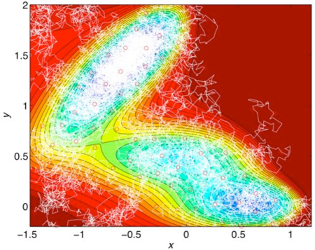
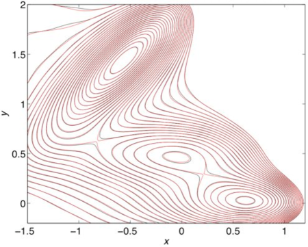
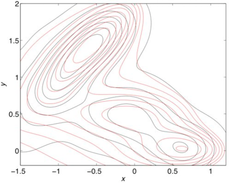
Fig. 1 shows a TAMD trajectory generated by solving (12) by forward Euler with the initial condition $(x(0),y(0))=(1,0)$ and a time-step of $\mathit{\Delta}t=2\cdot 10^{-5}$ for $2\cdot 10^{4}$ time-steps at $1/\bar{\beta}=40$ (for comparison the energy barrier between the two main minima of the Mueller potential is about $100$). Also shown are the centers ${\bm{z}}_{k}\equiv(x_{k},y_{k})$ obtained by depositing a new center along the trajectory each time the trajectory reaches a point which is $d=0.175$ away for all the previous centers. In this run, $174$ centers were deposited. At the centers, we used $-\nabla V(x_{k},y_{k})={\bm{f}}_{\!k}$ as estimate of the “mean force” (i.e. there is no sampling error in the present example). We then used these data to reconstruct the free energy as explained in Sec. II.1. Fig. 2 shows the residual per center $e_{2}(\sigma)$ defined in (7). The optimal $\sigma$ for this run was $\sigma^{\star}=0.398$ and the condition number at this $\sigma^{\star}$ was $7\cdot 10^{6}$. The level sets of the reconstructed potential are shown in Fig. 3 and compared to those of the original Mueller potential, while Fig. 4 compares the values of the original and reconstructed Mueller potential along the TAMD trajectory shown in Fig. 1. As a simple estimate of the error, we used:

$$e_{1}=\frac{\int_{\bar{\Omega}}|V({\bm{x}})-\tilde{V}({\bm{x}})|dx}{\int_{\bar{\Omega}}|V({\bm{x}})|dx}$$ (13)

where $\tilde{V}({\bm{x}})$ denotes the reconstructed potential and $\bar{\Omega}$ is the domain in which the original potential remains less than $180$ above its minimum value. The error defined in (13) for this calculation was $e_{1}=4.2\cdot 10^{-3}$.

These results, which are already very good, can be improved by diminishing $d$ and thereby increasing the number of centers without having to increase the length of the TAMD trajectory. For example, by taking $d=0.12$, we obtained $351$ centers in a trajectory still $2\cdot 10^{4}$ steps long. Using these centers to reconstruct the Mueller potential, we obtained $e_{1}=3.2\cdot 10^{-4}$. The level sets of the reconstructed and original potential defined in Fig. 3 now overimposed so perfectly that they could not be distinguished on the scale of Fig. 3 (data not shown). The optimal $\sigma$ for this calculation was $\sigma^{\star}=0.362$, at which value the residual was $e_{2}(\sigma^{\star})=4.7\cdot 10^{-3}$ and the condition number was $7\cdot 10^{11}$.

Finally, we note that the result can also by improved by keeping the same distance $d=0.12$ between centers but increasing the length of the TAMD trajectory. For instance, increasing the number of steps to $5\cdot 10^{4}$ produced a reconstruction with an error $e_{1}=7.1\cdot 10^{-5}$ (data not shown).

Figure 2: Residual per center $e_{2}(\sigma)$ defined in (7) for the reconstruction of the Mueller potential with the $2\cdot 10^{4}$ steps single-sweep trajectory shown in Fig. 1. The optimal $\sigma$ for this run was $\sigma^{\star}=0.398$.

Figure 3: Comparison between the level sets of the original Mueller potential (red curves) and the reconstructed potential using (2) (black curve). Here we use the $174$ centers shown in Fig. 1. The optimal $\sigma$ is $\sigma^{\star}=0.398$, see Fig. 2. We show 29 level sets evenly distributed between $V=0$ and $V=180$. The level sets of the reconstructed potential and the original one are in so close agreement that they can only be distinguished in some localized regions (e.g. near the saddle point between the two minima in the lower right corner).

IV Comparison with metadynamics

Because metadynamics Laio02 ; Laio03 also uses an extended dynamical system for ${\bm{x}}$ and ${\bm{z}}$ and the Gaussian packet (3) to represent $A({\bm{z}})$, the single-sweep method bears similarities with it. Yet, there is an essential difference between the two methods. Unlike the single-sweep method, metadynamics does not use the mean force, and estimates $A({\bm{z}})$ by direct sampling, which turns out to be a less efficient way to proceed. Let us elaborate on this claim.

Recall that metadynamics uses an extended system like (8) but where the equation for ${\bm{z}}$ is replaced by rem1

$$\gamma\dot{\bm{z}} =\kappa({\bm{\theta}}({\bm{x}})-{\bm{z}})+\sqrt{2\gamma\beta^{-1}}\,{\bm{\eta}}(t)$$ (14)

$$\quad+\nu\!\int_{0}^{t}\!\nabla_{z}\varphi_{\sigma}(|{\bm{z}}(t)-{\bm{z}}(t^{\prime})|)dt^{\prime}.$$

Here $1/\beta$ is now the physical temperature of the system, and $\kappa$ and $\gamma$ are parameters playing the same role as in (8). The integral term in (14) is a flooding term (with $\nu>0$ controlling the flooding rate) which deposits Gaussian packets $\varphi_{\sigma}(u)$ on the energy landscape wherever ${\bm{z}}(t)$ goes, thereby progressively leveling the effective free energy landscape felt by ${\bm{z}}(t)$. The negative of the integral of the Gaussian packets deposited then gives an approximation of the free energy. For a trajectory with $N_{\text{max}}$ time-steps of size $\mathit{\Delta}t$, the time-discretized approximation of this integral reads (compare (2))

$$\tilde{A}({\bm{z}})=\nu\mathit{\Delta}t\sum_{n=1}^{N_{\text{max}}}\varphi_{\sigma}(|{\bm{z}}-{\bm{z}}(n\mathit{\Delta}t)|)+C$$ (15)

where $C$ is a constant used to adjust the height of $\tilde{A}({\bm{z}})$.

Figure 4: Comparison between the original (blue line) and reconstructed Mueller potential (red line) computed along the $2\cdot 10^{4}$ steps single-sweep trajectory shown in Fig. 1. The green line shows the absolute value of the difference between the two.

Despite the fact that (15) uses Gaussian packets which are radial-basis functions, the representation (15) is very different from the standard radial-basis representation (2) used in the single-sweep method. In particular, there are no coefficients $a_{k}$ to adjust in (15). This has the important consequence that, instead of requiring a single sweep across ${\bm{z}}$-space to get an accurate estimate of the free energy, metadynamics requires that the trajectory revisits many times the same locations in ${\bm{z}}$-space to deposit centers (i.e. $N_{\text{max}}$ in (15) must be much larger than $K$ in (2) to achieve the same accuracy). This is because the leveling out achieved by the integral term in (14) and, hence, the convergence of the representation (15), only occur statistically lelievre ; meta3 (in contrast, the mean force data used at each center in the single sweep method contains already all the statistical information needed at that center). This is consistent with metadynamics being in essence an histogram method, albeit one where the histogram windows are adjusted on-the-fly.

Figure 5: Metadynamics trajectory (white line) with $2\cdot 10^{4}$ steps overimposed on the original Mueller potential.

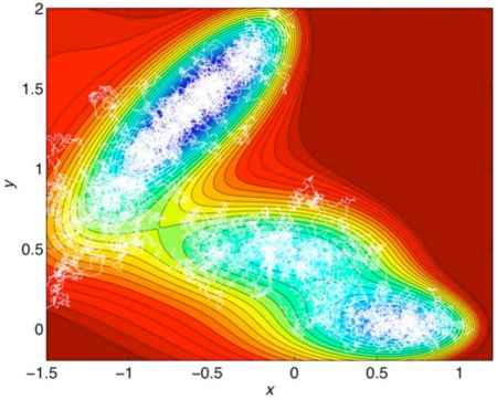
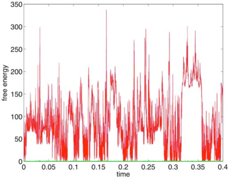
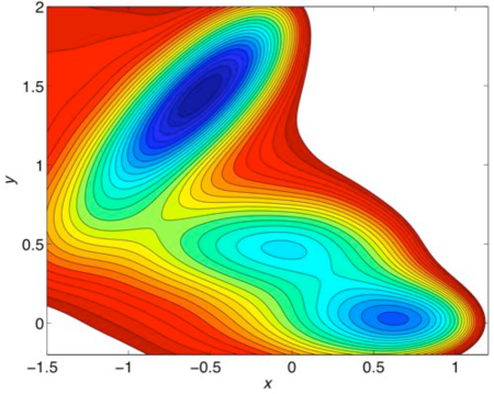
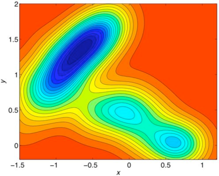
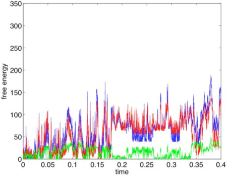
What this entails in terms of efficiency can be illustrated on the two-dimensional Mueller example considered before. In this example, to generate the metadynamics trajectory we used (12) with flooding terms added as in (14), consistent with what was done in Ref. meta3 to test the efficiency of metadynamics in a similar set-up. Fig. 5 shows the metadynamics trajectory obtained by integrating (14) for $2\cdot 10^{4}$ timesteps with a time-step of $\mathit{\Delta}t=2\cdot 10^{-5}$ (same as in the single-sweep method for the results shown in Figs. 1 to 2). As can be seen in Fig. 5, this number of timesteps was enough for the trajectory to visit the important regions of the potential. The reconstructed free energy from this calculation is compared in Fig. 6 to the original one. The metadynamics result is also compared in Fig. 7 to the one obtained by the single-sweep method with $174$ centers. The error (13) for this metadynamics calculation was $e_{1}=0.16$, i.e. almost two orders of magnitude higher than with the single-sweep method. Fig. 8 shows the original and reconstructed Mueller potential along the metadynamics trajectory (blue and red lines, respectively), together with the absolute value of their difference (green line). By comparing Figs. 4 and 8, it can be seen that the discrepancy between the original and reconstructed potential is much larger with metadynamics than with the single-sweep method on trajectories of the same length. Note that these results clearly indicates that it is not sufficient that the metadynamics trajectory visits once a region on phase space to get an accurate representation of the free energy in this region. This was already noted in Refs. lelievre ; meta3 .

Figure 6: Comparison between the level sets of the original Mueller potential (red curves) and the reconstructed potential using metadynamics with a trajectory of $2\cdot 10^{4}$ steps with a time-step of ${\mathit{\Delta}}t=2\cdot 10^{-5}$ (same as in Figs.1 and 3). We only use 10 level sets evenly distributed between $V=0$ and $V=180$ because the differences between the maps are much bigger than with the single-sweep method and drawing more level sets makes the figure difficult to read. (There are only seven black level sets in the energy reconstructed by metadynamics because it levels off around $V=140$.)

Figure 7: Comparison between the Mueller potential as reconstructed by the single-sweep method (upper panel) and metadynamics (lower panel) both with a trajectory of $2\cdot 10^{4}$ steps and a time-step of ${\mathit{\Delta}}t=2\cdot 10^{-5}$. Other representation of these contourplots were already shown in Figs. 3 and 6 respectively. The map reconstructed by the single-sweep method is very close to the map of the original Mueller potential. The colormaps used in both panels are the same and the reconstructed potentials are shifted so that their minimum is $V=0$; the white region in the left panel is where the energy is above $180$ and is not shown (the result of metadynamics shown in the right panel levels off around $V=140$ which is why there is no white).

We were able to improve the metadynamics result by extending the simulation to $2\cdot 10^{5}$ steps. The covering of the important regions in the potential was now extensive (data not shown), and the reconstructed potential (data not shown) looked visually better than the one obtained with the shorter trajectory. Yet the error (13) was $e_{1}=0.12$, i.e. still two orders of magnitude larger than the highest error we obtained with the single-sweep method using a 10 times shorter trajectory. We did not attempt to go to longer runs with metadynamics because the memory term in (14) makes such simulations increasingly expensive (their cost scales as the square of the number of timesteps). It should also be stressed that in all these calculations, we optimized the parameters $\nu$, $\sigma$ and $1/\beta$ the best we could. This optimization, however, turns out to be complicated since there is no systematic way to perform it because, unlike with the single-sweep method, there is no objective function to minimize in metadynamics. The results shown in Figs. 5–8 were obtained with $\nu=2\cdot 10^{3}$, $\sigma=0.2$ and $1/\beta=10$.

To be fair, we should conclude this comparison by mentioning that the simplicity of the Mueller potential example tends to exaggerate the gain that the single sweep method provides over metadynamics. Indeed, in realistic situations, the single-sweep method also requires to compute the mean force via (11), an operation which was unnecessary in the Mueller example since the force was readily available. Computing the mean force adds an extra cost to the method. It is worth stressing again, however, that the computation of the time averages in (11) can be distributed over several processors. This means that in the ideal situation where the user has at least one processor per center, the effective time to compute all of the mean forces is the same as the one for computing a single one of these forces, i.e. we have perfect scalability. Metadynamics can be parallelized per replica as well, as was proposed in Refs. metap1 ; metap2 ; metap3 , but not as straightforwardly and not with perfect scalability. Indeed, in all of these versions of metadynamics, the simulated replica are never completely independent from each other.

Figure 8: Comparison of the original (blue line) and reconstructed Mueller potential (red line) computed along the $2\cdot 10^{4}$ steps metadynamics shown in Fig. 5. The green line shows the absolute value of the difference between the two. The green line here should be compared with the one in Fig. 4 for the single-sweep method: the discrepancy between the original and reconstructed potential is always larger with metadynamics than with the single-sweep method.

V Free energy of alanine dipeptide in solution

In this section, we use the single-sweep method to reconstruct the free energy of the solvated alanine dipeptide (AD) molecule in two and four torsion angles at $300$ K. While AD is not an example of biochemical interest per se, we study it because it has been extensively used as a benchmark example for free energy calculations in the literature karplus ; tuckad ; meta_ad . On top of this the system is simple enough that we can use it to systematically investigate how the accuracy of the reconstruction method depends on the number of centers and how robust the method is with respect to statistical errors in the input data for the mean forces. Another question we investigate in this section is the robustness of the method against the choice of radial-basis functions. Specifically, we compare results obtained using the Gaussian packet (3) and the Wendland function

$$\varphi(u)={(1-u)^{6}_{+}(35u^{2}+18u+3)}$$ (16)

where $(f(u))_{+}=f(u)$ if $f(u)>0$, and $(f(u))_{+}=0$ otherwise. (16) is another well-known example of radial-basis function which has the pleasant property that it is compactly supported. This property is appealing in the calculations since it limits the range over which centers interact in (4).

All MD simulations reported below were performed with a version of the MOIL code moil suitably modified by us, and the AMBER/OPLS ff force field (for details of the MD set-up see Appendix A).

V.1 Two angles calculation

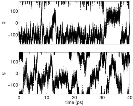
We use the standard dihedral angles $\phi$ and $\psi$. At $300$ K, the system is confined in a region of the $(\phi,\psi)$ space with $\phi<-50^{\circ}$ by energy barriers higher than $1/\beta$. In order to overcome these barriers and sweep through the whole $[-180^{\circ},180^{\circ}]^{2}$ space, we generated a trajectory by using (8) with $(z_{1},z_{2})=(\phi,\psi)$, $\kappa=100$ kcal/mol/rad², a friction coefficient $\gamma=0.5$ kcal$\times$ps/mol/rad² and an artificial temperature $1/\bar{\beta}=9.5$ kcal/mol. With this choice of the parameters, the important regions of the $[-180^{\circ},180^{\circ}]^{2}$ space were visited in $4\cdot 10^{4}$ steps ($40$ ps in the time units of the MD variables). The time series of $\phi$ and $\psi$ along this trajectory are shown in Fig. 9. Variations in $\kappa$, $\gamma$ and $1/\bar{\beta}$ led to qualitatively similar TAMD trajectories, indicating that the the method is robust with regard to the choice of these parameters. Sets with a different number $K$ of centers were deposited along the TAMD trajectory afterwards by processing this trajectory using various distances $d$ between the centers. Specifically, we generated sets of $90$, $128$, $151$, $188$, $219$ and $262$ centers using, respectively, $d=31.77^{\circ}$, $26.00^{\circ}$, $23.87^{\circ}$, $21.37^{\circ}$, $20.00^{\circ}$, $17.92^{\circ}$.

Figure 9: Time series of the dihedral angles $\phi$ and $\psi$ along the $40$ ps long TAMD trajectory for the solvated alanine dipeptide (AD).

Given a set of $K$ centers $(\phi_{k},\psi_{k})$, we computed the mean forces via $K$ independent MD simulations with restraints at $(\phi,\psi)=(\phi_{k},\psi_{k})$, i.e. by simulating (10) in the isokinetic ensemble at $300$ K, and estimated the mean force via (11) with $\bar{\kappa}=100$ kcal/mol/rad². This value of $\bar{\kappa}$ was high enough since we checked that the reconstructed free energy remained invariant with higher values of $\bar{\kappa}$ (we did so up to $\bar{\kappa}=10^{3}$ kcal/mol/rad²). We then used this data in the reconstruction procedure explained in Sec. II.1. Note that since the free energy in the $(\phi,\psi)$ angle is periodic, we have to periodically extend the centers for the representation. This amounts to changing the representation in (2) into

$$\tilde{A}({\bm{z}})=\sum_{\hat{{\bm{n}}}\in Z^{N}}\sum_{k=1}^{K}a_{k}\varphi_{\sigma}(|{\bm{z}}-{\bm{z}}_{k}+2\pi~{}\hat{{\bm{n}}}\cdot\hat{{\bm{e}}}|)+C,$$ (17)

where $\hat{{\bm{e}}}$ is the unit vector in $\mathbb{R}^{N}$. In practice, only few periodic replica of the centers are needed (i.e. $\hat{n}_{i}=2$ for $i=1,\dots,N$) because the radial-basis functions centered at the centers further away from the cell under consideration make negligible contributions to the result in this cell.

V.1.1 Calculation with $d=21.37^{\circ}$ ($188$ centers) and $T=50$ ps.

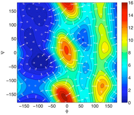
We first detail our result with this choice of parameters to pick an example which led to a good balance between accuracy and efficiency. Other choices of parameters are discussed below. Thus, Fig. 10 shows the reconstructed free energy map obtained with $d=21.37^{\circ}$ ($188$ centers) and by computing the mean forces from (11) with $T=50$ ps. The optimal $\sigma$ in this calculation was $\sigma^{\star}=44.73^{\circ}$. In the figure, the minimum of the free energy is set at $0$ kcal/mol, and contour levels are plotted at $0.5$ kcal/mol, $1$ kcal/mol and then every $1$ kcal/mol. The centers are represented as white circles, and the mean forces at the centers as arrows.

Figure 10: Free energy of AD in the $\phi$ and $\psi$ dihedral angles at $300$ K calculated with the single-sweep method by using $188$ centers deposited at a distance of $d=21.37^{\circ}$ from each other. Units for the free energy are kcal/mol, and contour levels are plotted at $0.5$ kcal/mol, $1$ kcal/mol, and then every $1$ kcal/mol. The optimal $\sigma$ in this reconstruction was $\sigma=44.73^{\circ}$. The centers are represented as white circles. At every center, the corresponding mean force vector is also shown. Mean forces were calculated by using (11) with $\bar{\kappa}=100$ kcal/mol/rad² and $T=50$ ps.

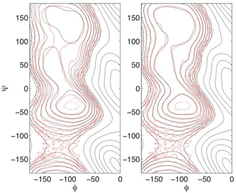
Since the free energy map depends on the force field used, comparison with results in the literature is difficult. To assess the accuracy of our result self-consistently, we compared it with the free energy calculated by computing the PDF of $\phi$ and $\psi$ from a direct MD simulation (DMDS) of about $30$ ns. While this trajectory does not cover all the $[-180^{\circ},180^{\circ}]^{2}$ space, it covers the important regions and allows for an unbiased estimation of the free energy in these regions which can be used as benchmark. The left panel in Fig. 11 shows the contour levels of the free energy from the single-sweep (black lines) and that from DMDS (red lines). The contour levels are plotted at $0.1$ kcal/mol (dotted lines), every $0.5$ kcal/mol from $0.5$ to $4$ kcal/mol, and then every $2$ kcal/mol. As can be seen, single-sweep results agree remarkably well with those of the DMDS.

In terms of cost, to generate the result shown in Fig. 10, we had to make one simulation run of $40$ ps to generate the TAMD trajectory, plus $188$ independent runs of $50$ ps distributed on different nodes (the additional cost of estimating the parameters $a^{\star}_{k}$ and $\sigma^{\star}$ to use in (2) is insignificant). This makes for a total of $9.4$ ns of absolute simulation time. However, after distribution, the effective simulation time needed is only $90$ ps. On top of this, we show below that a good estimate of the free energy can be obtained with as low as 90 centers (i.e. with an absolute simulation time of $4.5$ ns and the same effective simulation time, $90$ ps). For comparison, in Ref. meta_ad Ensing et al. report a $4$ ns calculation performed with metadynamics to estimate the free energy of AD in $\phi$ and $\psi$. It is not clear how well this metadynamics calculation can be parallelized to reduce its effective cost (it was not parallelized in Ref. meta_ad ). In addition, the result of this metadynamics calculation is unlikely to be as accurate as the one in Fig. 10 (in Ref. meta_ad no comparison like the one shown in Fig. 11 is provided)

Figure 11: Comparison between the free energy obtained by single-sweep (black lines) method and DMDS (red lines) for AD. The left panel shows the result with with $188$ centers, the right panel the one with $262$ centers. The contour levels of the free energy are plotted at $0.1$ kcal/mol (dotted lines), from $0.5$ to $4.0$ kcal/mol separated by $0.5$ kcal/mol, and then separated by $2$ kcal/mol.

V.1.2 Robustness and convergence analysis

Next we analyze how robust are the results with respect to the statistical error in the mean force data and the choice of radial-basis function. We also analyze convergence in function of the number of centers. As reference value, we take the free energy reconstructed with $d=17.92^{\circ}$ ($262$ centers) and $T=250$ ps of time averaging in (11). The map of the free energy calculated with these parameters (data not shown) is visually very similar to the one shown in Fig. 10, but it is more accurate. The residual error can be estimated from the right panel of Fig. 11 which shows the contour levels of the free energy from the single-sweep (black lines) and that from DMDS (red lines): these level sets coincide up to statistical errors in the DMDS, indicating that the free energy provided by the single sweep method with $262$ centers and $T=250$ ps can indeed be taken as an “exact” benchmark.

Figure 12: Difference maps with respect to the AD free energy in $\phi$ and $\psi$ reconstructed with Gaussian functions using $262$ centers and $T=250$ ps. The figures in the different panels correspond to various number of centers and length of time averaging for the mean forces, as indicated. Units are kcal/mol. Note that the scale of the colormap is different from the one in Fig. 10. In particular, the differences are mostly below $0.5$ kcal/mol with $151$ centers and $50$ ps simulations already.

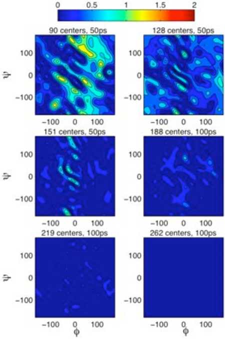
Fig. 12 shows the differences between the map of the reference free energy reconstructed with $d=17.92^{\circ}$ ($262$ centers) and $T=250$ ps and those reconstructed with less centers and shorter restrained simulations. The largest errors are in the regions corresponding to the highest peaks of the free energy (these are also the regions were the least centers were deposited). The differences never exceed $1.25$ kcal/mol with $90$ centers and $T=50$ ps and they fall mostly below $0.5$ kcal/mol with $151$ centers and $T=50$ ps already.

We also compared the quality of the reconstruction of the free energy when using Gaussian (3) and Wendland (16) basis functions. Fig. 13 shows the residual per center versus the number of centers for AD, by using Gaussian (filled symbols) and Wendland (empty symbols) basis functions, using $T=50$ ps (diamonds) and $T=250$ ps (circles) long restrained simulations to estimate the mean forces. At equal values of $K$ and $T$, the reconstruction is slightly more accurate with Gaussian than with Wendland functions, though these differences turn out to be quite small in terms of the free energy maps themseves (data not shown).

Figure 13: Residual per center versus number of centers in the reconstruction of the AD free energy in $\phi$ and $\psi$ angles. Data are from calculations with different time averaging length, using Gaussian (G) and Wendland (W) basis functions.

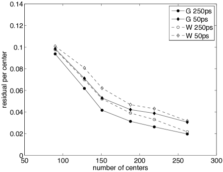
Using longer simulations for the mean force (which means a smaller random error on these forces) also improves the results. With $262$ centers and $T=250$ ps long simulations for the mean forces, the maps reconstructed with Gaussian and Wendland basis functions were almost identical (data not shown), and they were not significantly different from the map shown in Fig. 10. These results, however, were obtained at very different values of optimal $\sigma$: $\sigma^{\star}=26.33^{\circ}$ with Gaussians and $\sigma^{\star}=123.20^{\circ}$ with Wendland functions. The condition numbers at the optimal $\sigma$ were $3889.67$ and $868.86$, respectively, which is low. Note that the same trends here described were observed in a periodic test case for which the potential was known exactly (data not shown).

V.2 Four angles calculation

As a second more challenging test, we computed the free energy of AD in the four torsion angles, $\phi$, $\psi$, $\theta$, and $\zeta$. A TAMD trajectory of $44$ ps was generated by using (8) with $(z_{1},z_{2},z_{3},z_{4})=(\phi,\psi,\theta,\zeta)$, $\kappa=100$ kcal/mol/rad², an artificial temperature $1/\bar{\beta}=9.5$ kcal/mol, friction coefficients $\gamma=0.5$ kcal$\times$ps/mol/rad² for $\phi$ and $\psi$ and $\gamma=1$ kcal$\times$ps/mol/rad² for $\theta$ and $\zeta$. The MD potential keeps the amide planes in trans configuration, and so $\theta$ and $\zeta$ were varying in the range $[-70^{\circ},70^{\circ}]$. In $44$ ps, the TAMD trajectory covered well the accessible state space for $\phi$, $\psi$, $\theta$ and $\zeta$, in the sense that the time series for these angles were similar in their respective state space to those shown in Fig. 9 (notice however that extensive coverage of the four-dimensional space is unlikely in so short a run). Along the TAMD trajectory, $200$ centers at a distance of $d=45.84^{\circ}$ were deposited. At these centers, the mean forces ${\bm{f}}_{k}$ were computed by using (11) with $\bar{\kappa}=100$ kcal/mol/rad² and $T=50$ ps (i.e. the absolute time of simulation was about $10$ ns, but the effective time after distribution was $94$ ps only). We used these ${\bm{f}}_{k}$ in the objective function (4) to finally get the representation (2) of the four-dimensional free energy $\tilde{A}(\phi,\psi,\theta,\zeta)$. The optimal $\sigma$ in this representation was $\sigma^{\star}=67.63^{\circ}$ and the condition number at this value of $\sigma$ was $4214.05$.

Figure 14: Free energy of AD in the $\phi$, $\psi$, $\theta$ angles obtained from the marginal in these angles of the PDF associated with the free energy in four angles $\tilde{A}(\phi,\psi,\theta,\zeta)$. Data are represented for $\theta\in[-50^{\circ},-3^{\circ}]$. Note that the scale of the colormap is different from the one in Fig. 10

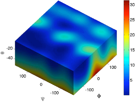
Since a full graphical representation of $\tilde{A}(\phi,\psi,\theta,\zeta)$ is not possible, we did several tests to validate our result. Fig. 14 shows the three dimensional free energy $\tilde{A}(\phi,\psi,\theta)$ obtained from the marginal in these angles of the PDF associated with $\tilde{A}(\phi,\psi,\theta,\zeta)$. This marginal was calculated a posteriori by numerical integration over $\zeta$ of $e^{-\beta\tilde{A}(\phi,\psi,\theta,\zeta)}$ with the full $\tilde{A}(\phi,\psi,\theta,\zeta)$ reconstructed by the single-sweep method. The map is reasonable, and shows nontrivial features in all three directions. Fig. 15 shows the two dimensional free energy $\tilde{A}(\phi,\psi)$ obtained from the marginal in these angles of the PDF associated with $\tilde{A}(\phi,\psi,\theta,\zeta)$. The map is in remarkably good agreement with the one in Fig. 10.

As a further test of accuracy, we re-calculated the mean force using (10) and (11) using a different set of centers than those used in (2). Then we estimated the relative error between these mean forces and the ones obtained by taking the negative gradient of the reconstructed $\tilde{A}(\phi,\psi,\theta,\zeta)$ using the original set of centers and mean forces:

$$\varepsilon_{k}=\frac{|\nabla_{\!z}\tilde{A}({\bm{z}}^{n}_{k})+{\bm{f}}^{n}_{\!k}|}{|{\bm{f}}^{n}_{\!k}|}$$ (18)

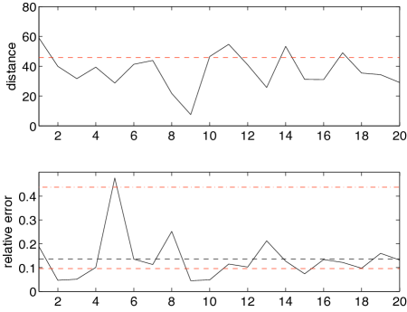
where ${\bm{z}}^{n}_{k}$ are the new centers and ${\bm{f}}^{n}_{\!k}$ are the mean forces at these centers. The new centers were 20 points chosen at random in the domains $\phi,\psi\in[-180^{\circ},180^{\circ}]$, $\theta,\zeta\in[-70^{\circ},70^{\circ}]$.

Figure 15: Free energy of AD in the $\phi$, $\psi$ angles obtained from the marginal in these angles of the probability density associated with the free energy in four angles $\tilde{A}(\phi,\psi,\theta,\zeta)$. Contour levels are as in Fig. 10. Note the remarkable agreement between this map and the one shown in Fig. 10.

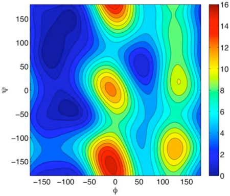
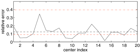
Fig. 16, top panel, shows, for each of these centers, the distance from the closest of the $200$ centers (black line). Data are compared to the minimal distance between the $200$ centers (red dashed line). This result shows that, with $d=45.84^{\circ}$, these centers fill properly the four dimensional domain in the sense that every new center is always a distance about $d$ to one of the original centers. Fig. 16, middle panel, shows the relative error $\varepsilon_{k}$ for $k=1,\dots,20$ (black solid line), when $T=50$ ps long restrained simulations are used to compute the mean forces. The mean value of $\varepsilon_{k}$ (black dashed line) is $0.14$, with standard deviation $0.09$ and maximum value $0.47$. For comparison, the mean value of the relative residual per center (red dashed line) is $0.09$, with standard deviation $0.06$ and maximum value $0.44$ (red dashed-dotted line). Fig. 16, bottom panel, shows $\varepsilon_{k}$ when $T=250$ ps long restrained simulations are used to compute the mean forces. In this case, the mean value of $\varepsilon_{k}$ (black dashed line) is $0.12$, with standard deviation $0.07$ and its maximum value is $0.34$. For comparison, the mean value of the relative residual per center (red dashed line) is $0.09$, with standard deviation $0.06$ and maximum value $0.39$ (red dashed-dotted line).

These results show that, in points away from the original centers, the reconstructed free energy is as accurate as it is at the centers, which is clearly the best we can hope for.

Figure 16: Accuracy of the reconstruction of the free energy of AD in four angles. Top panel, distance of each of the random centers from the closest of the $200$ centers (black line), compared with the minimal distance between the $200$ centers (red line). Middle and lower panel, relative error $\varepsilon_{k}$ defined in (18) for mean forces computed respectively from $50$ and $250$ ps restrained simulations: the error $\varepsilon_{k}$ (black solid line) and its mean value (black dashed line), compared with the mean value of the relative residual per center for the $200$ centers set (red dashed line) and its maximum value (red dashed-dotted line).

VI Concluding remarks

In summary, we have proposed a method for the calculation of free energies which is simple, accurate, and efficient. Unlike standard histogram methods such as WHAM and metadynamics, the single-sweep method uses the mean force computed at a set of centers to reconstruct the free energy. This set of centers is determined using TAMD to rapidly sweep through the important regions of the free energy, and the mean forces at these centers are estimated in a standard way via the computation of a conditional expectation using time-averaging along restrained or constrained simulations. From these data, the free energy $A({\bm{z}})$ is then reconstructed globally by minimization of an objective function to determine the coefficients in a radial-basis function representation of $A({\bm{z}})$. If convenient, this reconstruction step can use data for the centers and the mean forces obtained by other means than TAMD.

Compared with histogram methods and metadynamics, the single-sweep technique combines several advantages:

• It does not require a priori knowledge of the free energy since it uses TAMD to find the important regions in the landscape automatically.

• The most costly step of the calculation, namely the computation of the mean forces at the centers, can be straightforwardly distributed on different, independent, processors.

• The reconstruction step is variational, i.e. the optimal coefficients in the free energy representation are determined automatically, which limits the number of parameters to adjust beforehand.

• The results can be easily monitored for convergence, and systematically improved if desired. In particular, new centers can be added on top of previous ones along the same TAMD trajectory to increase the accuracy without having to repeat the previous calculation.

• The method can be used in more than 2 dimensions and its computational complexity is the same regardless of the dimension.

We believe that these features make the single-sweep method appealing to calculate the free energy of systems more complicated but also more interesting than the ones studied in this paper.

Appendix A Details of the MD simulations

All MD simulations were performed with the MOIL code moil , and the AMBER/OPLS ff force field as implemented in the code. A starting structure for the AD molecule (CH₃-CO-NH-C_αHCH₃-CO-NH-CH₃) was solvated in a box of $252$ water molecules of volume $(20~{}\text{\AA})^{3}$. Periodic boundary conditions were used. Van der Waals interactions were truncated at $9$ Å. Electrostatic interactions were treated with the Particle Mesh Ewald method spme with real space cutoff $9$ Å, a grid of $32^{3}$ points, and $4$-th order B-splines for the interpolation of the structure factor (in order to be in the high accuracy range spme ). The TIP3 model tip3 was used for the water molecules. Non-bonded interaction lists were updated every $10$ steps. All chemical bonds in the system were kept fixed with the SHAKE algorithm shake . Amide planes were restrained to be always in trans configuration. The Velocity Verlet algorithm was used for the dynamics of the Cartesian variables with time-step $1$ fs, and all velocities were scaled at every step to keep the temperature at $300$ K. In order to obtain the initial configuration for the temperature accelerated MD simulation (TAMD), the system was first equilibrated for $100$ ps by keeping the solute molecule fixed (i.e. by zeroing forces and velocities of its atoms) and by assigning to all water atoms at every step velocities sampled from a Maxwell distribution at $300$ K. Then, the whole system was simulated for $400$ ps for equilibration. The torsion angles used in the simulations are defined by the quadruplets of atoms (C,N,C_α,C) and (N,C_α,C,N) for $\phi$ and $\psi$, and (O,C,N,C_α) and (C_α,C,N,H) for $\theta$ and $\zeta$. In the TAMD simulation, the equations of motion of the collective variables were integrated with the forward Euler scheme with time-step $1$ fs, $\gamma=0.5$ kcal$\times$ps/mol/rad² for $\phi$ and $\psi$ and $\gamma=1$ kcal$\times$ps/mol/rad² for $\theta$ and $\zeta$. The force constant for the restraint potential was $\kappa=100$ kcal/mol/rad², and the effective temperature such that $\bar{\beta}^{-1}=9.5$ kcal/mol. The Cartesian coordinates of water and AD atoms were saved during the TAMD simulation. In this way, for every center ${\bm{z}}_{k}$ deposited along the trajectory in collective variables space, there is a corresponding configuration ${\bm{x}}_{k}$ of the system in Cartesian space such that $\theta({\bm{x}}_{k})\approx{\bm{z}}_{k}$. We used these configurations as initial conditions for the restrained simulations at the centers. Data for the mean force calculations were accumulated after further relaxation of the system for $5$ ps.

References

- (1) E. M. Boczko and C. L. Brooks 3rd, Science. 269, 393 (1995).
- (2) T. Simonson, G. Archontis, and M. Karplus, Acc. Chem. Res. 35, 430 (2002).
- (3) J. D. Faraldo-Gómez and B. Roux, Proc. Natl. Acad. Sci. U.S.A. 104, 13643 (2007).
- (4) S. Kumar, J. M. Rosenberg, D. Bouzida, R. H. Swendsen, and P.A. Kollman, J. Comput. Chem. 13, 1011 (1992).
- (5) G. M. Torrie and J. P. Valleau, Chem. Phys. Lett. 28, 578 (1974).
- (6) C. Bartels and M. Karplus, J. Comput. Chem. 18, 1450 (1997).
- (7) A. Laio and M. Parrinello, Proc. Natl. Acad. Sci. U.S.A. 99. 12562 (2002).
- (8) A. Iannuzzi, A. Laio, and M. Parrinello, Phys. Rev. Lett. 90, 238302 (2003).
- (9) E. A. Carter, G. Ciccotti, J. T. Hynes, and R. Kapral, Chem. Phys. Lett. 156, 472 (1989).
- (10) J. G. Kirkwood, J. Chem. Phys. 3, 300 (1935).
- (11) L. Maragliano and E. Vanden-Eijnden, Chem. Phys. Lett. 426, 168 (2006).
- (12) J. VandeVondele and U. Rothlisberger, J. Phys. Chem. B. 106, 203 (2002).
- (13) L. Rosso, P. Mináry, Z. Zhu, and M. E. Tuckerman, J. Chem. Phys. 116, 4389 (2002).
- (14) I. Foster and C. Kesselman, The Grid 2: Blueprint for a New Computing Infrastructure. (Morgan Kaufmann, 2003).
- (15) F. Berman, G. Fox, A. J. G. Hey (Eds.), Grid Computing: Making The Global Infrastructure a Reality. (John Wiley & Sons, 2003)
- (16) R. Schaback, Adv. Comp. Math. 3, 251 (1995).
- (17) M. D. Buhmann, Acta. Numer. 9, 1 (2000).
- (18) P. Niyogi and F. Girosi, Adv. Comp. Math. 10, 51 (1999).
- (19) H.-J. Bungartz H-J and M. Griebel, Acta. Numer. 13, 1 (2004).
- (20) G. Ciccotti, R. Kapral, and E. Vanden-Eijnden, Chem. Phys. Chem. 6, 1809 (2005).
- (21) G. Ciccotti, T. Lelièvre, and E. Vanden-Eijnden, Comm. Pure. App. Math. to appear (available from “early view”).
- (22) K. Mueller, Angew. Chem. 19, 1 (1980).
- (23) A term is typically added to (14) and the thermostat can be different, but this is not essential for our discussion and does not change our conclusions.
- (24) T. Lelièvre, M. Rousset, G. Stoltz, J. Chem. Phys. 126, 134111 (2007).
- (25) G. Bussi, A. Laio, and M. Parrinello, Phys. Rev. Lett. 96, 090601 (2006).
- (26) P. Raiteri, A. Laio, F. L. Gervasio, C. Micheletti, and M. Parrinello, M. J. Phys. Chem. B. 110, 3533 (2005).
- (27) G. Bussi, F. L. Gervasio, A. Laio, and M. Parrinello, J. Am. Chem. Soc. 128, 13435 (2006).
- (28) S. Piana and A. Laio, J. Phys. Chem. B. 111, 4553 (2007).
- (29) L. Rosso, J. B. Abrams, and M. E. Tuckerman, J. Phys. Chem. B, 109, 4162 (2005).
- (30) B. Ensing, M. De Vivo, Z. Liu, P. Moore, and M. L. Klein, Acc. Chem. Res. 39, 73 (2006).
- (31) R. Elber, A. Roitberg, C. Simmerling, R. Goldstein, H. Li, G. Verkhivker, C. Keasar, J. Zhang, and A. Ulitsky, Comp. Phys. Comm. 91, 159 (1995).
- (32) W. L. Jorgensen and J. Tirado-Rives, J. Am. Chem. Soc. 110, 1657 (1998).
- (33) U. Essmann, L. Perera, M. L. Berkowitz, T. Darden, H. Lee, and L. G. Pedersen, J. Chem. Phys. 103, 8577 (1995).
- (34) W. L. Jorgensen, J. Chandrasekhar, J. D. Madura, R. W. Impey, and M. L. Klein, J. Chem. Phys. 79, 926 (1983).
- (35) J. P. Ryckaert, G. Ciccotti, H. J. C. Berendsen, J. Comput. Phys. 23, 327 (1977).