Orbital Optimization in the Density Matrix Renormalization Group, with applications to polyenes and $\beta$-carotene

Abstract

In previous work we have shown that the Density Matrix Renormalization Group (DMRG) enables near-exact calculations in active spaces much larger than are possible with traditional Complete Active Space algorithms. Here, we implement orbital optimisation with the Density Matrix Renormalization Group to further allow the self-consistent improvement of the active orbitals, as is done in the Complete Active Space Self-Consistent Field (CASSCF) method. We use our resulting DMRG-CASSCF method to study the low-lying excited states of the all-trans polyenes up to $\text{C}_{24}\text{H}_{26}$ as well as $\beta$-carotene, correlating with near-exact accuracy the optimised complete $\pi$-valence space with up to 24 active electrons and orbitals, and analyse our results in the light of the recent discovery from Resonance Raman experiments of new optically dark states in the spectrum.

I Introduction

The Density Matrix Renormalization Group (DMRG) is an electronic structure method that has recently been applied to ab-initio quantum chemistry. The method originated in the condensed matter community with the pioneering work of White White1992 ; White1993 . Although the earliest quantum chemistry implementations are only a few years old, the DMRG has already enabled the solution of many problems that would be intractable with any other method White1999 ; Mitrushenkov2001 ; Chan2002 ; Legeza2003dyn ; Moritz2007 . For example, we have shown that the DMRG can obtain near-exact solutions to multireference problems with active spaces much larger than are possible with traditional active space techniques. Such problems have ranged from molecular potential energy curves Chan2003 ; Chan2004b , to the ground and excited states of large conjugated polymers Hachmann2006 ; Dorando2007 ; Hachmann2007 , to metal-insulator transitions in hydrogen chains Hachmann2006 . In each of these cases, we obtained DMRG energies within $0.001$-$0.1$m$E_{h}$ of the (estimated) exact Full Configuration Interaction (FCI) energies in the active space, but for active spaces that, in some problems, have been as large as 100 active electrons in 100 orbitals Hachmann2006 . The development of the DMRG in quantum chemistry has proceeded through the efforts of several groups, and we mention here the work of White et al. White1999 ; Daul2000 ; Rissler2006 , Mitrushenkov et al. Mitrushenkov2001 ; Mitrushenkov2003 ; Mitrushenkov2003nort , our contributions Chan2002 ; Chan2003 ; Chan2004 ; Chan2004b ; Chan2005 ; Hachmann2006 ; Dorando2007 ; Hachmann2007 , the work of Legeza, Hess et al. Legeza2003dyn ; Legeza2003qie ; Legeza2003lif ; Legeza2004 , the work of Reiher et al. Moritz2005orb ; Moritz2005rel ; Moritz2006 ; Moritz2007 , and most recently the work of Zgid and Nooijen Zgid2008 . Also related, but too numerous to cite in full here, are earlier developments of the method for semi-empirical Hamiltonians; some representative contributions are those in Refs. Ramasesha1997 ; Yaron1998 ; Shuai1998 ; Fano1998 ; Bendazzoli1999 ; Raghu2002a ; Raghu2002b .

At the heart of the DMRG is a wavefunction ansatz and the DMRG “algorithm” is simply an efficient variational optimisation procedure for this ansatz. Unlike most wavefunctions in quantum chemistry, the DMRG wavefunction is not parametrised by excitations from an underlying reference state. Rather, it is built directly from local variational objects (which we shall later call site functions) which are associated with the active orbitals in the system, and which describe how the orbitals are correlated with each other. Each site function is characterised by a rank $M$ that measures the number of variational parameters, and as this rank increases the ansatz becomes exact. For an incomplete rank $M$, correlations between orbitals that are widely separated in the ansatz are truncated. Thus the DMRG is a naturally local theory, but, since the ansatz is not constructed from a reference, it is a local multireference theory. This may be seen as the basic reason why the DMRG can describe very large multireference problems so easily. We should note that the structure of the DMRG wavefunction means that it is a local theory only in the number of correlating orbitals along one of the physical dimensions of the problem. However, generalisations of the ansatz to a local theory along all physical dimensions are now known, and are under active development Verstraete2004pbc ; Verstraete2004peps ; Perez-Garcia2007 ; Schuch2007 ; Murg2007 ; Vidal2006 .

In most applications of the DMRG to quantum chemistry so far, the active space of interest has been easy to identify, i.e. there is a good core-valence and valence-Rydberg separation, either for energetic or symmetry reasons, allowing the DMRG to be used with such an active space as a direct substitute for Complete Active Space Configuration Interaction (CASCI). In general, however, we cannot always identify the active orbitals in a simple way, and thus there is a need for an orbital optimised DMRG, where the active space is determined self-consistently by energy minimisation, in much the same way as in the Complete Active Space Self-Consistent Field (CASSCF) method Roos1986 ; Roos1987 . The purpose of the current work is to describe how this may be done. The resulting orbital optimised DMRG we shall refer to as the DMRG-CASSCF method.

While the general idea of orbital optimisation is straightforward, in practice an efficient implementation must be tailored to the underlying many-body wavefunction ansatz. In Sec. II we describe such an algorithm for the DMRG wavefunction. We start with an overview of orbital optimisation in Sec. II.1 that recalls how the procedure may naturally be divided into two tasks, the evaluation of the one- and two-particle density matrices, and the orbital rotation and integral transformation steps. In Sec. II.2 we present an efficient method to evaluate the one- and two-particle density matrices in the DMRG. Our current implementation benefits from the observation of Zgid and Nooijen that the one-site DMRG algorithm is more suitable than the two-site DMRG algorithm for this purpose. To facilitate the large-scale calculations for our applications to long polyenes and $\beta$-carotene in this work, we have fully parallelised not only the evaluation of the reduced density matrices in the DMRG, but also the orbital rotation and integral transformation steps. These implementation aspects are discussed in Sec. II.3. Finally, the complete DMRG-CASSCF macroiteration is summarised in Sec. II.4.

In Sec. III we apply the DMRG-CASSCF method to the problem of the low-lying excitations in polyenes and $\beta$-carotene. The conjugated $\pi$-system in the polyenes and substituted species such as $\beta$-carotene gives rise to an unusual excitation spectrum, with “dark” electronic states lying beneath the optically allowed HOMO-LUMO transition. The electronic structure of these low-lying states lies at the heart of energy transport in systems ranging from conjugated organic semiconductors to the biological centres of light-harvesting and vision. While the relevant active space on these systems clearly consists of the conjugated $\pi$-valence orbitals, to the best of our knowledge previous calculations on these systems have not correlated complete $\pi$-valence spaces with more than 5 double bonds (corresponding to a (10,10) complete active space hirao ; kurashige ). In the current study we use our DMRG-CASSCF method to perform calculations correlating the complete $\pi$-valence space in polyenes up to $\text{C}_{24}\text{H}_{26}$ (with 12 conjugated bonds) and $\beta$-carotene (with 11 conjugated bonds), and analyse our results in relation to recent Resonance Raman measurements, which have detected previously unidentified “dark” states in the low-lying spectrum.

II Theory

II.1 Overview of orbital optimisation

We begin with some general remarks on orbital optimisation in ab-initio quantum chemistry. Starting from the electronic Hamiltonian, specified by the one- and two-electron integral matrix elements $t_{ij}$ and $v_{ijkl}$

$$H=\sum_{ij}t_{ij}a^{\dagger}_{i}a_{j}+\sum_{ijkl}v_{ijkl}a^{\dagger}_{i}a^{\dagger}_{j}a_{k}a_{l}$$ (1)

an ab-initio quantum chemical method provides a wavefunction $\Psi$ that approximates a target eigenstate of $H$. From $\Psi$ we define the one- and two-particle density matrix elements $\gamma_{ij},\gamma_{ijkl}$

$$\gamma_{ij} =\langle\Psi|a^{\dagger}_{i}a_{j}|\Psi\rangle$$ (2)

$$\gamma_{ijkl} =\langle\Psi|a^{\dagger}_{i}a^{\dagger}_{j}a_{k}a_{l}|\Psi\rangle$$ (3)

and the energy expectation value $\langle\Psi|H|\Psi\rangle$ can be written as

$$E=\sum_{ij}t_{ij}\gamma_{ij}+\sum_{ijkl}v_{ijkl}\gamma_{ijkl}$$ (4)

Orbital rotation corresponds to a unitary transformation of the wavefunction effected by an operator $e^{A}$, where $A$ has the single-particle operator form

$$A=\sum_{ij}A_{ij}a^{\dagger}_{i}a_{j}$$ (5)

and $A_{ij}=-A_{ji}^{*}$. After orbital rotation, the transformed wavefunction $\bar{\Psi}$ and energy $\bar{E}$ are

$$\bar{\Psi} =e^{A}\Psi$$

$$\bar{E} =\langle\Psi e^{-A}|H|e^{A}\Psi\rangle$$ (6)

But one can also consider the unitary operator to act on the Hamiltonian rather than the wavefunction, and from this equivalent point of view, we have a transformed $\bar{H}$ and energy expression

$$\bar{H} =e^{-A}He^{A}$$

$$\bar{E} =\langle\Psi|\bar{H}|\Psi\rangle$$ (7)

The transformed Hamiltonian $\bar{H}$ has the same form as the original Hamiltonian (1) but with modified integrals $\bar{t}_{ij}$ and $\bar{v}_{ijkl}$ that reflect the rotated orbitals

$$\bar{t}_{ij} =\sum_{i^{\prime}j^{\prime}}U_{ii^{\prime}}^{*}U_{jj^{\prime}}{t}_{i^{\prime}j^{\prime}}$$

$$\bar{v}_{ijkl} =\sum_{i^{\prime}j^{\prime}k^{\prime}l^{\prime}}U_{ii^{\prime}}^{*}U_{jj^{\prime}}^{*}U_{kk^{\prime}}U_{ll^{\prime}}{v}_{i^{\prime}j^{\prime}k^{\prime}l^{\prime}}$$ (8)

where $U$ is the coefficient matrix $e^{A}$. Thus we can rewrite the energy after orbital rotation in terms of the original one- and two-particle density matrices and the modified integrals

$$\bar{E}=\sum_{ij}\bar{t}_{ij}\gamma_{ij}+\sum_{ijkl}\bar{v}_{ijkl}\gamma_{ijkl}$$ (9)

We include this elementary discussion because it leads directly to the following familar procedure to optimise the orbitals in an ab-initio wavefunction:

1. From the ab-initio method obtain $\Psi$ corresponding to the given $H$ and form the density matrices $\gamma_{ij},\gamma_{ijkl}$.

2. Determine an orbital rotation step $e^{A}$, and form the new Hamiltonian $\bar{H}=e^{-A}He^{A}$ from the transformed integrals.

3. Goto 1. and loop until convergence in $\Psi$.

Note that in the above, the orbital degrees of freedom and the other ansatz degrees of freedom in $\Psi$ are alternately optimised in steps (1), (2). While more sophisticated approaches which couple orbital rotations with changes in the other ansatz degrees of freedom can be envisaged (as are employed in multi-configurational self-consistent field methods knowles ; yeager1982nra ), we shall adopt the above simple strategy to optimise the orbitals in the DMRG wavefunction. The conceptual task is then twofold. Firstly, how do we calculate the one- and two-particle density matrices in the DMRG? And secondly, what method should we use to select our orbital rotation steps and to construct the transformed Hamiltonian?

II.2 Evaluation of the one- and two-particle density matrices in the DMRG

While the algorithm to calculate the one- and two-particle density matrices could, in principle, be described entirely in the traditional Renormalization Group language of the DMRG, we believe that it is beneficial to understand the method in a more modern language which focuses on the structure of the DMRG wavefunction. Thus we begin with a brief review of the general properties of the DMRG wavefunction before proceeding to the method of reduced density matrix evaluation. For an expanded introduction to the wavefunction perspective in DMRG, we refer the reader to our introductory article Ref. Chan-bookchapter as well as other recent reviews in the field SCHOLLWOCK:2005:_dmrg .

II.2.1 The DMRG wavefunction

The DMRG algorithm corresponds to a variational minimisation of the energy within the space of a wavefunction ansatz. To specify this ansatz we first define an ordering of the orbitals thereby mapping them onto sites on a one-dimensional lattice. Then, the “one-site” DMRG ansatz is given by

$$|\Psi_{\text{DMRG}}\rangle=\mathop{\sum_{n_{1}n_{2}n_{3}\ldots n_{k}}}_{i_{1}i_{2}i_{3}\ldots i_{k-1}}\psi^{n_{1}}_{i_{1}}\psi^{n_{2}}_{i_{1}i_{2}}\psi^{n_{3}}_{i_{2}i_{3}}\ldots\psi^{n_{k}}_{i_{k-1}}|n_{1}n_{2}n_{3}\ldots n_{k}\rangle$$ (10)

where $|n_{1}\ldots n_{k}\rangle$ denotes a Slater determinant in occupation number form, i.e. $n_{i}$ is the occupation of orbital $i$, and the total number of orbitals is $k$. The $\psi$ “site functions” are 3-index quantities and are the variational parameters of the wavefunction. The dimension of each $n_{1}\ldots n_{k}$ index is 4, corresponding to the 4 occupancies for each orbital $|-\rangle,|\phi^{\alpha}\rangle,|\phi^{\beta}\rangle,|\phi^{\alpha}\phi^{\beta}\rangle$, while the dimension of each auxiliary index $i_{1}\ldots i_{k-1}$ is some specified size $M$, thus making each site function a tensor of dimension $4\times M\times M$, except for the first and last, which only have two indices and are of dimension $4\times M$. As $M$ increases, the wavefunction ansatz becomes increasingly exact. If we interpret a site function with indices $n_{p},i_{p-1},i_{p}$ as a matrix array $\bm{\psi}^{n_{p}}$ where $i_{p-1},i_{p}$ are the matrix indices and $n_{p}$ is the third, array, index, then the ansatz is written compactly as a matrix product state

$$|\Psi_{\text{DMRG}}\rangle=\mathop{\sum_{n_{1}n_{2}n_{3}\ldots n_{k}}}\bm{\psi}^{n_{1}}\bm{\psi}^{n_{2}}\bm{\psi}^{n_{3}}\ldots\bm{\psi}^{n_{k}}|n_{1}n_{2}n_{3}\ldots n_{k}\rangle$$ (11)

Because of this matrix product structure, the DMRG ansatz is also known as the matrix product state (MPS) Fannes1992 ; Ostlund1995 ; Rommer1997 .

Now the above form of the DMRG ansatz is invariant to transformations of the site functions of the form ($\bm{\psi}^{n_{p}}\to\bm{\psi}^{n_{p}}\mathbf{U}$, $\bm{\psi}^{n_{p+1}}\to\mathbf{U^{\dagger}}\bm{\psi}^{n_{p+1}}$) and thus it is useful to define a canonical form of the DMRG wavefunction that eliminates this freedom. In practice, this canonical representation is used in all DMRG calculations, and it is also the representation in which the link between the DMRG wavefunction and the traditional Renormalization Group language is most direct. In essence, the canonical form of the wavefunction at a given site corresponds to the familiar expression for the DMRG wavefunction where it is expanded in the product basis of the left and right blocks separated by the site White1999 ; Chan-bookchapter .

To obtain the canonical form, we choose a specific site, say $p$, around which to canonicalise. Then the site $p$ canonical form is given as

$$|\Psi\rangle =\sum_{n_{1}\ldots n_{p}\ldots n_{k}}{\bm{L}}^{n_{1}}\ldots{\bm{L}}^{n_{p-1}}{\bm{C}}^{n_{p}}{\bm{R}}^{n_{p+1}}\ldots{\bm{R}}^{n_{k}}|n_{1}\ldots n_{p}\ldots n_{k}\rangle$$ (12)

We label the site functions to the left of $p$ by $L$, and those to the right by $R$. The degeneracy (invariance to transformation) of the original ansatz (10) mentioned above is lifted by requiring the $L$ and $R$ site functions to be orthogonal projection matrices in the following sense

$$\sum_{ln_{q}}L^{n_{q}}_{ll^{\prime}}L^{n_{q}}_{ll^{\prime\prime}} =\delta_{l^{\prime}l^{\prime\prime}}$$ (13)

$$\sum_{rn_{q}}R^{n_{q}}_{r^{\prime}r}R^{n_{q}}_{r^{\prime\prime}r} =\delta_{r^{\prime}r^{\prime\prime}}$$ (14)

i.e. by grouping together the $ln_{q}$ indices to form the row index of a $4M\times M$ matrix, each $L$ site function is orthogonal with respect to its $M$ columns, while by grouping together the $rn_{q}$ indices to form the column index of a $M\times 4M$ matrix, each $R$ site function is orthogonal with respect to its $M$ rows.

The link between the canonical form and the original RG formulation appears when we combine the $L$ site functions $\bm{L}^{n_{1}}\ldots\bm{L}^{n_{p-1}}$ with the basis states $|n_{1}\ldots n_{p-1}\rangle$, and the $R$ site functions $\bm{R}^{n_{p+1}}\ldots\bm{R}^{n_{k}}$ with the basis states $|n_{p+1}\ldots n_{k}\rangle$, to define renormalised left and right many body spaces $\{l_{p-1}\}$, $\{r_{p+1}\}$

$$|l_{p-1}\rangle =\mathop{\sum_{n_{1}\ldots n_{p-1}}}_{l_{1}\ldots l_{p-2}}L^{n_{1}}_{l_{1}}\ldots L^{n_{p-1}}_{l_{p-2}l_{p-1}}|n_{1}\ldots n_{p-1}\rangle$$ (15)

$$|r_{p+1}\rangle =\mathop{\sum_{n_{p+1}\ldots n_{k}}}_{r_{p+2}\ldots r_{k}}R^{n_{p+1}}_{r_{p+1}r_{p+2}}\ldots R^{n_{k}}_{r_{k}}|n_{p+1}\ldots n_{k}\rangle$$ (16)

Since the dimension of the left basis in Eq. (15) is $M$ (i.e. the dimension of the auxiliary index $l_{p-1}$) and similarly for the right basis, the site functions $\bm{L}^{n_{1}}\ldots\bm{L}^{n_{p-1}}$ and $\bm{R}^{n_{p+1}}\ldots\bm{R}^{n_{k}}$ define a projective transformation or renormalization from the many-body spaces $\{n_{1}\}\otimes\ldots\otimes\{n_{p-1}\}$ and $\{n_{p+1}\}\otimes\ldots\otimes\{n_{k}\}$ to the left and right spaces, $\{l_{p-1}\},\{r_{p+1}\}$, respectively. Then, in the renormalised representation, $C^{n_{p}}_{l_{p-1}r_{p}}$ gives the coefficients of expansion of the wavefunction $|\Psi\rangle$, i.e.

$$|\Psi\rangle=\sum_{l_{p-1}n_{p}r_{p}}C^{n_{p}}_{l_{p-1}r_{p}}|l_{p-1}n_{p}r_{p}\rangle$$ (17)

This is just the RG expression for the one-site DMRG wavefunction, in the product space of a renormalised left “block”, a site $p$, and a renormalised right “block”. Thus in the usual DMRG language, the site $p$ canonical form corresponds to the DMRG wavefunction in the basis associated with the block configuration $\framebox{$\bullet_{1}\ldots\bullet_{p-1}$}\ \bullet_{p}\ \framebox{$\bullet_{p+1}\ldots\bullet_{k}$}$.

A one-site DMRG wavefunction expressed in the canonical form of a given site $p$ can always be expressed in the canonical form for any other site (or using the traditional DMRG language, the DMRG wavefunction for a given one-site block configuration can always be expressed in the basis of any other one-site block configuration along a sweep). Since we are simply re-expressing the same wavefunction in a different basis, the coefficients $C$ and site-functions $L,R$ at different sites are related. To see the link explicitly, we compare the canonical forms at adjacent sites $p$, $p+1$

$$|\Psi\rangle =\sum_{n_{1}\ldots n_{p}\ldots n_{k}}{\bm{L}}^{n_{1}}\ldots\bm{L}^{n_{p-1}}\bm{C}^{n_{p}}\bm{R}^{n_{p+1}}\bm{R}^{n_{p+2}}\ldots\bm{R}^{n_{k}}|n_{1}\ldots n_{p}\ldots n_{k}\rangle$$ (18)

$$=\sum_{n_{1}\ldots n_{p}\ldots n_{k}}\bm{L}^{n_{1}}\ldots\bm{L}^{n_{p-1}}\bm{L}^{n_{p}}\bm{C}^{n_{p+1}}\bm{R}^{n_{p+2}}\ldots\bm{R}^{n_{k}}|n_{1}\ldots n_{p}\ldots n_{k}\rangle.$$ (19)

which yields the relation

$$\bm{L}^{n_{p}}\bm{C}^{n_{p+1}}=\bm{C}^{n_{p}}\bm{R}^{n_{p+1}}$$ (20)

Now say we are given $\bm{C}^{n_{p}}\bm{R}^{n_{p+1}}$ from the site $p$ canonical form, and we wish to determine $\bm{L}^{n_{p}}\bm{C}^{n_{p+1}}$ for the site $p+1$ canonical form, where $\bm{L}^{n_{p}}$ satisfies the orthogonality conditions (13). We can obtain such a $\bm{L}^{n_{p}}$ solution of (20) together with $\bm{C}^{n_{p+1}}$ from the singular value decomposition (SVD) of $\bm{C}^{n_{p}}$, viewed as the $4M\times M$ matrix with row indices $l_{p-1}n_{p}$, column indices $r_{p+1}$ and $M$ singular values $\sigma_{l_{p}}$,

$$C^{n_{p}}_{l_{p-1},r_{p+1}} =\sum_{l_{p}}L^{n_{p}}_{l_{p-1},l_{p}}\sigma_{l_{p}}V_{l_{p}r_{p+1}},$$ (21)

$$C^{n_{p+1}}_{l_{p},r_{p+2}} =\sum_{r_{p+1}}\sigma_{l_{p}}V_{l_{p}r_{p+1}}R^{n_{p+1}}_{r_{p+1},r_{p+2}}$$ (22)

The above transformation between canonical forms at adjacent sites corresponds directly to the transformation between block configurations during the sweep algorithm in the DMRG. In particular, Eq. (21) corresponds to the determination of the basis of the renormalised block $\framebox{$\bullet_{1}\ldots\bullet_{p+1}$}$ from the density matrix eigenvectors of the superblock $\framebox{$\bullet_{1}\ldots\bullet_{p}$}\ \bullet_{p+1}$, while Eq. (22) corresponds to the wavefunction transformation used to generate the guess at a given block configuration from that at the previous configuration. We note in passing that an exact transformation between canonical forms at different sites is only possible with the one-site DMRG ansatz. Most DMRG calculations use the two-site DMRG ansatz with the block configuration $\framebox{$\bullet_{1}\ldots\bullet_{p-1}$}\ \bullet_{p}\bullet_{p+1}\ \framebox{$\bullet_{p+2}\ldots\bullet_{k}$}$ and a corresponding canonical form at site $p$

$$|\Psi\rangle =\sum_{n_{1}\ldots n_{p}\ldots n_{k}}{\bm{L}}^{n_{1}}\ldots{\bm{L}}^{n_{p-1}}{\bm{C}}^{n_{p}n_{p+1}}{\bm{R}}^{n_{p+2}}\ldots{\bm{R}}^{n_{k}}|n_{1}\ldots n_{p}n_{p+1}\ldots n_{k}\rangle$$ (23)

$$=\sum_{l_{p-1}n_{p}n_{p+1}r_{p+2}}C^{n_{p}n_{p+1}}_{l_{p-1}r_{p+2}}|l_{p-1}n_{p}n_{p+1}r_{p+2}\rangle$$ (24)

Unlike in the one-site ansatz, the coefficient matrix $\bm{C}^{n_{p}n_{p+1}}$ has a different shape from the $L$ and $R$ site functions and has $4M$ (as opposed to $M$ in the one-site case) singular values. Thus it can only be approximately represented by the sum over $M$ singular values in Eq. (22), and the resulting truncation corresponds to “discarding states”, in the DMRG algorithm. The primary benefit of the two-site DMRG ansatz is greater robustness of convergence in the DMRG sweeps but for the purposes of orbital optimisation, the one-site DMRG ansatz provides a single consistent DMRG wavefunction in all canonical forms and block configurations and is to be preferred.

II.2.2 Reduced density matrix evaluation

Our task now is, given a DMRG wavefunction written explicitly as (12) or equivalently in the renormalised expansion (17), to find an efficient algorithm to evaluate the one- and two-particle density matrices. From the renormalised form we see that we will need matrix representations of operators in each of the three spaces $\{l_{p-1}\},\{n_{p}\},\{r_{p+1}\}$, i.e. matrix elements $\langle{l^{p-1}}|\hat{O}|{l^{p-1}}^{\prime}\rangle$, $\langle n^{p}|\hat{O}|{n^{p}}^{\prime}\rangle$, $\langle r^{p+1}|\hat{O}|{r^{p+1}}^{\prime}\rangle$. Matrix representations in the left and right spaces are in general of dimension $M\times M$, since there are $M$ left and right states. While the direct evaluation of the one-particle density matrix would require $k^{2}$ operator representations and thus $O(M^{2}k^{2})$ storage (presenting no particular difficulties as the memory requirement for the usual DMRG algorithm is also $O(M^{2}k^{2})$) the two-particle density matrix would require $O(M^{2}k^{4})$ storage which is prohibitively expensive. (It might appear that when solving the Schrödinger equation, the action ${H}|\Psi\rangle$ would also involve $O(k^{4})$ operators and $O(M^{2}k^{4})$ storage. However, there we do not need the action of the operators $a^{\dagger}_{i}a^{\dagger}_{j}a_{k}a_{l}$ individually, but only the total $\sum_{ijkl}v_{ijkl}a^{\dagger}_{i}a^{\dagger}_{j}a_{k}a_{l}$, so we can form intermediates where operators are precontracted with two-electron integrals to save memory, and the efficient arrangement of such intermediates lies at the heart of the quantum chemical DMRG algorithm).

Figure 1: Evaluation of a 2-rdm element $\gamma_{4167}$. We can obtain this element e.g. at the block configuration where indices $4,1$ are on the left block and indices $6,7,$ are on the right block (corresponding to calling $\textsc{Compute}(2,0,2)$ in Alg. 1).

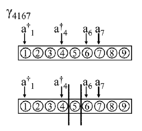
The way forward is to observe that we are not tied to using a single canonical form/block configuration for the DMRG wavefunction, but rather, can evaluate a density matrix element $\gamma_{ijkl}$ at any canonical form/block configuration that is convenient. As we have described above, a given DMRG wavefunction can be expressed in the canonical form/block-configuration associated with any site. By taking advantage of this flexibility, we can reduce the memory requirements once again back to $O(M^{2}k^{2})$, i.e. the same as in the standard quantum chemical DMRG algorithm. Given a two-particle density matrix element $\langle a^{\dagger}_{i}a^{\dagger}_{j}a_{k}a_{l}\rangle$, where, say $i\leq j\leq k\leq l$, we choose a block configuration such that $i,j$ lie in the left block and sites $k,l$ lie in the right block, i.e. $\framebox{$\ldots\bullet_{i}\ldots\bullet_{j}\ldots$}\ \bullet_{p}\ \framebox{$\ldots\bullet_{k}\ldots\bullet_{l}\ldots$}$. The corresponding matrix element may then be evaluated using $a^{\dagger}_{i}a^{\dagger}_{j}$ on the left block, and $a_{k}a_{l}$ on the right block, and thus no operator matrices with more than two orbital indices appear on either block (see Figure 1). By the appropriate choice of partitioning between the left and right blocks, we can arrange things such that we never manipulate operators with more than two orbital labels on either the left or right blocks for any $ijkl$. During a DMRG sweep we iterate through all block configurations where the dividing site $\bullet_{p}$ ranges from site 2 to site $k-1$. At each block configuration, we then evaluate all the two-particle density matrix elements which do not require more than two-index operators on either the left or right blocks, and assemble the contributions of all the block configurations at the end of the DMRG sweep.

Along these lines, we can formulate an efficient algorithm to evaluate the two-particle density matrix with a total per-sweep computational cost of $O(M^{3}k^{4})$ and a memory cost of $O(M^{2}k^{2})$. The pseudocode is given in Algs. (1), (2). Alg. (1) describes how to partition the evaluation of different density matrix elements amongst the block configurations as we traverse a DMRG sweep. The actual calculation of the density matrix elements is carried out by the function Compute in Alg. (2), which computes all density matrix elements that may be assembled from $nl$ index operators on the left block, $np$ index operators on site $p$, and $nr$ index operators on the right block.

Algorithm 1 Two-particle density matrix evaluation showing how the two-particle density matrix is assembled across a DMRG sweep.

  special treatment for first configuration $\framebox{$\bullet_{1}$}\ \bullet_{2}\ \framebox{$\bullet_{3}\ldots\bullet_{k}$}$

  $left$$=$ site $1$, $sitep$$=$ site $2$, $right$$=$ sites $3\ldots k$

  Compute(4, 0, 0, $left$, $sitep$, $right$)

  Compute(3, 1, 0, $left$, $sitep$, $right$)

  Compute(3, 0, 1, $left$, $sitep$, $right$)

  Compute(2, 1, 1, $left$, $sitep$, $right$)

  sweep through block configurations $\framebox{$\bullet_{1}\ldots\bullet_{p-1}$}\ \bullet_{p}\ \framebox{$\bullet_{p+1}\ldots\bullet_{k}$}$

  for $sitep$$=$ 2 to k-1 do

     $left$$=$ sites $1\ldots p-1$, $right$$=$ sites $p+1\ldots k$

     Compute(1, 2, 1, $left$, $sitep$, $right$)

     Compute(2, 1, 1, $left$, $sitep$, $right$)

     Compute(2, 2, 0, $left$, $sitep$, $right$)

     Compute(1, 3, 0, $left$, $sitep$, $right$)

     Compute(0, 3, 1, $left$, $sitep$, $right$)

     Compute(0, 4, 0, $left$, $sitep$, $right$)

  end for

  special treatment for final configuration $\framebox{$\bullet_{1}\ldots\bullet_{k-2}$}\ \bullet_{k-1}\ \framebox{$\bullet_{k}$}$

  $left$$=$ sites $1\ldots k-2$, $sitep$$=$ site $k-1$, $right$$=$ site $k$

  Compute(0, 0, 4, $left$, $sitep$, $right$)

  Compute(0, 1, 3, $left$, $sitep$, $right$)

  Compute(1, 0, 3, $left$, $sitep$, $right$)

  Compute(0, 2, 2, $left$, $sitep$, $right$)

  Compute(2, 0, 2, $left$, $sitep$, $right$)

  Compute(1, 1, 2, $left$, $sitep$, $right$)

  Compute(1, 2, 1, $left$, $sitep$, $right$)

Algorithm 2 $\mbox{\sc Compute}(nl,np,nr,left,sitep,right)$. Note $nl,np,nr\leq 2$ and $nl+np+nr=4$, i.e. the number of indices in the two-particle density matrix $\gamma$.

  for all $opl$$=$ operators with $nl$ indices on block $left$ do

     (If parallel, loop only over $opl$ stored on current proc)

     for all $opp$$=$ operators with $np$ indices on block $sitep$ do

        for all $opr$$=$ operators with $nr$ indices on block $right$ do

           $\gamma(np,nl,nr)$ $=$ $\text{parity}(opl,opp,opr)\times\langle\Psi|opl\otimes opp\otimes opr|\Psi\rangle$

        end for

     end for

  end for

  (If parallel, accumulate contributions from all procs to root processor)

An attractive feature of the quantum chemical DMRG algorithm is the high level of parallelisability, which we have described in detail in Ref. Chan2004 . In our implementation, the loops over operators in Alg. (2) are trivially parallelised because of how our operators are divided across processors in our original formulation Chan2004 . For example, the dominant computational cost of the two-particle density matrix evaluation comes from $\mbox{\sc Compute}(2,1,1,left,sitep,right)$ in Alg. (1), which costs $O(M^{3}k^{4})$ per DMRG sweep. However, in our parallel DMRG implementation, the two index operators $opl$ on the left block, namely $a^{\dagger}_{i}a_{j}$ and $a_{i}a_{j}$, are divided across the processors, while the corresponding one index operators $opp,opr$ are replicated on all processors, and thus we can easily parallelise over the first $opl$ loop in Alg. (2). This leads to a final computational cost per sweep of $O(M^{3}k^{4}/n_{p})$ with a communication cost of $O(k^{4}\ln n_{p})$, where $n_{p}$ is the number of processors.

II.3 Orbital step and integral transformation

As described earlier, the DMRG wavefunction is primarily efficient at capturing static correlation and consequently we employ an active space DMRG description of the electronic structure, the purpose of the orbital optimisation then being to obtain the best form of the active space. Recall that the active space is defined by partitioning the orbitals into three sets, closed-shell orbitals which remain doubly occupied in all DMRG configurations, active orbitals which form the product active space $\{n_{1}\}\otimes\ldots\otimes\{n_{k}\}$ in the DMRG wavefunction expansion (10), and external orbitals, which remain unoccupied in all DMRG configurations. With this partitioning, the active space DMRG wavefunction is determined with respect to the active space Hamiltonian

$$H^{\mathrm{act}}=E^{\mathrm{closed}}+\sum_{ij}t^{\mathrm{act}}_{ij}a^{\dagger}_{i}a_{j}+\sum_{ijkl}v_{ijkl}a^{\dagger}_{i}a^{\dagger}_{j}a_{k}a_{l}$$ (25)

where indices $i,j$ are limited to the active orbitals and the modified one-particle integrals $t^{\text{act}}_{ij}$ and closed-shell energy are given respectively by

$$E^{\mathrm{closed}} =\sum_{c}t_{cc}+\sum_{cc^{\prime}}(v_{cc^{\prime}c^{\prime}c}-v_{cc^{\prime}cc^{\prime}})$$ (26)

$$t^{\mathrm{act}}_{ij} =t_{ij}+2\sum_{c}(v_{iccj}-v_{icjc})$$ (27)

where $c,c^{\prime}$ denote the closed-shell indices.

Orbital optimisation chooses the best form of the active orbitals by minimising the energy of the DMRG wavefunction with respect to the active and closed-shell orbitals. This is the basic idea behind the Complete-Active-Space Self-Consistent Field (CASSCF) description of electronic structure. In CASSCF, the active space wavefunction is the exact eigenfunction of the active space Hamiltonian (25) and is thus invariant with respect to active-active orbital rotations. In the corresponding orbital optimised DMRG-CASSCF, the accuracy of our active space DMRG wavefunction depends on the size of $M$, but in this study we will use sufficiently large $M$ so that our wavefunction is nearly an exact eigenfunction of the active space Hamiltonian, and we will similarly omit active-active rotations.

The algorithm we use for orbital optimisation is an Augmented Hessian Newton Raphson scheme similar to that used in modern CASSCF implementations knowles ; yeager1982nra ; lengsfieldiii1981som . The orbital rotations are parameterised by the anti-hermitian amplitudes $A$ in Eq. (5), and the derivative with respect to these amplitudes is evaluated from the one- and two-particle density matrices from the DMRG calculation. However, as the DMRG enables the use of larger active spaces than in traditional CASSCF studies and consequently we can expect to have a larger number of correlating external and closed-shell orbitals, we have focused on an efficient parallel implementation of the orbital optimisation. Here the primary task is to parallelise the four-index transformation which is performed after each orbital rotation to generate the two-electron integrals in the basis of the rotated orbitals. We now describe how this is done.

Say we have a coefficient matrix $\bm{U}$ giving the expansion coefficients for our rotated orbitals in terms of the starting atomic orbitals. Then, the transformed integrals $v_{pqrs}$ are obtained from the atomic orbital integrals $v^{\text{AO}}_{\mu\nu\kappa\lambda}$ through (assuming real coefficients, for simplicity)

$$v_{pqrs}=\sum_{\mu\nu\kappa\lambda}U_{p\mu}U_{q\nu}U_{r\kappa}U_{s\lambda}v^{\mathrm{AO}}_{\mu\nu\kappa\lambda}$$ (28)

As is well known, the four-index transformation should be carried out in four quarter-transformation steps corresponding to the four contractions with the coefficient matrices above. In our parallel transformation scheme, we consider the four steps in two stages; in the first stage we perform two quarter-transformations to construct half-transformed Coulomb and exchange intermediates $J,K$

$$J_{ab}(\nu,\kappa)=\sum_{\mu\lambda}U_{a\mu}U_{b\lambda}v^{\mathrm{AO}}_{\mu\nu\kappa\lambda}$$ (29)

$$K_{ab}(\nu,\kappa)=\sum_{\mu\lambda}U_{a\mu}U_{b\lambda}v^{\mathrm{AO}}_{\mu\nu\lambda\kappa}$$ (30)

while in the second stage, we perform the remaining quarter transformations on the $J$, $K$ intermediates to obtain the final integrals

$$[J_{ab}]_{pq} =v_{apqb}=\sum_{\nu\kappa}J_{ab}(\nu,\kappa)U_{p\nu}U_{q\kappa}$$ (31)

$$[K_{ab}]_{pq} =v_{apbq}=\sum_{\nu\kappa}K_{ab}(\nu,\kappa)U_{p\nu}U_{q\kappa}$$ (32)

Note that for the purposes of optimising the active orbitals, we only need the integrals that appear in the augmented Hessian. Thus, the $ab$ indices in (29), (30) only need to run over the active orbitals while the $pq$ indices need to run over all the closed-shell, active, and external orbitals.

In the first stage, we parallelise the construction of the $J,K$ intermediates by dividing up the intermediates according to their untransformed AO indices. For example, the construction of $J_{ab}(\nu,\kappa)$ is divided amongst the processors according to the pair of indices $(\nu,\kappa)$; each processor is then responsible for constructing the $J$ intermediates for all $(\bar{\nu},\bar{\kappa})\in\text{proc}$. This allows us to also partition the AO integrals amongst the processors according to the same divided pair of indices ($\bar{\nu},\bar{\kappa}$); e.g. to construct $J_{ab}(\bar{\nu},\bar{\kappa})$ for $(\bar{\nu},\bar{\kappa})\in\text{proc}$ we only need AO integrals such as $v^{\text{AO}}_{\mu\bar{\nu}\bar{\kappa}\lambda}$ for $(\bar{\nu},\bar{\kappa})\in\text{proc}$ to be stored on that processor.

Once all $J$ and $K$ intermediates are constructed, we parallelise the second stage with respect to the transformed $ab$ indices of the $J$, $K$ intermediates. Thus $ab$ is divided amongst the processors, and each processor constructs the final integrals $v_{\bar{a}pq\bar{b}},v_{\bar{a}p\bar{b}q}$ for all $\{\bar{a}\bar{b}\}\in\text{proc}$. Since the first stage is parallelised over a pair of AO indices ($\nu,\kappa$) (and the $J$ and $K$ intermediates are divided across the processors accordingly) while the second stage is parallelised over the two transformed indices ($ab$), we need to redistribute the intermediates $J$ and $K$ amongst the processors between the first and second stages. This is the main communication step.

In addition to above parallelisation, further efficiencies can be gained by using the permutational and spatial symmetries of the integrals. Our complete parallelised algorithm, which uses these symmetries, is presented in pseudocode in Alg. (3). The cost of the four-index integral transformation as implemented is $O((K^{4}k+K^{3}k^{2})/n_{p})$ for CPU, $O((K^{4}+K^{2}k^{2})/n_{p})$ for disk space, $O(K^{2}k^{2}/n_{p})$ for memory, and $O(K^{2}k^{2})$ for overall communication, where $K$ is the total number of orbitals, $k$ is the number of active orbitals, and $n_{p}$ is the number of processors.

To complete our efficient implementation of orbital optimisation, we have also parallelised the remaining steps in the Augmented Hessian Newton-Raphson solver. These additional steps take up only a small part of the computational time and have an overall cost $O(K^{2}k^{3}/n_{p})$ for CPU time, $O(K^{2}k^{2}/n_{p})$ for memory, $O(Kk)$ for communication.

Algorithm 3 Parallel four-index integral transformation algorithm.

  Stage 1: Assemble $J$ and $K$ intermediates

  Divide AO integrals $v^{\text{AO}}_{\mu\nu\kappa\lambda}$ by a factor $(2-\delta_{\mu\lambda})(2-\delta_{\nu\kappa})(2-\delta_{\mu\lambda,\nu\kappa})$

  for $\bar{\nu},\bar{\kappa}\,(\bar{\nu}\geq\bar{\kappa})\in\text{proc}$ do

     for $a,\mu,\lambda$   s.t. $\mu\geq\lambda$, $\mu\lambda\geq\bar{\nu}\bar{\kappa}$  do

        $M^{a}_{\mu}(\bar{\nu},\bar{\kappa})$ += $v^{\mathrm{AO}}_{\mu\bar{\nu}\bar{\kappa}\lambda}\,U_{a\lambda}$;     $N^{a}_{\lambda}(\bar{\nu},\bar{\kappa})$ += $v^{\mathrm{AO}}_{\mu\bar{\nu}\bar{\kappa}\lambda}\,U_{a\mu}$

        $N^{a}_{\mu}(\bar{\nu},\bar{\kappa})$ += $v^{\mathrm{AO}}_{\mu\bar{\kappa}\bar{\nu}\lambda}\,U_{a\lambda}$;     $N^{a}_{\lambda}(\bar{\nu},\bar{\kappa})$ += $v^{\mathrm{AO}}_{\mu\bar{\kappa}\bar{\nu}\lambda}\,U_{a\mu}$

     end for

     for $a,\lambda$ do

        $N^{a}_{\lambda}(\bar{\nu},\bar{\kappa})$ += $M^{a}_{\lambda}(\bar{\nu},\bar{\kappa})$

     end for

     for $a,\mu,\lambda$   s.t. $\mu\geq\lambda$, $\bar{\nu}\bar{\kappa}\geq\mu\lambda$  do

        $L^{a}_{\mu}(\bar{\nu},\bar{\kappa})$ += $v^{\mathrm{AO}}_{\bar{\nu}\mu\lambda\bar{\kappa}}\,U_{a\lambda}$

     end for

     for $a,b,\lambda$   s.t. $a\geq b$ do

        $J_{ab}(\bar{\nu},\bar{\kappa})$ += $M^{a}_{\lambda}(\bar{\nu},\bar{\kappa})\,U_{b\lambda}+M^{b}_{\lambda}(\bar{\nu},\bar{\kappa})\,U_{a\lambda}+L^{a}_{\lambda}(\bar{\nu},\bar{\kappa})\,U_{b\lambda}+L^{b}_{\lambda}(\bar{\nu},\bar{\kappa})\,U_{a\lambda}$

     end for

     for $a,b,\lambda$ do

        $K_{ab}(\bar{\nu},\lambda)$ += $N^{a}_{\lambda}(\bar{\nu},\bar{\kappa})\,U_{b\bar{\kappa}}$

     end for

  end for

  for $a,b$   s.t. $a\geq b$ do

     write $J_{ab}$, $K_{ab}$, and $K_{ba}$ on disk

  end for

  Stage 2: Redistribute $J$ and $K$, transform to final integrals

  for $a,b\,(a\geq b)$ do

     read $J_{ab}$, $K_{ab}$, $K_{ba}$ from disk and send to proc$(a,b)$

  end for

  for $\bar{a},\bar{b}\,(\bar{a}\geq\bar{b})\in$ proc, $\nu,\kappa\,(\nu\geq\kappa)$ do

     $J_{\bar{a}\bar{b}}(\kappa,\nu)+=J_{\bar{a}\bar{b}}(\nu,\kappa)$

  end for

  for $\bar{a},\bar{b}\,(\bar{a}\geq\bar{b})\in$ proc, $\nu,\kappa$ do

     $K_{\bar{a}\bar{b}}(\kappa,\nu)+=K_{\bar{b}\bar{a}}(\nu,\kappa)$

  end for

  for $\bar{a},\bar{b}\,(\bar{a}\geq\bar{b})\in$ proc, $p,q,\nu,\kappa$ do

     $v_{\bar{a}pq\bar{b}}$ += $J_{\bar{a}\bar{b}}(\nu,\kappa)\,U_{p\nu}U_{q\kappa}$ (eqn. (31))

     $v_{\bar{a}p\bar{b}q}$ += $K_{\bar{a}\bar{b}}(\nu,\kappa)\,U_{p\nu}U_{q\kappa}$ (eqn. (32))

  end for

II.4 Complete Orbital Optimised DMRG-CASSCF Algorithm

With the description of the density matrix evaluation in Sec. II.2 and the orbital optimisation and integral transformation in Sec. II.3, we now have the basic ingredients to perform the DMRG-CASSCF algorithm, according to the general outline in Sec. II.1.

There is one final ingredient however, the secret ingredient. As the DMRG works best in a localised basis (particularly in larger systems) it is beneficial to localise the active space after each orbital optimisation. We have done this using the Pipek-Mezey procedure pipekmezey ; the active-space integrals are first transformed into this local basis before being input into the DMRG calculation. In total therefore, the complete DMRG-CASSCF algorithm is as follows:

1. Localise the active space orbitals.

2. Transform the AO integrals to the active space basis and build the active space Hamiltonian.

3. Perform the DMRG calculation using the active space Hamiltonian.

4. From the converged DMRG wavefunctions at each block configuration, assemble the one- and two-particle density matrices.

5. Using the density matrices, obtain the orbital gradient and orbital step from the Augmented Hessian Newton-Raphson solver.

6. From the orbital step, determine the new active space orbitals.

7. Goto 1. until convergence in the energy.

Steps 1.-6. constitute a single DMRG-CASSCF macro-iteration.

III Applications

III.1 Long Polyenes

III.1.1 Background

Polyenes are the simplest conjugated systems, consisting of alternating singly and doubly bonded carbons arranged in a chain. They are valuable models not only to understand conjugated polymers of materials interest (e.g. poly-acetylene is simply an infinite polyene) but also biological molecules such as the carotenoid and retinal families of pigments involved in photosynthesis and vision. In these systems, the functionality of the molecules relies on the low-lying $\pi$-$\pi^{*}$ excited states of the conjugated backbone, which serve as the conduits for energy transfer. The excited states are labelled by their symmetry under the $C_{2h}$ point group, giving rise to $A_{g},B_{g},A_{u},B_{u}$ symmetry labels. Furthermore, they are usually given an additional $+/-$ label to indicate their approximate particle-hole symmetry. In Hamiltonians (such as the Hückel Hamiltonian) which support symmetric sets of energy states around the Fermi level, there is an additional symmetry associated with rotating the molecular orbital diagram so that the bonding and anti-bonding levels swap places pariser . Although particle-hole symmetry is not a true symmetry of the ab-initio electronic Hamiltonian, it is still customary to use such labels for the polyenes, in particular, because the $+/-$ states have very different qualitative electronic structure; valence bond studies of the Hubbard model hubbardmodel show that the $+$ states consist mainly of ionic valence bond structures, while the $-$ states consist mainly of covalent valence bond structures kurashige ; Ramasesha1996 ; tavan .

In this study we have looked only at singlet states and henceforth we shall be considering singlet states only. The ground state of the polyenes is known to always be of $A_{g}^{-}$ symmetry. The lowest dipole-allowed singlet transition, which has a predominantly HOMO$\to$LUMO excitation character, has $B_{u}^{+}$ symmetry. However, contrary to what one might expect, this $1A_{g}^{-}\rightarrow 1B_{u}^{+}$ transition is not the lowest singlet transition kohler ; kohler1 . Rather, as shown by Kohler et al. in octa-tetraene kohler , there is a lower dipole forbidden excitation, later identified as the $2A_{g}^{-}$ state, which can be rationalised in valence bond language as arising from a pair of singlet-triplet excitations in the two separate double bonds that recouple to form a singlet state andres ; dunningshavitt ; cave ; cavedavidson ; brooks ; petrongolo ; lappe ; lasaga ; bachler . Following the observation of the $2A_{g}^{-}$ state in octa-tetraene, there has been much debate over the correct ordering of the $2A_{g}^{-}$ and $1B_{u}^{+}$ excited states in the shorter polyenes, compounded both by experimental difficulties in observing the dipole-forbidden $2A_{g}^{-}$ state as well as theoretical challenges in achieving a balanced description of the two states, which are dominated by very different kinds of correlation, namely static correlation in the $2A_{g}^{-}$ state and dynamic correlation in the $1B_{u}^{+}$ state. In longer polyenes and the biologically active carotenoid and retinal pigments, questions about the low-lying spectrum are not restricted simply to the $2A_{g}^{-}$ and $1B_{u}^{+}$ state ordering. Recent studies using Resonance Raman excitation profiles (RREP) and electronic absorption spectroscopy on substituted polyenes in the carotenoid family, have indicated the presence of additional dark states below the $1B_{u}^{+}$ state sashima ; sashima2 ; fujii ; onaka ; furuichi . In particular, for the all-trans-carotenoids with (the number of double bonds) $n=9-11$, Sashima et al. observed a $1B_{u}^{-}$ state between the $2A_{g}$ and $1B_{u}^{+}$ sashima ; cogdellscience . More recently, Furuichi et al. observed a $3A_{g}^{-}$ level between the $1B_{u}^{-}$ and $1B_{u}^{+}$ states in carotenoids with $n=11-13$, and assigned the tentative state ordering of $1A_{g}^{-}<2A_{g}^{-}<1B_{u}^{-}<3A_{g}^{-}<1B_{u}^{+}$ furuichi . The assignment was made by extrapolating from the earlier PPP-MRDCI calculations by Tavan and Schulten on short polyenes ($n=2-8$), which had predicted the existence of these additional states tavan .

To better understand the electronic structure of these low-lying states, we would ideally like to be able to carry out an ab-initio multireference calculation, using the complete $\pi$-valence space. However, the large number of active $\pi$ orbitals in the longer polyenes means that it is not possible to perform such calculations with traditional CAS algorithms for these systems. Hirao and coworkers hirao ; kurashige carried out incomplete valence CASSCF and CASCI-MRMP using a (10,10) active space on the polyene series up to $\text{C}_{28}\text{H}_{30}$ and observed reasonable agreement with experiment. However, with our new orbital optimised DMRG-CASSCF procedure, we can now re-examine the low-lying excitations in these systems correlating the complete $\pi$- valence space even for the longer polyenes and carotenoids.

III.1.2 Computational details

The polyene molecular geometries for $\text{C}_{8}\text{H}_{10},\text{C}_{12}\text{H}_{14},\text{C}_{16}\text{H}_{18},\text{C}_{20}\text{H}_{22},\text{C}_{24}\text{H}_{26}$ were optimised at the density functional level using the B3LYP functional becke1993dft ; lee1988dcs as implemented in Gaussian03 gaussian . The polyene molecules were constrained to have $C_{2h}$ symmetry, with the $C_{2}$ axis as the $z$-axis. The cc-pVDZ basis cc-pvdz was used for all calculations.

In our DMRG-CASSCF calculations we used a complete $\pi$-valence space i.e. in $\text{C}_{24}\text{H}_{26}$, this was a (24, 24) active space. To generate this active space, we first performed a restricted Hartree-Fock calculation in PSI3 PSI3 ; crawford2007sp to obtain canonical Hartree-Fock molecular orbitals. From these molecular orbitals, we could not trivially identify appropriate $\pi$ anti-bonding active orbitals because of significant $2p$-$3p$ mixing. We constructed the anti-bonding component of the active space as a set of projected atomic orbitals, by first projecting out the $\pi$ bonding space from a set of $2p_{z}$ atomic orbitals. These projected atomic orbitals were then symmetrically orthogonalised, then relocalised together with the bonding molecular orbitals (using the Pipek-Mezey procedure pipekmezey ) to yield the complete active space in our calculations. The final set of active orbitals generated in this way resemble an orthogonal set of $2p_{z}$ orbitals.

Note that our initial active space does not correspond precisely to an active space obtained by selecting Hartree-Fock canonical orbitals. Thus DMRG energies obtained before orbital optimisation do not correspond to typical CASCI energies, but instead to CASCI energies obtained in our projected-atomic orbital (PAO) virtual space. This distinction is noted in our tables with the abbreviation DMRG-PAO-CASCI. After orbital optimisation, however, our DMRG-CASSCF energies do correspond to true CASSCF energies, up to the accuracy of the DMRG calculation.

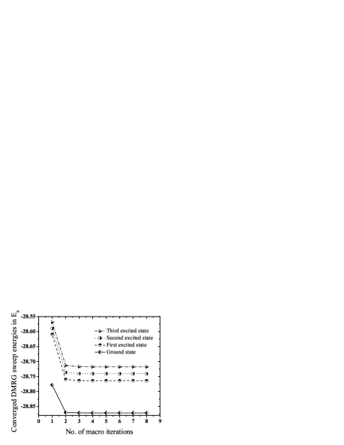
We carried out state-averaged DMRG-CASSCF calculations in the above active space with the one-site DMRG algorithm with $M=250$ and averaging over the $4$ lowest eigenstates. The DMRG sweeps were converged to $10^{-10}E_{h}$ in the DMRG energy, which took roughly 30 DMRG sweeps. The number of renormalised states was increased smoothly from a starting value of $M=50$ to the final value of $M=250$. To aid the convergence of the DMRG sweeps in the one-site algorithm, we applied a system-environment perturbation as described in Ref. white-onedot , with a starting magnitude of $10^{-3}$ that smoothly decreased to 0 after 20 sweeps. We estimate the remaining error in the DMRG energies at the $M=250$ level from the exact Full-Configuration Interaction energies in the same active space to be less than $0.1$m$E_{h}$. Our DMRG calculations were combined with orbital rotation in a macro-iteration consisting of a converged DMRG calculation, an Augmented-Hessian step based orbital rotation, integral transformation, and orbital localisation, as described in Sec. II.4. Typically 10-15 macro-iterations of the complete DMRG/orbital optimisation cycle were necessary to converge the energies to a tolerance of better than $10^{-6}E_{h}$. The convergence of the state energies with the number of macro-iterations is shown in Fig. 3.

The spatial and spin symmetries of excited states were assigned as follows. Firstly, all excited states were restricted to be of singlet spin symmetry through the application of a shift $\lambda(\hat{S}^{2}-\langle S\rangle(\langle S\rangle+1)$ with $\lambda=0.5$ Moritz2005rel . To obtain the spatial symmetry, the ground state was assumed to be $1A_{g}^{-}$ as established by prior experimental and theoretical work. To determine whether the excited states were of $A_{g}$ or $B_{u}$ symmetry the transition dipole matrices were calculated between the states. Additionally, to determine the approximate particle-hole $+$ or $-$ symmetry we examined the magnitude of the transition dipoles; large transition dipoles for an allowed transition indicated that the transition involved a change of particle-hole symmetry between the states.

III.1.3 Discussion

Figure 2: DMRG-CASSCF excitation energies in $eV$ for the $2A_{g}^{-}$, $1B_{u}^{-}$ and $3A_{g}^{-}$ states in the conjugated polyenes $\text{C}_{8}\text{H}_{10}$ to $\text{C}_{24}\text{H}_{26}$ .

Figure 3: Converged DMRG sweep energies in Hartrees vs number of orbital optimisation macro iterations in $\text{C}_{20}\text{H}_{22}$.

Figure 4: Change in CASSCF energies of the low-lying states of $\text{C}_{12}\text{H}_{14}$ as a function of increasing the active space from (4,4) to (12,12) (i.e. complete valence active space).

Table 1: Energies, symmetries, and oscillator strengths for the lowest lying singlet excited states in conjugated polyenes. The DMRG-PAO-CASCI and DMRG-CASSCF entries for the $1A_{g}^{-}$ ground-states give the total energy in $E_{h}$; the other entries give the excitation energies from the ground state in $eV$. The estimated error of the DMRG-CASSCF energies from the exact CASSCF energies in the same active space is less than 0.1m$E_{h}$. The notation $(n,m)$ denotes the active space used in the DMRG-PAO-CASCI and DMRG-CASSCF calculations. Oscillator strengths are in $a.u.$ for the ground-state, excited state transition. The CASCI-MRMP excitation energies are from Kurashige et al. kurashige ; note that these used at most a (10,10) active space. The experimental numbers in brackets are from measurements on the substituted polyene, spheroidene furuichi .

Polyenes	Symmetry	DMRG	DMRG	Oscillator	CASCI-MRMP	Expt
		PAO-CASCI	CASSCF	Strength
$\text{C}_{8}\text{H}_{10}$	$1A_{g}^{-}$	$-308.823021$	$-308.825879$
$(8,8)$	$2A_{g}^{-}$	$6.33$	$4.69$	Forbidden	$4.26$	$3.54$
	$1B_{u}^{-}$	$7.49$	$5.88$	$0.0565$	$5.30$
	$3A_{g}^{-}$	$7.95$	$6.60$	Forbidden	$7.20$
$\text{C}_{12}\text{H}_{14}$	$1A_{g}^{-}$	$-462.661260$	$-462.670591$
$(12,12)$	$2A_{g}^{-}$	$5.40$	$3.76$	Forbidden	$3.19$
	$1B_{u}^{-}$	$6.30$	$4.74$	$0.0620$	$3.98$
	$3A_{g}^{-}$	$7.01$	$5.59$	Forbidden	$5.12$
$\text{C}_{16}\text{H}_{18}$	$1A_{g}^{-}$	$-616.499262$	$-616.514639$
$(16,16)$	$2A_{g}^{-}$	$4.90$	$3.25$	Forbidden	$2.50$	$2.21$
	$1B_{u}^{-}$	$5.60$	$4.03$	$0.0502$	$3.10$
	$3A_{g}^{-}$	$6.28$	$4.78$	Forbidden	$3.99$
$\text{C}_{20}\text{H}_{22}$	$1A_{g}^{-}$	$-770.337112$	$-770.358327$
$(20,20)$	$2A_{g}^{-}$	$4.60$	$2.93$	Forbidden	$2.04$	$(1.76)$
	$1B_{u}^{-}$	$5.15$	$3.57$	$0.0427$	$2.51$	$(2.18)$
	$3A_{g}^{-}$	$5.71$	$4.20$	Forbidden	$3.11$	$(2.47)$
$\text{C}_{24}\text{H}_{26}$	$1A_{g}^{-}$	$-924.174795$	$-924.201821$
$(24,24)$	$2A_{g}^{-}$	$4.42$	$2.73$	Forbidden	$1.70$	$(1.53)$
	$1B_{u}^{-}$	$4.85$	$3.25$	$0.0384$	$2.05$	$(1.80)$
	$3A_{g}^{-}$	$5.31$	$3.78$	Forbidden	$2.45$	$(2.02)$

In Table 1 we present the energies, symmetries, and oscillator strengths for the ground state and first 3 excitations in the polyenes from $\text{C}_{8}\text{H}_{10}$ to $\text{C}_{24}\text{H}_{26}$. For comparison, we also give the excitation energies obtained from the CASCI-MRMP calculations of Kurashige et al. kurashige , as well as the experimental energies where available. (Note that in $\text{C}_{20}\text{H}_{22}$, the experimental excitation energies were obtained from the carotenoid spheroidene, which has a $\text{C}_{20}$ conjugated backbone).

We see that while our complete $\pi$-valence active space DMRG-CASSCF calculations generally overestimate the excitation energies, they reproduce the correct experimental ordering of the lowest excited states with the exception of the missing $1B_{u}^{+}$ state (the HOMO-LUMO excitation), which should lie below the $3A_{g}^{-}$ in the shorter polyenes such as $\text{C}_{8}\text{H}_{10}$. If we perform a state-averaged DMRG-CASSCF with 5 states in $\text{C}_{8}\text{H}_{10}$, we find that the $1B_{u}^{+}$ state lies immediately above the $3A_{g}^{-}$. This may seem strange given that CASSCF is generally believed to yield qualitatively correct electronic structure, but it reflects the wisdom from earlier studies on butadiene that $\sigma$-$\pi$ correlation is very strong in the $1B_{u}^{+}$ state and must be included to obtain the correct balance between Rydberg and valence character cavedavidson ; Roos1993 ; Roos1989 ; dunningshavitt . Comparing with the calculations of Kurashige et al. kurashige , which despite having an incomplete valence active space include dynamic $\sigma$-$\pi$ correlation through MRMP perturbation theory hirao_mrmp , further indicates that $\sigma$-$\pi$ correlation would also lower the excitation energies of our other excited states.

To better understand the effect of using a complete $\pi$ valence space on the excitation energies, we have performed some small benchmark CASSCF calculations on $\text{C}_{12}\text{H}_{14}$ with $4-12$ active orbitals. These results are presented in Fig. 4. As can be seen, there is a very strong dependence of the excitation energies on the size of the active space, and even the order of the excitations changes. Thus, while an incomplete valence active space can yield an excited state ordering in better agreement with experiment, one is tempted to argue that it does not do so for the right reason.

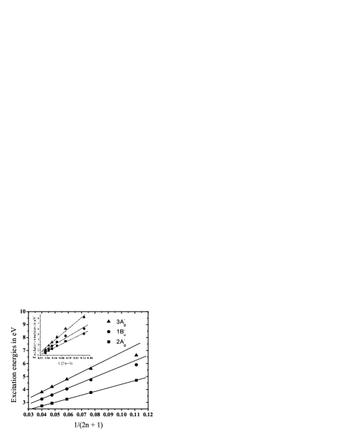
In Fig. 5, we plot our DMRG-CASSCF excitation energies as a function of the inverse chain length of the polyenes. Also shown (as an inset) is the same plot for the excitation energies obtained by Kurashige et al. kurashige . It is easy to show that in a finite Hückel model with $n$ sites, the excitation energies have a $\sin(k\pi/2(2n+1))$ chain length dependence, where $k$ is a quasi-momentum number that labels the excitation. For long chains, this implies an asymptotic linear dependence on the inverse chain length $1/(2n+1)$. Tavan and Schulten conjectured that this asymptotic behaviour held also in interacting systems, and presented evidence from MRD-CI calculations on short-chain Hubbard ($n$ up to 7) and Pariser-Parr-Pople models ($n$ up to 8) to support the conjecture tavan2 . The experimental Resonance Raman excitation profiles from Sashima et al. sashima and Furuichi et al. furuichi were also approximately fitted to the same inverse chain length behaviour, although only over a small range of $n=9-13$. We see from our results that while the $2A_{g}^{-}$ and $1B_{u}^{-}$ excitation energies fit the asymptotic $1/(2n+1)$ behaviour well, the $3A_{g}^{-}$ state shows curvature more indicative of the sinusoidal dependence expected when $k\sim 2n+1$. This is consistent with interpreting the $3A_{g}^{-}$ as an excitation labelled by a larger quasi-momentum than $2A_{g}^{-}$. Interestingly, the excitation energies of Kurashige et al. show quite different chain-length dependence, with all three states showing much stronger curvature when their excitation energies are plotted against $1/(2n+1)$ in Fig. 5 (inlay). Fitting our excitation energies for $\text{C}_{16}\text{H}_{20}$, $\text{C}_{20}\text{H}_{24}$, $\text{C}_{24}\text{H}_{26}$ ($n=8-12$) to the asymptotic dependence $1/(2n+1)$, we obtain slopes of 27.67eV, 41.34eV, 52.63eV for the $2A_{g}^{-}$, $1B_{u}^{-}$, $3A_{g}^{-}$ excitations, in reasonable agreement with the experimental slopes of 31.39eV, 49.07eV and 59.63eV.

Figure 5: DMRG-CASSCF excitation energies for the low-lying singlet excited states of polyenes ranging from $\text{C}_{12}\text{H}_{14}$ to $\text{C}_{24}\text{H}_{26}$. The excitation energies are plotted against $1/(2n+1)$ where $n$ is the number of double bonds. The ratio of the slopes for the different states is found to be $2:3.0:3.8$ as compared to $2:3.1:3.8$ experimentally. Inset: same plot for the CASCI-MRMP excitation energies from Kurashige et al. kurashige . As can be seen, these show a different and less linear-dependence on $1/(2n+1)$.

Table 2: Single particle nature of the polyene excitations (in %). For a given excited state (e.g. $2A_{g}^{-}$), the excitation weight of the transition $i\to j$ is given by $[\langle 1A_{g}^{-}|a^{\dagger}_{i}a_{j}|2A_{g}^{-}\rangle]^{2}$. The total excitation weight is the sum of weights for all transitions; $100\%$ indicates that the given excited state corresponds entirely to single excitations from the ground state. The transition labels $n\rightarrow m^{\prime}$ are interpreted as follows: 1, 2, 3 $\ldots$ denote HOMO, HOMO-1, HOMO-2 $\ldots$ natural orbitals, while $1^{\prime}$, $2^{\prime}$, $3^{\prime}$ denote LUMO, LUMO+1,LUMO+2 natural orbitals. As the polyenes increase in length, the total weight of the single excitations in the low-lying states becomes very small, $<16\%$.

State	Excitation	No. of conjugated double bonds
	weight	$4$	$6$	$8$	$10$	$12$
$2A_{g}^{-}$	$2\rightarrow 1^{\prime}$	$10.9$	$8.6$	$6.6$	$5.3$	$4.3$
	$1\rightarrow 2^{\prime}$	$6.7$	$5.9$	$4.8$	$4.0$	$3.3$
	Total	$20.0$	$18.0$	$15.4$	$13.5$	$12.1$
$1B_{u}^{-}$	$3\rightarrow 1^{\prime}$	$14.5$	$10.2$	$7.9$	$6.3$	$5.2$
	$1\rightarrow 3^{\prime}$	$7.0$	$5.6$	$4.6$	$3.9$	$3.3$
	Total	$25.3$	$21.8$	$18.6$	$16.3$	$14.7$
$3A_{g}^{-}$	$4\rightarrow 1^{\prime}$	$21.3$	$12.8$	$9.3$	$7.1$	$5.6$
	$1\rightarrow 4^{\prime}$	$8.2$	$6.0$	$4.7$	$3.8$	$3.1$
	Total	$32.9$	$25.0$	$20.9$	$18.0$	$15.9$

From the one particle transition density matrices we can analyse the single-particle character of our excitations. Given the density matrix element $w_{ij}=\langle\text{g.s.}|a^{\dagger}_{i}a_{j}|\text{excited}\rangle$ where $i,j$ are natural orbitals in the ground state, we define the weight of the $i\to j$ excitation as $w_{ij}^{2}$. The total single excitation weight is then $\sum_{ij}w_{ij}^{2}$. In Table 2 we give the largest excitation weights and the total single excitation weights for the low-lying polyene excited states as a function of the number of conjugated bonds. We see the $2A_{g}^{-}$, $1B_{u}^{-}$ and $3A_{g}^{-}$ states are dominated by many-particle excitations from the ground state (i.e. they have small single-particle excitation weights) and indeed the single-particle character of the excitations decreases even more as the chain-length increases. Remarkably, in $\text{C}_{24}\text{H}_{26}$ only $<16\%$ of the excitation character of these states can be considered to be of a single-particle nature! These results are consistent with the analysis by Wormer and Dreuw using coupled cluster and propagator techniques dreuw2003cfq .

III.2 $\beta$-carotene

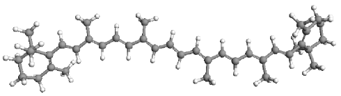
Figure 6: s-cis $\beta$-carotene.

Carotenoids, the family of substituted polyenes, are the primary light harvesting pigments in the LH2 complex. Light harvesting proceeds by the transfer of energy from an array of carotenoids to nearby bacteriochlorophylls and thence to the photosynthetic centre. Many essential questions remain unanswered as to the precise mechanism of this energy transfer sunstrom1 ; schulten-carotene ; fleming ; hsuhead-gordon1 ; hsuhead-gordon ; dreuw-carotene ; dreuw2003cfq . While the absorption of light places the carotenoid in the dipole allowed excited state, there can be a fast internal conversion to the aforementioned dark states of the polyene backbone, and thus multiple pathways for energy transfer to the bacteriochlorophyll. In carotenoids, the dipole allowed transition is usually labelled $S2$, while historically the dark state is labelled $S1$. However, with the discovery, as previously described, of additional dark states below $S2$ in these molecules cogdellscience ; onaka ; sashima ; sashima2 ; furuichi ; fujii , this nomenclature can be confusing. An alternative nomenclature is to simply re-use the polyene excited state labels, even though the carotenoids have a lower point group symmetry. We will follow this practice here.

III.2.1 Discussion

Table 3: DMRG-CASSCF energies, symmetries, and oscillator strengths for the lowest lying singlet excited states in $\beta$-carotene with the complete $\pi$-valence (22,22) active space. Total energies in $E_{h}$, excitation energies in $eV$, oscillator strengths in $a.u.$. The estimated error of the DMRG-CASSCF energies from the exact CASSCF energies in the same active space is less than 0.1m$E_{h}$. Oscillator strengths are for the ground-state, excited state transition.

Symmetry	DMRG-CASSCF	Excitation	Oscillator	Expt
	total energy	energy	Strength
$1A_{g}^{-}$	$-1546.914545$
$2A_{g}^{-}$	$-1546.804503$	$2.99$	Forbidden	$1.81$
$1B_{u}^{-}$	$-1546.781125$	$3.63$	$0.2025$	$2.05$
$3A_{g}^{-}$	$-1546.755822$	$4.31$	Forbidden	$(2.22)$

Figure 7: Polyene and carotene excitation energies vs the number of double bonds: the $\beta$-carotene excitation energies when fitted to the polyene excitation energies give an effective conjugation length of $9.5-9.7$.

(a) LUMO+1 natural orbital

(b) LUMO natural orbital

(c) HOMO natural orbital

(d) HOMO-1 natural orbital

Figure 8: Natural orbitals corresponding to the HOMO-1 through LUMO+1 states.
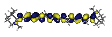
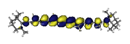
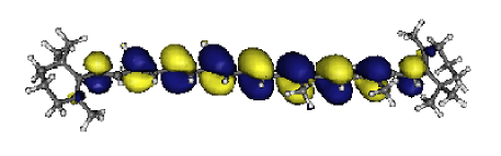
These orbitals participate in the lowest lying singlet excitations in $\beta$-carotene and contain little density on the non-planar end groups.

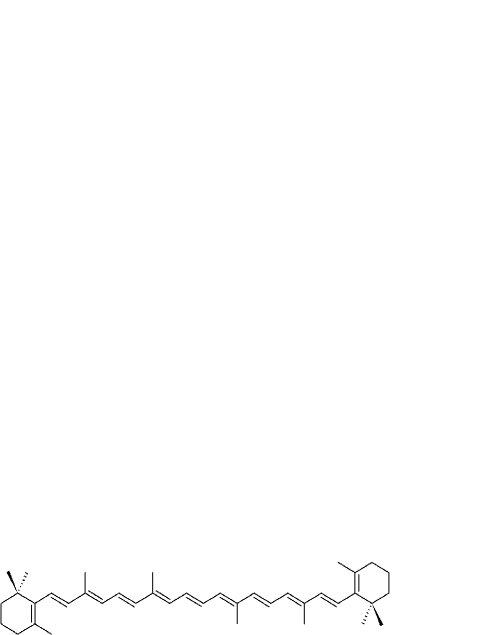
We have chosen to study s-cis $\beta$-carotene (see Fig. 6) as a representative carotenoid. It is the dominant natural conformer although the all-trans form is also studied. Crystalline $\beta$-carotene has $C_{i}$ symmetry with a conjugated backbone that lies almost entirely on the $xy$ plane except for end groups which are twisted out of plane Schlucker772 ; Berezin771 . (In the biological setting, carotenoid pigments usually adopt a twisted configuration in the conjugated backboneWang770 ; Qian757 ). There are 11 conjugated double bonds in the backbone. Our study employed the same calculation procedure as described in Sec. III.1.2 with the exception that we used a 6-31G basis set in the DMRG-CASSCF calculation due to the large size of the molecule. State-averaged DMRG-CASSCF calculations were performed with 4 states and a (22,22) complete $\pi$-valence space, in the manner described in Sec. III.1.2.

In Table 3 we present the energies, symmetries, and oscillator strengths for the ground state and first 3 excitations in $\beta$-carotene. We reproduce the state ordering $1A_{g}^{-}<2A_{g}^{-}<1B_{u}^{-}<3A_{g}^{-}$ as assigned by Furuichi et al. furuichi (note that the $1B_{u}^{+}$ which does not appear in our calculation indeed lies above the $3A_{g}^{-}$ state in this molecule). However, just as in the polyenes, the excitation energies from the DMRG-CASSCF procedure are generally overestimated in comparison with experiment, most likely due to the lack of $\sigma$-$\pi$ dynamic correlation.

A question that has received some attention in the literature is the effective conjugation length of carotenoids, since the presence of substituents and non-planar geometries are expected to modify this from the naive value deduced from the Lewis structure frankscites . Formally, $\beta$-carotene has 11 double bonds in the polyene backbone, but by comparing the excitation energies of the polyenes with our $\beta$-carotene excitation energies, we can estimate a reduced conjugation length of 9.5-9.7 bonds, which is very close to the experimental estimate of 9.7 of Onaka et al. onaka . This reduced conjugation length results from the twist in the carotene end-groups. In Fig. 8 we plot the DMRG-CASSCF natural orbitals corresponding to the HOMO, HOMO-1, LUMO, and LUMO+1. As can be seen, there is very little density in these orbitals on the carotene end-groups, and this is consistent with our reduced effective conjugation length.

IV Conclusion

In this work, we described how to efficiently implement orbital optimisation using the Density Matrix Renormalization Group (DMRG) wavefunction. We have named the resulting method DMRG-CASSCF, and by virtue of the compact nature of the DMRG wavefunction, this now enables us to handle much larger active spaces than are possible with the traditional CASSCF algorithm. As a sample application, we have used our DMRG-CASSCF implementation to study the low-lying excitations of polyenes from $\text{C}_{8}\text{H}_{10}$ to $\text{C}_{24}\text{H}_{26}$ as well as the light-harvesting pigment $\beta$-carotene, with up to a (24,24) complete active space. Our calculations reproduce the state ordering of the dark states that have been recently observed by Resonance Raman studies. However, as expected from earlier CASSCF studies, the energy of the optically allowed HOMO-LUMO $1B_{u}^{+}$ transition is still overestimated, as a result of the lack of dynamic $\sigma$-$\pi$ correlation in the DMRG-CASSCF method. We therefore view the incorporation of dynamic correlation, either via perturbation theory or via canonical transformation whitecd ; yanaict1 into the DMRG-CASSCF method to present an important next direction for development.

V Acknowledgments

This work was supported by Cornell University, the Cornell Center for Materials Research (CCMR), the David and Lucile Packard Foundation, the National Science Foundation CAREER program CHE-0645380, the Alfred P. Sloan Foundation, and the Department of Energy, Office of Science through award DE-FG02-07ER46432. Johannes Hachmann would like to acknowledge support provided by a Kekulé Fellowship of the Fond der Chemischen Industrie.

References

- (1) S. R. White, Phys. Rev. Lett. 69, 2863 (1992).
- (2) S. R. White, Phys. Rev. B 48, 10345 (1993).
- (3) S. R. White and R. L. Martin, J. Chem. Phys. 110, 4127 (1999).
- (4) A. O. Mitrushenkov, G. Fano, F. Ortolani, R. Linguerri, and P. Palmieri, J. Chem. Phys. 115, 6815 (2001).
- (5) G. K.-L. Chan and M. Head-Gordon, J. Chem. Phys. 116, 4462 (2002).
- (6) Ö. Legeza, J. Röder, and B. A. Hess, Phys. Rev. B 67, 125114 (2003).
- (7) G. Moritz and M. Reiher, J. Chem. Phys. 126, 244109 (2007).
- (8) G. K.-L. Chan and M. Head-Gordon, J. Chem. Phys. 118, 8551 (2003).
- (9) G. K.-L. Chan, M. Kállay, and J. Gauss, J. Chem. Phys. 121, 6110 (2004).
- (10) J. Hachmann, W. Cardoen, and G. K.-L. Chan, J. Chem. Phys. 125, 144101 (2006).
- (11) J. J. Dorando, J. Hachmann, and G. K.-L. Chan, J. Chem. Phys. 127, 084109 (2007).
- (12) J. Hachmann, J. J. Dorando, M. Avilés, and G. K.-L. Chan, J. Chem. Phys. 127, 134309 (2007).
- (13) S. Daul, I. Ciofini, C. Daul, and S. R. White, Int. J. Quantum Chem. 79, 331 (2000).
- (14) J. Rissler, R. M. Noack, and S. R. White, Chem. Phys. 323, 519 (2006).
- (15) A. O. Mitrushenkov, R. Linguerri, P. Palmieri, and G. Fano, J. Chem. Phys. 119, 4148 (2003).
- (16) A. O. Mitrushenkov, G. Fano, R. Linguerri, and P. Palmieri, arXiv:cond-mat 0306058v1 (2003).
- (17) G. K.-L. Chan, J. Chem. Phys. 120, 3172 (2004).
- (18) G. K.-L. Chan and T. Van Voorhis, J. Chem. Phys. 122, 204101 (2005).
- (19) Ö. Legeza and J. Sólyom, Phys. Rev. B 68, 195116 (2003).
- (20) Ö. Legeza, J. Röder, and B. A. Hess, Mol. Phys. 101, 2019 (2003).
- (21) Ö. Legeza and J. Sólyom, Phys. Rev. B 70, 205118 (2004).
- (22) G. Moritz, B. A. Hess, and M. Reiher, J. Chem. Phys. 122, 024107 (2005).
- (23) G. Moritz, A. Wolf, and M. Reiher, J. Chem. Phys. 123, 184105 (2005).
- (24) G. Moritz and M. Reiher, J. Chem. Phys. 124, 034103 (2006).
- (25) D. Zgid and M. Nooijen, J. Chem. Phys. , in press.
- (26) S. Ramasesha, S. K. Pati, H. R. Krishnamurthy, Z. Shuai, and J. L. Brédas, Synth. Met. 85, 1019 (1997).
- (27) D. Yaron, E. E. Moore, Z. Shuai, and J. L. Brédas, J. Chem. Phys. 108, 7451 (1998).
- (28) Z. Shuai, J. L. Brédas, A. Saxena, and A. R. Bishop, J. Chem. Phys. 109, 2549 (1998).
- (29) G. Fano, F. Ortolani, and L. Ziosi, J. Chem. Phys. 108, 9246 (1998).
- (30) G. L. Bendazzoli, S. Evangelisti, G. Fano, F. Ortolani, and L. Ziosi, J. Chem. Phys. 110, 1277 (1999).
- (31) C. Raghu, Y. Anusooya Pati, and S. Ramasesha, Phys. Rev. B 65, 155204 (2002).
- (32) C. Raghu, Y. Anusooya Pati, and S. Ramasesha, Phys. Rev. B 66, 035116 (2002).
- (33) F. Verstraete, D. Porras, and J. I. Cirac, Phys. Rev. Lett. 93, 227205 (2004).
- (34) F. Verstraete and J. I. Cirac, arXiv:cond-mat 0407066v1 (2004).
- (35) D. Pérez-Garciá, F. Verstraete, J. I. Cirac, and M. M. Wolf, arXiv:quant-ph 0707.2260v1 (2007).
- (36) N. Schuch, M. M. Wolf, F. Verstraete, and J. I. Cirac, Phys. Rev. Lett. 98, 140506 (2007).
- (37) V. Murg, F. Verstraete, and J. I. Cirac, Phys. Rev. A 75, 033605 (2007).
- (38) G. Vidal, arXiv:quant-ph 0610099v1 (2006).
- (39) J. Matos, B. O. Roos, and P. Malmqvist, J. Chem. Phys. 86, 1458 (1987).
- (40) B. O. Roos, Adv. Chem. Phys. 69, 339 (1987).
- (41) K.Nakayama, H. Nakano, and K.Hirao, Int. J. Quantum Chem. 66, 157 (1998).
- (42) Y. Kurashige, H. Nakano, Y.Nakao, and K. Hirao, Chem. Phys. Lett. 400, 425 (2004).
- (43) P. Knowles and H. Werner, J. Chem. Phys. 82, 5053 (1985).
- (44) D. Yeager, D. Lynch, J. Nichols, P. Jørgensen, and J. Olsen, J. Phys. Chem. 86, 2140 (1982).
- (45) G. K.-L. Chan, J. Dorando, D. Ghosh, J. Hachmann, E. Neuscamman, H. Wang, and T. Yanai, arXiv:cond-mat 0711.1398v1 (2007).
- (46) U. Schollwöck, Rev. Mod. Phys. 77, 259 (2005).
- (47) M. Fannes, B. Nachtergaele, and R. F. Werner, Comm. Math. Phys. 144, 443 (1992).
- (48) S. Östlund and S. Rommer, Phys. Rev. Lett. 75, 3537 (1995).
- (49) S. Rommer and S. Östlund, Phys. Rev. B 55, 2164 (1997).
- (50) B. Lengsfield III and B. Liu, J. Chem. Phys. 75, 478 (1981).
- (51) J. Pipek and P. Mezey, J. Chem. Phys. 90, 4916 (1989).
- (52) R. Pariser, J. Chem. Phys. 24, 250 (1956).
- (53) J. Hubbard, Proc. R. Soc. London, Ser. A 276, 238 (1963).
- (54) S. Ramasesha, S. Pati, H.R.Krishnamurthy, Z. Shuai, and J. Brédas, Phys. Rev. B 54, 7598 (1996).
- (55) P. Tavan and K. Schulten, J. Chem. Phys. 85, 6602 (1986).
- (56) M. Aoyagi, I. Ohmine, and B. Kohler, J. Chem. Phys. 94, 3922 (1990).
- (57) B. Hudson and B. Kohler, J. Chem. Phys. 14, 299 (1973).
- (58) L. Serrano-Andrés, J. Sanchez-Mańn, and I. Nebot-Gil, J. Chem. Phys. 97, 7499 (1992).
- (59) R. Cave, J. Chem. Phys. 92, 2450 (1990).
- (60) B. Brooks and H. Schaefer III, J. Chem. Phys. 68, 4839 (1978).
- (61) C. Petrongolo, R. Buenker, and S. Peyerimhoff, J. Chem. Phys. 76, 3655 (1982).
- (62) J. Lappe and R. Cave, J. Chem. Phys. 104, 2294 (2000).
- (63) A. Lasaga, R. Aerni, and M. Karplus, J. Chem. Phys. 73, 5230 (1980).
- (64) V. Bachler and K. Schaffner, Chem. Eur. J. 6, 959 (2000).
- (65) R. Hosteny, T. Dunning Jr, R. Gilman, A. Pipano, and I. Shavitt, J. Chem. Phys. 62, 4764 (1975).
- (66) R. Cave and E. Davidson, J. Phys. Chem. 92, 614 (1988).
- (67) T. Sashima, H. Nagae, M. Kuki, and Y. Koyama, Chem. Phys. Lett. 299, 187 (1999).
- (68) T. Sashima, Y. Koyama, T. Yamada, and H. Hashimoto, J. Phys. Chem. B 104, 5011 (2000).
- (69) R. Fujii, T. Ishikawa, Y. Koyama, M. Taguchi, Y. Isobe, H. Nagae, and Y. Watanabe, J. Phys. Chem. A 105, 5348 (2001).
- (70) K. Onaka, R. Fujii, H. Nagae, M. Kuki, Y. Koyama, and Y. Watanabe, Chem. Phys. Lett. 315, 75 (1999).
- (71) K. Furuichi, T. Sashima, and Y. Koyama, Chem. Phys. Lett. 356, 547 (2002).
- (72) G. Cerullo, D. Polli, G. Lanzani, S. D. Silvestri, H. Hashimoto, and R. Cogdell, Science 298, 2395 (2002).
- (73) A. D. Becke, J. Chem. Phys. 98, 5648 (1993).
- (74) C. Lee, W. Yang, and R. G. Parr, Phys. Rev. B 37, 785 (1988).
- (75) M. J. Frisch et al., Gaussian 03, Revision C.02, Gaussian, Inc., Wallingford CT, 2004, see http://www.gaussian.com/.
- (76) T. Dunning Jr, J. Chem.Phys. 90, 1007 (1989).
- (77) T. D. Crawford, C. D. Sherrill, E. F. Valeev, J. T. Fermann, R. A. King, M. L. Leininger, S. T. Brown, C. L. Janssen, E. T. Seidl, J. P. Kenny, and W. D. Allen, Psi 3.2 (2003), see www.psicode.org.
- (78) T. D. Crawford et al., J. Comput. Chem. 28, 1610 (2007).
- (79) S.R.White, Phys. Rev. B. 72, 180403 (2005).
- (80) M. Granville, G. Holtom, B. Kohler, R. Christensen, and K. D’Amico, J. Chem. Phys. 70, 593 (1979).
- (81) B. Kohler, C. Spangler, and C. Westerfield, J. Chem. Phys. 89, 5422 (1988).
- (82) L. Serrano-Andrés, M. Merchán, I. Nebot-Gil, R. Lindh, and B. O. Roos, J. Chem. Phys. 98, 3151 (1993).
- (83) R. Lindh and B. O. Roos, Int. J. Quantum Chem. XXXV, 813 (1989).
- (84) K. Hirao, Chem. Phys. Lett. 190, 374 (1992).
- (85) P. Tavan and K. Schulten, Phys. Rev. B 36, 4337 (1987).
- (86) A. Dreuw, G. Fleming, and M. Head-Gordon, Phys. Chem. Chem. Phys. 5, 3247 (2003).
- (87) V. Sundström, Progress in Quantum Electronics 24, 187 (2000).
- (88) A. Damjanovic, T. Ritz, and K. Schulten, Phys. Rev. E 59, 3293 (1999).
- (89) P. Walla, P. Linden, C.-P. Hsu, G. Scholes, and G. Fleming, Proc. Nat. Acad. Sci. 97, 10808 (2000).
- (90) C.-P. Hsu, P. Walla, M. Head-Gordon, and G. Fleming, J. Phys. Chem. B 105, 11016 (2001).
- (91) C.-P. Hsu, S. Hirata, and M. Head-Gordon, J. Phys. Chem. A 105, 451 (2001).
- (92) A. Dreuw, G. Fleming, and M. Head-Gordon, Phys. Chem. Chem. Phys. 5, 3247 (2003).
- (93) S. Schlücker, A. Szeghalmi, M. Schmitt, J. Popp, and W. Kiefer, Journal of Raman Spectroscopy 34, 413 (2003).
- (94) K. V. Berezin and V. V. Nechaev, Journal of Applied Spectroscopy 72, 164 (2005).
- (95) Y. Wang, L. Mao, and X. Hu, Biophysical Journal 86, 3097 (2004).
- (96) P. Qian, K. Saiki, T. Mizoguchi, K. Hara, T. Sashima, R. Fujii, and Y. Koyama, Photochemistry and Photobiology 74, 444 (2001).
- (97) H. Frank, Archives of Biochemistry and Biophysics 385, 53 (2001).
- (98) T. Yanai and G. K.-L. Chan, J. Chem. Phys. 124, 194106 (2006).
- (99) S. R. White, J. Chem. Phys. 117, 7472 (2002).