Correlation between the transition temperature and the superfluid density in BCS superconductor NbB_2+x

Abstract

The results of the muon-spin rotation experiments on BCS superconductors NbB_2+x ($x=0.2$, 0.34) are reported. Both samples, studied in the present work, exhibit rather broad transitions to the superconducting state, suggesting a distribution of the volume fractions with different transition temperatures ($T_{c}$)’s. By taking these distributions into account, the dependence of the inverse squared zero-temperature magnetic penetration depth ($\lambda_{0}^{-2}$) on $T_{c}$ was reconstructed for temperatures in the range $1.5$ K$\lesssim T_{c}\lesssim 8.0$ K. $\lambda_{0}^{-2}$ was found to obey the power law dependence $\lambda_{0}^{-2}\propto T_{c}^{3.1(1)}$ which appears to be common for some families of BCS superconductors as, e.g., Al doped MgB₂ and high-temperature cuprate superconductors as underdoped YBa₂Cu₃O_7-δ.

I Introduction

The search for universal correlations between physical variables, such as transition temperature, magnetic field penetration depth, electrical conductivity, energy gap, Fermi energy etc. may provide hints towards a unique classification of different superconductors. In particular, establishing of such correlations may help to understand the phenomenon of superconductivity, that is observed now in quite different systems, such as simple metals and alloys, fullerenes, molecular metals, cuprates, cobaltites, borides etc. Among others, there is a correlation between the transition temperature ($T_{c}$) and the inverse squared zero-temperature magnetic field penetration depth ($\lambda_{0}^{-2}$), that generally relates to the zero-temperature superfluid density ($\rho_{s}$) in terms of $\rho_{s}\propto\lambda_{0}^{-2}$. In various families of underdoped high-temperature cuprate superconductors (HTS)’s there is the empirical relation $T_{c}\propto\rho_{s}\propto\lambda_{0}^{-2}$, first identified by Uemura et al.Uemura89 ; Uemura91 It was recently shown, however, that for HTS’s with highly reduced $T_{c}$’s the direct proportionality between $T_{c}$ and $\lambda_{0}^{-2}$ is changed to a power law kind of dependence with $(T_{c})^{n}\propto\lambda_{0}^{-2}$ ($n$ is the power law exponent). In experiments on highly underdoped YBa₂Cu₃O_7-δ Zuev et al.Zuev05 obtained $n=2.3$, Liang and coworkers reported $n=1.6$,Liang05 while Sonier et al.Sonier07 found $n=2.6-3.1$. In molecular superconductors Pratt and Blundell obtained $n=2/3$.Pratt05 From the theoretical point of view, it was shown that in systems obeying 2D or 3D quantum superconductor to insulator transition, $n\equiv 1$ or $n\equiv 2$, respectively.Kim91 ; Schneider00 ; Schneider04 ; Schneider07

It should be emphasized, however, that the relation between $T_{c}$ and $\lambda_{0}^{-2}$ is not yet established for BCS superconductors and still awaits to be explored. A good candidate to search for such a relation could be NbB_2+x. The superconductivity in NbB_2+x, similar to MgB₂, is most likely mediated by phonons. It is confirmed in nuclear magnetic resonance (NMR)Kotegawa02 and tunnelling experiments,Takasaki04 ; Ekino04 as well as by recent calculations of the elastic properties.Regalado07 Moreover, muon-spin rotation ($\mu$SR) experiments suggest that the superconducting gap is isotropic.Takagiwa04 As is shown in Refs. Escamilla04, and Yamamoto01, the superconductivity in NbB₂ can be induced by either increasing boron or decreasing niobium content, while the parent NbB₂ compound is not superconducting at least down to 2 K. The transition temperature was found to reach the maximum value of $9.2$ K and $9.8$ K for Nb_0.9B₂ and NbB_2.34, respectively.Escamilla04 ; Yamamoto01 This offers a possibility to study the relation between $T_{c}$ and $\lambda_{0}^{-2}$ as a function of boron and/or niobium content. In the present study the temperature dependence of the magnetic field penetration depth was measured for two NbB_2+x samples with $x=0,2$ and 0.34 by means of transverse-field muon-spin rotation technique. It was found that in both samples the distribution of the superconducting volume fractions with different $T_{c}$’s can be well approximated by a Gaussian distribution. The mean values of the superconducting transition temperature ($T^{m}_{c}$) and the width of the distribution ($\Delta T_{c}$) were found to be $T^{m}_{c}=6.02(3)$ K, $\Delta T_{c}=0.96(2)$ K for NbB_2.34 at $\mu_{0}H=0.1$ T, and $T^{m}_{c}=3.40(4)$ K, $\Delta T_{c}=1.06(2)$ K for NbB_2.2 at $\mu_{0}H=0.05$ T. Within the model, developed for a granular superconductor of moderate quality, we reconstruct the dependence of the zero-temperature superfluid density $\rho_{s}\propto\lambda_{0}^{-2}$ on the transition temperature $T_{c}$. It was found that in the range of $1.5$ K$\lesssim T_{c}\lesssim 8.0$ K $\lambda_{0}^{-2}$ follows a power law dependence, rather than a linear dependence reported by Takagiwa et al.,Takagiwa04 with $\lambda_{0}^{-2}\propto T_{c}^{3.1(1)}$. The value of the power law exponent 3.1(1) agrees rather well with $n=2.6-3.1$ reported by Sonier et al.Sonier07 for underdoped HTS’s YBa₂Cu₃O_7-δ.

The paper is organized as follows. In Sec. II.1 we describe the model used to obtain the temperature dependence of the magnetic field penetration depth for a granular superconductor having a certain distribution of the superconducting volume fractions. The distributions of the local magnetic fields, calculated within the framework of this model, are presented in Sec. II.2. In Sec. III we describe the sample preparation procedure and details of the muon-spin rotation and magnetization experiments. Sec. IV comprises studies of the magnetic penetration depth in NbB_2.2 and NbB_2.34 superconductors. The conclusions follow in Section V.

II Theoretical background

II.1 Magnetic penetration depth in a granular superconductor of moderate quality

In this section we describe the model applied to calculate temperature dependence of the magnetic field penetration depth $\lambda$ in a granular superconductor of moderate quality by using the $\mu$SR data. We based on a general assumption that $\lambda$ can be obtained from the second moment of the local magnetic field distribution [$P(B)$] inside the superconducting sample in the mixed state measured directly in $\mu$SR experiments . The model uses following assumptions: (i) The superconducting grains are decoupled from each other. (ii) Each $i-$th grain is a superconductor with a certain value of the transition temperature ($T^{i}_{c}$) and the zero-temperature magnetic penetration depth ($\lambda^{i}_{0}$). (iii) The zero-temperature superconducting gap ($\Delta_{0}$) scales with $T_{c}$ in agreement with the well-known relation $\Delta_{0}/k_{B}T_{c}=const$,Tinkham75 implying that the ratio $R=\Delta_{0}^{i}/k_{B}T_{c}^{i}$ is the same for all the grains. Note that a linear decrease of both superconducting energy gaps ($\Delta^{\sigma}$ and $\Delta^{\pi}$) with decreasing $T_{c}$ was observed recently by Gonelli et al.Gonnelli06 in Mn doped MgB₂. The similar linear $\Delta_{0}$ vs. $T_{c}$ scaling was reported by Khasanov et al.Khasanov04 for RbOs₂O₆ BCS superconductor.

Let us first define variables and functions used within the model. Function $\omega(t)$ describes the distribution of the superconducting volume fractions with different transition temperatures $T_{c}$’s. It is defined so that the volume fraction of the sample, having transition temperatures in the range between $T_{c}^{i}$ and $T_{c}^{j}$, is obtained as $\int_{T_{c}^{i}}^{T_{c}^{j}}\omega(t)dt$. The distribution of the local magnetic fields in the $i-$th grain is described by the function $P^{i}(B)$, which for ideal superconductor has rather asymmetric shape [see Fig. 1 (a)]. Function $f(t)$ describes dependence of the inverse squared magnetic penetration depth $\lambda^{-2}$ at $T=0$ on $T_{c}$ [$(\lambda_{0}^{i})^{-2}=f(T_{c}^{i})$]. The dependence of $\lambda^{i}$ on temperature was assumed to follow the standard equation for weak coupled BCS superconductor [see, e.g., Eq. (2-111) in Ref. Tinkham75, ]:

$$[\lambda^{i}(T)]^{-2}=(\lambda^{i}_{0})^{-2}s(T,\Delta_{0}^{i})=f(T_{c}^{i})s(T,k_{B}R\cdot T_{c}^{i}),$$ (1)

with the temperature dependent part

$$s(T,\Delta_{0}^{i})=1+2\int_{\Delta^{i}(T)}^{\infty}\left(\frac{\partial F}{\partial E}\right)\frac{E}{\sqrt{E^{2}-\Delta^{i}(T)^{2}}}\ dE.$$

Here, $F=[1+\exp(E/k_{B}T)]^{-1}$ is the Fermi function, $\Delta^{i}(T)=\Delta_{0}^{i}\tilde{\Delta}(T/T_{c}^{i})$ represents the temperature dependence of the energy gap, and $\Delta^{i}_{0}=2Rk_{B}T_{c}^{i}$ denotes the zero temperature value of the superconducting gap. For the normalized gap $\tilde{\Delta}(T/T_{c})$ the values tabulated in Ref. Muhlschlegel59, were used. Finally, the temperature dependence of the total second moment of the local magnetic field distribution in the superconducting sample can obtained as:

$$\langle\Delta B^{2}\rangle^{tot}=\frac{\sigma^{2}}{\gamma_{\mu}^{2}}=\int_{T}^{\infty}\int_{0}^{\infty}\omega(t)P(B^{\prime},t)(B^{\prime}-B^{m})^{2}dtdB^{\prime}.$$ (2)

Here, $\gamma_{\mu}=2\pi\times 135.5342$ MHz/T is the muon gyromagnetic ratio, $\sigma^{2}$ is the second moment of the $\mu$SR line and $B^{m}$ is the mean internal field inside the superconducting sample.

As will be shown later, in transverse-field $\mu$SR experiments one obtains directly: (i) the distribution of the superconducting volume fractions with different $T_{c}$’s [$\omega(T_{c})$], (ii) the temperature dependence of the mean internal field $B^{m}(T)$, and (iii) the temperature dependence of the second moment of the $\mu$SR line $\sigma^{2}(T)$. By substituting $\omega(T_{c})$ and $B^{m}(T)$ to the Eq. (2) and then fitting it to the experimental $\sigma(T)$ data, one should be able to obtain the distribution of the zero-temperature superfluid density $\rho_{s}\propto\lambda_{0}^{-2}$ as a function of the transition temperature $T_{c}$ and the ratio $R=\Delta_{0}/k_{B}T_{c}$. In order to do that one needs, however, to calculate $P^{i}(B)$ distributions which depend on the applied field ($B_{ex}$), $\lambda^{i}$, and the coherence length ($\xi^{i}$) in a nontrivial way. This makes fit of Eq. (2) to the experimental data extremely difficult. The analysis can be simplified by assuming that each $P^{i}(B)$ follows the Gaussian distribution and is determined, therefore, by the only two parameters: the second moment of the Gaussian line

$$\langle\Delta B^{2}\rangle=(\sigma/\gamma_{\mu})^{2}=G^{2}(b)\cdot(\lambda)^{-4},$$

and the internal field of the $i-$th grain ($B^{i}$). Here, $b=B/B_{c2}$ is the reduced magnetic field ($B_{c2}$ is the second critical field) and the $G(b)$ is the proportionality coefficient between $\sigma/\gamma_{\mu}=\sqrt{\langle\Delta B^{2}\rangle}$ and $\lambda^{-2}$ which can be obtained by means of Eq. (13) from Ref. Brandt03, as:

$$G(b)=0.172\frac{\Phi_{0}}{2\pi}(1-b)[1+1.21(1-\sqrt{b})^{3}],$$ (3)

($\Phi_{0}$ is the magnetic flux quantum). Here we also take into account that within Ginzburg-Landau theory $\xi=\sqrt{\Phi_{0}/2\pi B_{c2}}$. The internal field of the $i-$th grain was calculated within the London approximation modified by Brandt:Brandt03

$$B^{i} = B_{ex}-(1-D^{i})\frac{\Phi_{0}}{8\pi\cdot(\lambda^{i})^{2}}\ln[g(b^{i})]$$ (4)

$$\simeq B_{ex}-(1-D^{m})\frac{\Phi_{0}}{8\pi}f(T_{c}^{i})s(T,k_{B}RT_{c}^{i})\ln[g(b^{m})]$$

where

$$g(b)=1+\frac{1-b}{b}(0.357+2.890b-1.581b^{2}),$$

$b^{i}=B^{i}/B^{i}_{c2}$, and $b^{m}=B^{m}/B^{m}_{c2}$. $B^{i}_{c2}$ and $D^{i}$ are the second critical field and the demagnetization factor of the $i-$th grain, and $D^{m}$ and $B^{m}_{c2}$ are the mean values of the demagnetization factor and the second critical field, respectively. In the last part of Eq. (4), we also replaced $D^{i}$ and $b^{i}$ by their average values $D^{m}$ and $b^{m}$ (it is clear, that in the intermediate range of fields and for temperatures not very close to $T_{c}$, $b^{i}\simeq b^{m}$).

The advantage to use Gaussian $P^{i}(B)$ is that the contribution of the $i-$th line to the total second moment can be obtained analytically as:Weber93 ; Khasanov05-RbOs

$$\langle\Delta B^{2}\rangle^{i} = (\sigma^{i}/\gamma_{\mu})^{2}+(B^{i}-B^{m})^{2}\simeq$$ (5)

$$G^{2}(b^{m})[\lambda^{i}(T)]^{-4}+(B^{i}-B^{m})^{2}.$$

By substituting it in Eq. (2) one gets:

$$\langle\Delta B^{2}\rangle^{tot}=\frac{\sigma^{2}}{\gamma_{\mu}^{2}}=\int_{T}^{\infty}\omega(t)\langle\Delta B^{2}\rangle dt.$$ (6)

Later on we are going to use this equation in order to fit the experimental $\mu$SR data. We want to remind that the total second moment $\langle\Delta B^{2}\rangle^{tot}$ obtained by means of Eq. (6) is determined by: (i) Function $f(T_{c})$ that describes distribution of $\lambda_{0}^{-2}$ as a function of $T_{c}$ [see Eq. (1)]. (ii) Function $\omega(T_{c})$ describing distribution of the superconducting fractions with different $T_{c}$’s. (iii) Gap to $T_{c}$ ratio $R=2\Delta_{0}/k_{B}T_{c}$ [see Eq. (1)]. (iv) The mean values of the demagnetization factor $D^{m}$ and the reduced magnetic field $b^{m}$ [see Eq. (4) and (5)].

Note that in real experiments on polycrystalline samples with sharp transition to the superconducting state, $P(B)$ often obeys Gaussian distribution (see, e.g., Refs. Weber93, and Pumpin90, ). The reason is that the vortex lattice within the small superconducting grain does not remain regular. It is distorted due to effects of pinning inside the grain, as well as, near the edges of the grain due to closeness of vortexes to the surface. As is shown by Brandt,Brandt88 even small pinning leads to substantial smearing of the characteristic features of the ideal $P(B)$ line and, in a case of intermediate pinning, to the Gaussian shape of $P(B)$. We should emphasize, however, that even in a case of distorted vortex lattice, the second moment of $P(B)$ is still a good measure of $\lambda$.Brandt88

II.2 Magnetic field distribution in a granular superconductor

In this section we are going to simulate the internal magnetic field distribution $P(B)$ within the above described model. As a first step it is necessary to choose a theoretical model describing the spatial variation of the local internal magnetic fields in the vortex lattice [$B({\bf r})$], from which the distribution of the fields in the $i-$th grain can be obtained as:

$$P^{i}(B)=\frac{\int\delta(B-B^{\prime})\ dA(B^{\prime})}{\int dA(B^{\prime})}.$$ (7)

Here, $dA(B^{\prime})$ is an elemental piece of the vortex lattice unit cell where the magnetic field is equal to $B^{\prime}$ and the unit cell has a total area of $\int dA(B^{\prime})$. $B({\bf r})$ was calculated by using an iterative method for solving the Ginzburg- Landau equations developed by Brandt.Brandt03 This method allows to accurately determine $B({\bf r})$ for arbitrary $b$, $\kappa=\lambda/\xi$ and the vortex lattice symmetry (see Refs. Brandt03, , Brandt97, , and Laulajainen06, for details).

Figure 1: (Color online) $P(B)$ distributions calculated by means of Eq. (10) at $T_{c}^{m}=6$ K, $\lambda_{0}(T_{c}^{m})=60$ nm, $\kappa=1.67$, and $B_{ex}=0.1$ T for the following values of $\Delta T_{c}$: 0.0 K (a) 0.2 K (b), 1.0 K (c), and 2 K (d). The dashed green, solid blue, and doted red lines in (b), (c), and (d) represent the $\omega(T_{c}^{i})P^{i}(B)$ term for $T_{c}^{i}=T_{c}^{m}-\Delta T_{c}$, $T_{c}^{i}=T_{c}^{m}$, and $T_{c}^{i}=T_{c}^{m}+\Delta T_{c}$, respectively. See text for details.

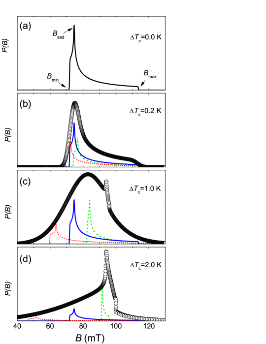
It was also assumed that the distribution of the superconducting volume fractions with different $T_{c}$’s is described by a Gaussian distribution:

$$\omega(T_{c}^{i})=\frac{1}{\Delta T_{c}\sqrt{2\pi}}\exp\left(-\frac{(T_{c}^{i}-T_{c}^{m})^{2}}{2\Delta T_{c}^{2}}\right)$$ (8)

($T^{m}_{c}$ and $\Delta T_{c}$ are the mean value and the width of the distribution, respectively), $\lambda_{0}^{-2}$ follows the power law:

$$\lambda_{0}^{-2}(T_{c}^{i})=(K\cdot T_{c}^{i})^{n}$$ (9)

with the exponent $n=2$, and $\kappa^{i}=\lambda^{i}/\xi^{i}=const$.comment As is mentioned already in the introduction, the power law dependence of $\lambda_{0}^{-2}$ on $T_{c}$ is observed for various HTSUemura89 ; Uemura91 ; Zuev05 ; Liang05 ; Sonier07 and molecular superconductors,Pratt05 as well as obtained theoretically for materials having 2D or 3D quantum superconductor to insulator transition.Kim91 ; Schneider00 ; Schneider04 ; Schneider07

As initial parameters for calculations we took $T_{c}^{m}=6$ K, $B_{ex}=0.1$ T, $D^{m}=1/3$, $\lambda_{0}(T_{c}^{m})=60$ nm and $\kappa=1.67$. The resulting field distribution $P(B)$ was obtained as:

$$P(B)=\sum_{i}^{N}\omega(T_{c}^{i})P^{i}(B).$$ (10)

Calculations were done for $N=60$ in the region $\pm 3\Delta T_{c}$ around $T_{c}^{m}$. Figure 1 shows $P(B)$ distributions for $\Delta T_{c}=0.0$ K, 0.2 K, 1.0 K and 2.0 K obtained by means of Eq. (10). The lines in (b), (c), and (d) represent the $\omega(T_{c}^{i})P^{i}(B)$ term for $T_{c}^{i}=T_{c}^{m}-\Delta T_{c}$ (dashed green line), $T_{c}^{i}=T_{c}^{m}$ (solid blue line), and $T_{c}^{i}=T_{c}^{m}+\Delta T_{c}$ (dotted red line). It is seen that the shape of $P(B)$ changes dramatically with increasing width of the $\omega(T_{c})$ distribution. For small $\Delta T_{c}$ (when transition to the superconducting state is very sharp) $P(B)$ is asymmetric with the highest weight around the point corresponding to the so called ”saddle point“ field $B_{sad}$ [see Figs. 1 (a) and (b)]. It is also seen that all the characteristic features of $P(B)$ at minimum ($B_{min}$), maximum ($B_{max}$), and ”saddle point“ fields are smeared out [see Fig. 1 (b)]. Note that the simulated $P(B)$ presented in Fig. 1 (b) looks very similar to what is observed in $\mu$SR experiments on high-quality single crystals.Herlach90 ; Sonier00 With a further increase of $\Delta T_{c}$ the $P(B)$ distribution becomes rather symmetric and, finally, asymmetric again, but now with the maximum weight around the external field $B_{ex}=0.1$ T and a very long tail at lower fields. It is interesting to note, that the parts of the sample with the lowest $T_{c}$’s are responsible for the peak appearing slightly below the external field, as is seen in Fig. 1 (c) and (d). The reason is the decrease of $P^{i}(B)$ width and the shift of $B^{i}$ towards to $B_{ex}$ with increasing $\lambda^{i}$.

To summarize, in Sec. II we described the model allowing to obtain the distribution of the internal magnetic fields in a granular superconducting sample of moderate quality and calculated the second moment of this distribution. Within the framework of this model we also simulated $P(B)$ profiles for materials with different width of the superconducting transition $\Delta T_{c}$. It is remarkable, that already small $\Delta T_{c}$ leads to smearing of the characteristic features of $P(B)$ distribution near $B_{min}$, $B_{sad}$, and $B_{max}$ characteristic fields. Even though this result is quite predictable, it has an important impact, since previously smearing of $P(B)$ was ascribed entirely for the effects of pinning (see, e.g., Ref. Sonier00, ).

III Experimental details

Figure 2: (Color online) Temperature dependences of the field-cooled magnetization ($M_{FC}$) for NbB_2.2 and NbB_2.34 samples measured at $\mu_{0}H=0.5$ mT. The solid lines are the best linear fits to the steepest part of $M_{FC}(T)$ curves and $M=0$.

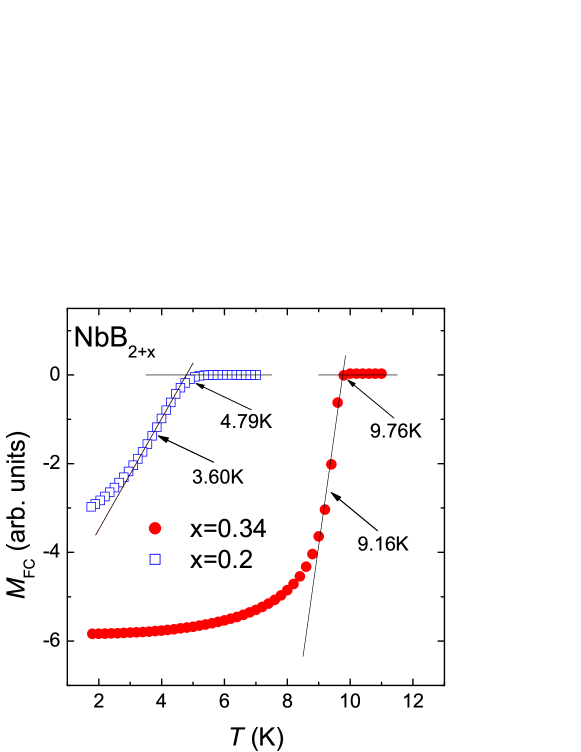
Details of the sample preparation for NbB_2+x can be found elsewhere Escamilla04 . Both NbB_2.2 and NbB_2.34 samples, studied in the present work, were fine powders with the average grain size of the order of few microns. The field-cooled 0.5 mT magnetization ($M_{FC}$) measurements for NbB_2.2 and NbB_2.34 samples were performed by using a SQUID magnetometer. The corresponding $M_{FC}(T)$ curves are shown in Fig. 2. It is seen that the superconducting transitions are rather broad indicating that both samples are not particularly uniform. This also implies that the superconducting critical temperatures may be evaluated only approximately. The middle-points of transitions correspond to $\simeq 9.16$ K and $\simeq 3.60$ K, while linear extrapolations of $M_{FC}(T)$ curves in the vicinity of $T_{c}$ to $M=0$ result in 9.76 K and 4.79 K for NbB_2.2 and NbB_2.34, respectively (see Fig. 2).

Figure 3: (Color online) The muon-time spectra (a), difference between the two-Gaussian fit and experimental data (b), and internal field distributions (c) for NbB_2.34 sample at $T=1.7$ K after field cooling in magnetic field of 0.1 T. The lines in (a) and (c) represent the best fit with the Gaussian line-shapes. See text for details.

The transverse-field $\mu$SR experiments were performed at the $\pi$M3 beam line at the Paul Scherrer Institute (Villigen, Switzerland). The powders of NbB_2.2 and NbB_2.34 were cold pressed into pellets (12 mm diameter and 2 mm thick). The samples were field cooled in $\mu_{0}H=0.05$ T (NbB_2.2) and 0.1 T (NbB_2.34), applied perpendicular to the flat surface of the pellet, from above $T_{c}$ down to 1.7 K. The fields 0.05 T and 0.1 T were chosen in order to perform measurements at the same reduced magnetic field $B/B_{c2}\simeq 0.4$ ($B_{c2}$ is the upper critical field).Khasanov06_unp The $\mu$SR signal was observed in the usual time-differential way by counting positrons from decaying muons as a function of time in positron telescopes. The time dependence of the positron rate is given by the expression:msr

$$\frac{{\rm d}N(t)}{{\rm d}t}=N_{0}{1\over\tau_{\mu}}e^{-t/\tau_{\mu}}\left[1+AP(t)\right]+bg\;,$$ (11)

where $N_{0}$ is the normalization constant, $bg$ denotes the time-independent background, $\tau_{\mu}=2.19703(4)\times 10^{-6}$ s is the muon lifetime, $A$ is the maximum decay asymmetry for the particular detector telescope ($A\simeq 0.18-0.19$ in our case), and $P(t)$ is the polarization of the muon ensemble:

$$P(t)=\int P(B)\cos(\gamma_{\mu}Bt+\phi)dB\;.$$ (12)

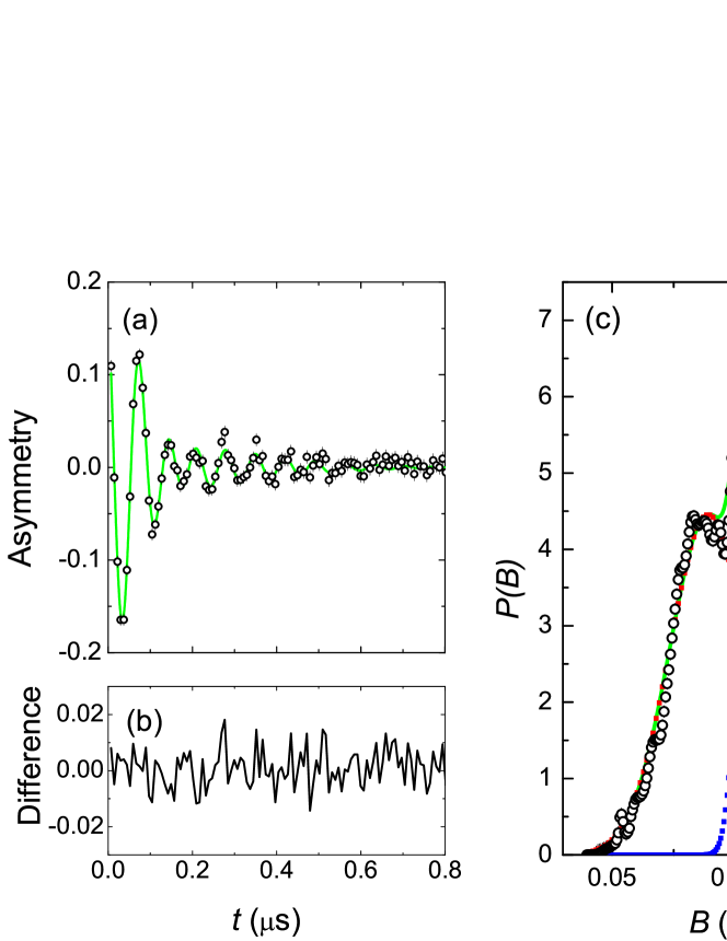
Here, $\phi$ is the angle between the initial muon polarization and the effective symmetry axis of a positron detector. $P(t)$ can be linked to the internal field distribution $P(B)$ by using the algorithm of Fourier transform.msr The $P(t)$ and $P(B)$ distributions inside the NbB_2.34 at $T=1.7$ K after field-cooling in a magnetic field of 0.1 T are shown in Fig. 3 (a) and (c). The $P(B)$ distributions were obtained from measured $P(t)$ by using the fast Fourier transform procedure based on the maximum entropy algorithm.Rainford94 In order to account for the field distribution seen in Fig. 3 (c), the $\mu$SR time-spectra were fitted by two Gaussian lines:

$$P(t)=\sum_{i=1}^{2}A_{i}\exp(-\sigma_{i}^{2}t^{2}/2)\cos(\gamma_{\mu}B_{i}t+\phi)\;.$$ (13)

where $A_{i}$, $\sigma_{i}$, and $B_{i}$ are the asymmetry, the Gaussian relaxation rate and the first moment of the $i$-th line. At $T\gtrsim 8$ K for NbB_2.34 and $T\gtrsim 4.5$ K for NbB_2.2 the analysis is simplified to the single line only with $\sigma_{nm}\simeq 0.3$ $\mu$s^-1 resulting from the nuclear moments of the sample. Eq. (13) is equivalent to the field distribution:Khasanov05-RbOs

$$P(B)=\gamma_{\mu}\sum_{i=1}^{2}{A_{i}\over\sigma_{i}}\exp\left(-{\gamma_{\mu}^{2}(B-B_{i})^{2}\over 2\sigma_{i}^{2}}\right)\;.$$ (14)

The solid line in Fig. 3 (a) represent the best fit with the two-Gaussian lines to the muon-time spectra. The corresponding $P(B)$ is shown in Fig. 3 (c). It should be mentioned that the two-Gaussian fit can satisfactory describe the experimental data. For both samples and in the whole range of temperatures the normalized $\chi^{2}_{\rm norm}$’s were found to be close to the unity implying a good quality of fits.

IV Results and discussions

Figure 4: (Color online) The temperature dependences of asymmetries ($A_{sc}$, $A_{n}$) (a)/(d), internal fields ($B_{sc}$, $B_{n}$) (b)/(e), and the muon-spin depolarization rates ($\sigma_{sc}$, $\sigma_{n}$) (c)/(f), obtained from the fit of $\mu$SR time spectra by means of Eq. (13) for NbB_2.34/NbB_2.2 after field-cooling in a magnetic field of 0.1 T/0.05 T. The indexes ”sc“ and ”n“ denote the normal and the superconducting state components. The dotted lines in (a)/(d) and (b)/(e) represent the total muon asymmetry ($A_{sc}+A_{n}$) and the external field value ($B_{ex}$), respectively. In the upper panels of (a) and (d) the $P(B)$ distributions at temperatures marked by the arrows are shown. The red and the blue dotted lines represent the superconducting (broad) and the normal state (narrow) components obtained from the fit by means of Eq. (13). The solid green line corresponds to the sum of these two components.

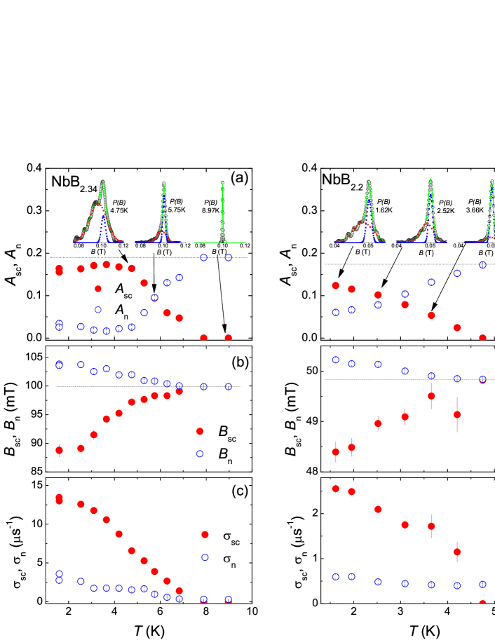
Results for NbB_2.2 and NbB_2.34, obtained from the fit of experimental data by means of Eq. (13), are summarized in Fig. 4. Distributions of the local fields, at temperatures marked by the arrows, are shown in the upper panels of Figs. 4 (a) and (d). The broad lines reflect contributions of the superconducting parts of samples. Indeed, their asymmetries $A_{sc}$ [Figs. 4 (a) and (d)] and relaxation rates $\sigma_{sc}$ [Figs. 4 (c) and (f)] increase while first moments $B_{sc}$ [Figs. (b) and (e)] decrease with decreasing temperature, as expected for a superconductor in a mixed state (see, e.g., Ref. Zimmermann95, ). The narrow lines describe contributions from parts of the samples being in the normal state. The slight shift of these lines to higher fields [Figs.  4 (b) and (e)] and the small increase of relaxations [Figs.  4 (c) and (f)] are associated with the diamagnetism of the superconducting grains leading to increase of the local fields in the nonsuperconducting parts of the sample. Such behavior is often observed in samples with less than 100% superconducting volume fraction (see, e.g., Refs. Khasanov05-RbOs, and Koda04, ).

In Fig. 5 we plot temperature dependences of the superconducting components $A_{sc}$ and $\sigma_{sc}$. The $\sigma_{sc}$ values presented in Fig. 5 are corrected to the nuclear moment contribution $\sigma_{nm}$ which was subtracted in quadrature (see e.g. Ref. Khasanov05-RbOs, ). It is seen [Fig. 5 (a)] that superconductivity does not disappear abruptly. The superconducting fraction decreases continuously from their maximum value to zero with temperature rising from 4 K to 8 K for NbB_2.34 and from 1.5 K to 5.5 K for NbB_2.2. The solid lines in Fig. 5 (a) correspond to fits of $A_{sc}(T)$, assuming that the distribution of the superconducting volume fractions with different $T_{c}$’s [$\omega(T_{c})$] follows the Gaussian distribution [see Eq. (8)] and, consequently,

$$A_{sc}(T)=A^{m}_{sc}\int_{T}^{\infty}\omega(t)dt\ .$$ (15)

Here, $A^{m}_{sc}$ is the mean value of the superconducting asymmetry at low temperatures. The fits yield $T^{m}_{c}$=6.02(3) K, $\Delta T_{c}$=0.96(2) K, and $A_{sc}^{m}$=0.170(5) for NbB_2.34, and $T^{m}_{c}$=3.40(4) K, $\Delta T_{c}$=1.06(2) K, and $A^{m}_{sc}$=0.128(7) for NbB_2.2. By taking into account that the total asymmetries ($A_{sc}+A_{n}$) were found to be $\simeq 0.19$ for NbB_2.34 and $\simeq 0.18$ for NbB_2.2 [dotted lines in Figs. 4(a) and (d)], the superconducting volume fractions were estimated to be $\simeq$85 % and $\simeq$70 % for NbB_2.34 and NbB_2.2, respectively.

Figure 5: (Color online) (a) Temperature dependences of the superconducting asymmetries ($A_{sc}$) for NbB_2.34 and NbB_2.2. The solid lines are the fits of $A_{sc}(T)$ data by means of Eq. (15). The dashed lines represents the Gaussian distributions of the superconducting volume fractions with different $T_{c}$’s [$\omega(T_{c})$]. (b) Temperature dependences of $\sigma_{sc}$ corrected to the nuclear moment contribution $\sigma_{nm}$ for NbB_2.34 and NbB_2.2. The open and filled small black circles are the fit of $\sigma_{sc}(T)$ by means of Eq. (6). See text for details.

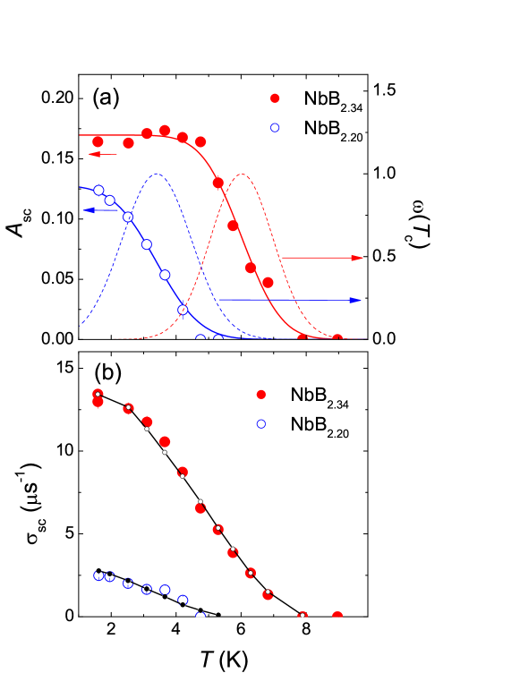
The samples used in our $\mu$SR experiments were cold pressed powders. In this case the individual grains are expected to be only weakly coupled. This implies that the model, described in Sec. II.1, can be applied for the particular NbB_2.2 and NbB_2.34 samples studied in the present work. All the variables and functions needed for such calculations as, e.g., the distribution of the superconducting volume fractions with different $T_{c}$’s [$\omega(T_{c})$ – dashed red and blue lines in Fig. 5 (a)], the temperature dependences of the square root of the second moment [$\sigma_{sc}(T)=\gamma_{\mu}\sqrt{\langle\Delta B^{2}\rangle(T)}$, see Figs. 4 (c) and (f)] and the mean field [$B_{sc}(T)=B^{m}(T)$, see Figs. 4 (b) and (e)] are directly obtained in the experiments. The only unknown parameter is the demagnetization factor $D^{m}$ which enters Eq. (4). We should mention, however, that it is not correct to assume that $D^{m}$ is equal to the some average demagnetization factor for all the grains as, e.g., $D^{m}=1/3$ for grains of spherical symmetry. The reason for that is the following. The individual grains have different internal magnetic fields and, therefore, will show a different diamagnetism. As a consequence, the internal field in the particular grain is determined by the diamagnetism of the grain itself, by the demagnetization field of the whole sample and by the fields from the other superconducting grains surrounding it. This problem was already discussed by Weber et al. in Ref. Weber93, . According to their calculations for the grains of spherical symmetry the factor $1-D^{m}$ in Eq. (4) should be replaced with [see Eq. (36) in Ref. Weber93, ]:

$$1-D^{m}\simeq 2/3-(D^{p}-1/3)\eta_{p}/\eta_{G}.$$ (16)

Here, $D^{p}$ is the demagnetization factor of the whole sample, and $\eta_{p}$ and $\eta_{G}$ are the effective volume density and the x-ray density of the sample, respectively. For the experimental geometry (thin disk in perpendicular magnetic field) $D^{p}\simeq 1$. Assuming now that the density of the pellet is twice as small as the x-ray density of the material ($\eta_{G}/\eta_{p}=2$) we get $1-D^{m}\simeq 0.3$. At this stage we are not going to estimate the value of $1-D^{m}$ more precisely. As is shown below, it can be obtained self consistently from the fit of Eq. (6) to the experimental data.

The demagnetization factor $D^{m}$ enters Eq. (6) via the term $\langle\Delta B^{2}\rangle^{i}$ that, in its turn, is a sum of $G^{2}(b)[\lambda^{i}(T)]^{-4}$ and $(B^{i}-B^{m})^{2}$ [see Eq. (5)]. The term $(B^{i}-B^{m})^{2}$, which depends on $D^{m}$, is responsible for the correction to $\langle\Delta B^{2}\rangle^{i}$ appearing due to the shift of the internal field of the $i-$th grain from the mean internal field $B^{m}$ [see Eq. (5)]. It is clear, that during fit of Eq. (6) to the experimental data, contribution of $(B^{i}-B^{m})^{2}$ term to $\langle\Delta B^{2}\rangle^{tot}$ needs to be minimized ($B^{m}$ should become the first moment of the resulting $P(B)$ distribution). We used, therefore, an iterative approach. During the fit, both $\sigma_{sc}(T)$ data sets for NbB_2.2 and NbB_2.34 samples were fitted simultaneously. The dependence of $\lambda_{0}$ on the transition temperature was assumed to be described by the power law $\lambda_{0}^{-2}=(K\cdot T_{c})^{n}$ [see Eq. (9) and Refs. Zuev05, ; Liang05, ; Sonier07, ; Pratt05, ; Kim91, ; Schneider00, ; Schneider04, ; Schneider07, ]. In a first step, $1-D^{m}$ was assumed to be equal to 0.3 (see above) and Eq. (6) was fitted to the data with the proportionality factor $K$, the power law exponent $n$, and the gap to $T_{c}$ ratio $R=\Delta_{0}/k_{B}T_{c}$ as free parameters. In a second step, the values of $K$, $n$, and $R$, obtained in the step one, were substituted back to Eq. (6) and the second term $(B^{i}-B^{m})^{2}$ entering $\langle\Delta B^{2}\rangle$ in Eq. (6) was minimized with the only free parameter $D^{m}$. Then the whole cycle was repeated by using as initial parameter the newly obtained $D^{m}$ value. After 3 iterations the fit already converges. The fit yields $K=1.24(3)\cdot 10^{-2}$ nm^-2/nK^-1, $n=3.1(1)$, $R=1.68(3)$ and $1-D^{m}=0.24(2)$. The open and the filled black circles in Fig. 5 (b) represent the result of the fit of Eq. 6 to the data.

Three important points emerge:
(i) The value of $R=\Delta_{0}/k_{B}T_{c}=1.68(3)$ obtained from the fit is very close to the weak-coupling BCS value 1.76 and $\Delta_{0}/k_{B}T_{c}=1.55$ obtained by Kotegawa et al.Kotegawa02 in ¹¹B NMR experiments. It is, however, much smaller than $\Delta_{0}/k_{B}T_{c}=2.15-2.25$ reported by Ekino et al.Ekino04 in tunneling experiments.
(ii) The value of $1-D^{m}=0.24(2)$ was found to be rather close to 0.3 roughly estimated from Eq. (16).
(iii) For each particular data set the $\lambda_{0}^{-2}$ vs. $T_{c}$ dependence can be reconstructed only for $T_{c}$’s in the range $T_{c}^{l}<T_{c}<T_{c}^{h}$ ($T_{c}^{h}$ and $T_{c}^{l}$ denote the temperatures at which the superconducting fraction achieves the maximum value and vanishes, respectively). Figure 5 (a) reveals that the corresponding regions are from $\simeq 4$ K to $\simeq 8$ K and from $\simeq 1.5$ K to $\simeq 5.5$ K for NbB_2.34 and NbB_2.2, respectively. Bearing in mind that fit by means of Eq. (6) was performed for both NbB_2.34 and NbB_2.2 data sets simultaneously, we can thus conclude that the relation $\lambda_{0}^{-2}\propto T_{c}^{3.1(1)}$ is valid at least for temperatures in the region from $\simeq 1.5$ K to $\simeq 8$ K.

Figure 6: (Color online) Dependence of the transition temperature ($T_{c}$) on the inverse squared zero-temperature magnetic penetration depth ($\lambda_{0}^{-2}$) for NbB_2+x. The grey area represents the region where $\lambda_{0}^{-2}=[(1.24\pm 0.03)\cdot 10^{-2}\cdot T_{c}]^{3.1\pm 0.1}$. The dotted line corresponds to $\lambda_{0}^{-2}=(1.24\cdot 10^{-2}\cdot T_{c})^{3.1}$. The dashed blue and the dash-dotted red lines represent the range of transition temperatures where $T_{c}$ vs. $\lambda^{-2}_{0}$ dependences were reconstructed for NbB_2.2 ($1.5$ K$\lesssim T_{c}\lesssim 5.5$ K) and NbB_2.34 ($4$ K$\lesssim T_{c}\lesssim 8$ K). The lines are shifted by 0.05 K above and below the central $(1.24\cdot 10^{-2}\cdot T_{c})^{3.1}$ line for clarity. The star is the $T_{c}$ vs. $\lambda_{0}^{-2}$ point obtained from the fit of $\sigma_{sc}(T)$ data for NbB_2.2 by means of Eq. (1) when all the measured points are equally included in the fit. The open circles are the data points from Ref. Takagiwa04, . Values of $\lambda(0)^{-2}$ were obtained from $\sigma_{sc}(0)$ measured in a field 0.1 T and $H_{c2}(0)$ (see Ref. Takagiwa04, ) by using Eq. (13) from Ref. Brandt03, .

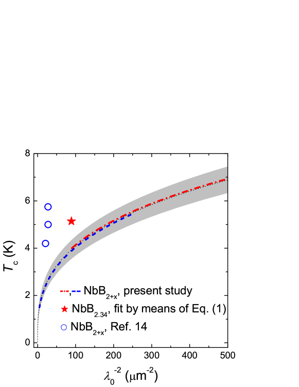
In Fig. 6 we plot $T_{c}$ vs. $\lambda_{0}^{-2}$ dependence obtained from the fit of NbB_2.34 and NbB_2.2 data. The grey area represents the region where $\lambda_{0}^{-2}=[(1.24\pm 0.03)\cdot 10^{-2}\cdot T_{c}]^{3.1\pm 0.1}$. The dotted line corresponds to $\lambda_{0}^{-2}=[1.24\cdot 10^{-2}\cdot T_{c}]^{3.1}$. The dashed blue and the dot-dashed red lines represent the range of the transition temperatures where $T_{c}$ vs. $\lambda_{0}^{-2}$ dependences were reconstructed for NbB_2.2 and NbB_2.34, respectively. For clarity, these lines are shifted by 0.05 K above and below the central $(1.24\cdot 10^{-2}\cdot T_{c})^{3.1}$ line. We also include in this graph data points for NbB_2+x ($x=0.0$, 0.01, and 0.1) from Ref. Takagiwa04, . It is seen that these samples have approximately twice as high transition temperatures as one would expect from the obtained $T_{c}$ vs. $\lambda_{0}^{-2}$ dependence. On the base of our results, we can argue that samples studied in Ref. Takagiwa04, also have distributions of the superconducting volume fractions, similar to what is observed in the present study. Without taking into account this distributions, fit of $\sigma_{sc}(T)$ data can lead to a substantial overestimate of the superconducting transition temperature $T_{c}$. As an example, the star in Fig. 6 represents result of the fit of Eq. (1) to $\sigma_{sc}(T)$ NbB_2.2 data when all measured points are taken equally into account.

Now we are going to comment shortly the observed $T_{c}$ vs. $\lambda_{0}^{-2}$ dependence. Recently it was shown that the famous ”Uemura“ relation, establishing the linear proportionality between $T_{c}$ and $\lambda^{-2}_{0}$,Uemura89 ; Uemura91 does not hold for highly underdoped HTS’s.Zuev05 ; Liang05 ; Sonier07 Indeed, for YBa₂Cu₃O_7-δ Zuev et al. Zuev05 observed $\lambda^{-2}_{0}\propto T_{c}^{2.3(4)}$ and found that this power law is in fairly good agreement with YBa₂Cu₃O_7-δ data in the whole doping range. For the similar compounds Sonier et al. Sonier07 obtained $n=2.6-3.1$. Those values are very close to $3.1(1)$ obtained in the present study for NbB_2+x superconductor. The observation of the power law type of relation between the transition temperature $T_{c}$ and the superfluid density in BCS supercondutor NbB_2+x and their good correspondence to what is observed in HTS’s points to close similarity between these materials. It, probably, comes from the fact that the increase of $T_{c}$ in NbB_2+x, similar to HTS, is determined by increasing the charge carrier concentration.Takagiwa04 ; Escamilla06 Indeed, the x-ray photoelectron spectroscopy experiments of Escamilla and Huerta Escamilla06 show that the increase of boron content leads to a decrease in the contribution of the Nb $4d$ states and increase in the contribution of the B $2p_{\pi}$ states to the density of states at the Fermi level.

Figure 7: (Color online) Dependence of the transition temperature normalized to the maximum transition temperature of the superconducting family ($T_{c}/T_{c}^{max}$) on the normalized inverse squared zero-temperature magnetic penetration depth [$\lambda_{0}^{-2}/(\lambda^{max}_{0})^{-2}]$. Solid line corresponds to $\lambda_{0}^{-2}\propto T_{c}^{3.1}$ as obtained in the present study. Blue diamonds are the Mg_1-xAl_xB₂ data from Ref. Serventi04, . Red stars are the data points for YBa₂Cu₃O_7-δ from Ref. Sonier07, .

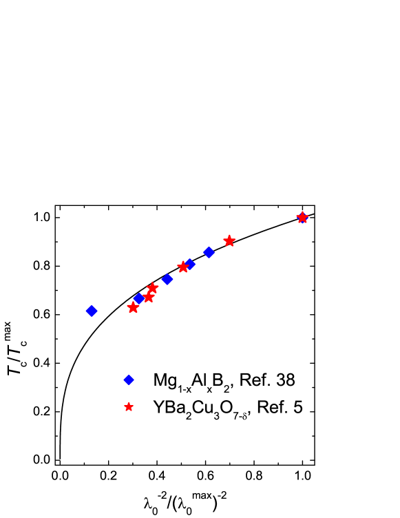
It is important to emphasize that observation of correlation between $T_{c}$ and $\lambda^{-2}_{0}$ in BCS superconductors is not restricted to the particular NbB_2+x system studied here. As an example, in Fig. 7 we plot $T_{c}/T_{c}^{max}$ as a function $\lambda_{0}^{-2}/(\lambda^{max}_{0})^{-2}$ for Al doped MgB₂ from Ref. Serventi04, . Here $T_{c}^{max}$ is the maximum $T_{c}$ of a certain superconducting family and $\lambda^{max}_{0}$ is the corresponding zero temperature penetration depth. We also include on this graph points for YBa₂Cu₃O_7-δ from Ref. Sonier07, . It is seen that all these superconductors represent the very similar relations. The scaling relation for the BCS superconductors, reported here, and their agreement with what was observed in high-temperature cuprate superconductors Zuev05 ; Liang05 ; Sonier07 strongly suggests that there are some features of their electronic properties that are common, despite these materials have quite different dimensionality, Fermi surface topology, symmetry of the superconducting order parameter etc.

V Conclusions

Muon-spin rotation studies were performed on BCS superconductors NbB_2+x ($x=0.2$, 0.34). As a real space microscopic probe, $\mu$SR allows to distinguish between the superconducting and nonsuperconducting parts of the samples and determine the distributions of the superconducting volume fractions with different $T_{c}$’s. By using the model, developed for a granular superconductor of moderate quality, the dependence of the zero-temperature superfluid density $\rho_{s}\propto\lambda^{-2}_{0}$ on the transition temperature $T_{c}$ was reconstructed in a broad range of temperatures ($1.5$ K$\lesssim T_{c}\lesssim 8.0$ K) revealing $\rho_{s}\propto\lambda^{-2}_{0}\propto T_{c}^{3.1(1)}$. This dependence appears to be common at least for some families of BCS superconductors as, e.g., Al doped MgB₂ and high-temperature cuprate superconductors as, e.g. YBa₂Cu₃O_7-δ.

VI Acknowledgments

This work was partly performed at the Swiss Muon Source (S$\mu$S), Paul Scherrer Institute (PSI, Switzerland). The authors are grateful to T. Schneider for stimulating discussions, and A. Amato and D. Herlach for assistance during the $\mu$SR measurements. This work was supported by the Swiss National Science Foundation, by the K. Alex Müller Foundation, and in part by the SCOPES grant No. IB7420-110784 and the EU Project CoMePhS.

References

- (1) Y.J. Uemura , G.M. Luke, B.J. Sternlieb, J.H. Brewer, J.F. Carolan, W.N. Hardy, R. Kadono, J.R. Kempton, R.F. Kiefl, S.R. Kreitzman, P. Mulhern, T.M. Riseman, D.Ll. Williams, B.X. Yang, S. Uchida, H. Takagi, J. Gopalakrishnan, A.W. Sleight, M.A. Subramanian, C.L. Chien, M.Z. Cieplak, Gang Xiao, V.Y. Lee, B.W. Statt, C.E. Stronach, W.J. Kossler, and X.H. Yu, Phys. Rev. Lett. 62, 2317 (1989).
- (2) Y.J. Uemura, L.P. Le, G.M. Luke, B.J. Sternlieb, W.D. Wu, J.H. Brewer, T.M. Riseman, C.L. Seaman, M.B. Maple, M. Ishikawa, D.G. Hinks, J.D. Jorgensen, G. Saito, and H. Yamochi, Phys. Rev. Lett. 66, 2665 (1991).
- (3) Yu. Zuev, M.S. Kim, and T.R. Lemberger, Phys. Rev. Lett. 95, 137002 (2005).
- (4) R. Liang, D.A. Bonn, W.N. Hardy, and D. Broun, Phys. Rev. Lett. 94, 117001 (2005).
- (5) J.E. Sonier, S.A. Sabok-Sayr, F.D. Callaghan, C.V. Kaiser, V. Pacradouni, J.H. Brewer, S.L. Stubbs, W.N. Hardy, D.A. Bonn, R. Liang, and W.A. Atkinson, to appear in Phys. Rev. B, arXiv:0706.2882.
- (6) F.L. Pratt and S.J. Blundell, Phys. Rev. Lett. 94, 097006 (2005).
- (7) K. Kim and P.B. Weichman, Phys. Rev. B 43, 13583 (1991).
- (8) T. Schneider and J.M. Singer, Phase Transition Approach to High Temperature Superconductivity (Imperial College Press, London, 2000).
- (9) T. Schneider, in The Physics of Superconductors (edited by K. H. Bennemann and J. B. Ketterson, Springer, Berlin, 2004).
- (10) T. Schneider, arXiv:cond-mat/0702468.
- (11) H. Kotegawa, K. Ishida, Y. Kitaoka, T. Muranaka, N. Nakagawa, H. Takagiwa, and J. Akimitsu, Physica C 378-381, 25 (2002).
- (12) T. Takasaki, T. Ekino, H. Takagiwa, T. Muranaka, H. Fujii, and J. Akimitsu, Physica C 412-414, 266 (2004).
- (13) T. Ekino, T. Takasaki, H. Takagiwa, J. Akimitsu, and H. Fujii, Physica C 408-410, 828 (2004).
- (14) E. Regalado and R. Escamilla, J. Phys.: Condens. Matter 19, 376209 (2007).
- (15) H. Takagiwa, S. Kuroiwa, M. Yamazawa, J. Akimitsu, K. Ohishi, A. Koda, W. Higemoto, and R. Kadono, J. Phys. Soc. Jpn. 74, 1386 (2005).
- (16) R. Escamilla, O. Lovera, T. Akachi, A. Duran, R. Falconi, F. Morales, and R. Escudero, J. Phys.: Condens. Matter 16, 5979 (2004).
- (17) A. Yamamoto, C. Takao, T. Masui, M. Izumi, and S. Tajima, Physica C 383, 197 (2002).
- (18) M. Tinkham, ”Introduction to Superconductivity“, Krieger Publishing company, Malabar, Florida, 1975.
- (19) R.S. Gonnelli, D. Daghero, G.A. Ummarino, A. Calzolari, M. Tortello, V.A. Stepanov, N.D. Zhigadlo, K. Rogacki, J. Karpinski, F. Bernardini, and S. Massidda, Phys. Rev. Lett. 97, 037001 (2006).
- (20) R. Khasanov, D.G. Eshchenko, J. Karpinski, S.M. Kazakov, N.D. Zhigadlo, R. Brütsch, D. Gavillet, D. Di Castro, A. Shengelaya, F. La Mattina, A. Maisuradze, C. Baines, and H. Keller, Phys. Rev. Lett. 93, 157004 (2004).
- (21) B. Mühlschlegel, Z. Phys. 155, 313 (1959).
- (22) E.H. Brandt, Phys. Rev. B 68, 054506 (2003).
- (23) M. Weber, A. Amato, F.N. Gygax, A. Schenck, H. Maletta, V.N. Duginov, V.G. Grebinnik, A.B. Lazarev, V.G. Olshevsky, V.Yu. Pomjakushin, S.N. Shilov, V.A. Zhukov, B.F. Kirillov, A.V. Pirogov, A.N. Ponomarev, V.G. Storchak, S. Kapusta, and J. Bock, Phys. Rev. B 48, 13022 (1993).
- (24) R. Khasanov, D.G. Eshchenko, D.Di Castro, A. Shengelaya, F.La Mattina, A. Maisuradze, C. Baines, H. Luetkens, J. Karpinski, S.M. Kazakov, and H. Keller, Phys. Rev. B 72, 104504 (2005).
- (25) B. Pümpin, H. Keller, W. Kündig, W. Odermatt, I.M. Savić, J.W. Schneider, H. Simmler, P. Zimmermann, E. Kaldis, S. Rusiecki, Y. Maeno, and C. Rossel, Phys. Rev. B 42, 8019 (1990).
- (26) E.H. Brandt, Phys. Rev. B 37, 2349 (1988).
- (27) E.H. Brandt, Phys. Rev. Lett. 78, 2208 (1997).
- (28) M. Laulajainen, F.D. Callaghan, C.V. Kaiser, and J.E. Sonier, Phys. Rev. B 74, 054511 (2006).
- (29) For clean superconductor the zero temperature value of . For [see Eq. (8)] as well leading to .
- (30) D. Herlach, G. Majer, J. Major, J. Rosenkranz, M. Schmolz, W. Schwarz, A. Seeger, W. Templ, E.H. Brandt, U. Essmann, K. Furderer, and M. Gladisch, Hyperfine Interact. 63, 41 (1990).
- (31) J. Sonier, J. Brewer, and R. Kiefl, Rew. Mod. Phys. 72, 769 (2000).
- (32) R. Khasanov et al., unpublished.
- (33) A. Schenck, Muon Spin Rotation: Principles and Applications in Solid State Physics, (Adam Hilger, Bristol, 1986); S.F.J. Cox, J. Phys. C20, 3187 (1987); J.H. Brewer, “Muon Spin Rotation/Relaxation/Resonance” in Encyclopedia of Applied Physics Vol. 11, p. 23 (VCH, New York, 1995).
- (34) B.D. Rainford and G.J. Daniell, Hyperfine Interact. 87, 1129 (1994).
- (35) P. Zimmermann, H. Keller, S. L. Lee, I. M. Savic, M. Warden, D. Zech, R. Cubitt, E. M. Forgan, E. Kaldis, J. Karpinski, and C. Krüger, Phys. Rev. B 52, 541 (1995).
- (36) A. Koda, W. Higemoto, K. Ohishi, S.R. Saha, R. Kadono, S. Yonezawa, Y. Muraoka, and Z. Hiroi, J. Phys. Soc. Jpn. 74, 1678 (2005).
- (37) R. Escamilla and L. Huerta, Supercond. Sci. Technol. 19, 623 (2006).
- (38) S. Serventi, G. Allodi, R.De Renzi, G. Guidi, L. Romano, P. Manfrinetti, A. Palenzona, Ch. Niedermayer, A. Amato, and Ch. Baines, Phys. Rev. Lett. 93, 217003 (2004).