Mixed finite element methods for the fully nonlinear Monge-Ampère equation based on the vanishing moment method

Abstract

This paper studies mixed finite element approximations of the viscosity solution to the Dirichlet problem for the fully nonlinear Monge-Ampère equation $\det(D^{2}u^{0})=f\,(>0)$ based on the vanishing moment method which was proposed recently by the authors in [19]. In this approach, the second order fully nonlinear Monge-Ampère equation is approximated by the fourth order quasilinear equation $-\varepsilon\Delta^{2}u^{\varepsilon}+\det{D^{2}u^{\varepsilon}}=f$. It was proved in [17] that the solution $u^{\varepsilon}$ converges to the unique convex viscosity solution $u^{0}$ of the Dirichlet problem for the Monge-Ampère equation. This result then opens a door for constructing convergent finite element methods for the fully nonlinear second order equations, a task which has been impracticable before. The goal of this paper is threefold. First, we develop a family of Hermann-Miyoshi type mixed finite element methods for approximating the solution $u^{\varepsilon}$ of the regularized fourth order problem, which computes simultaneously $u^{\varepsilon}$ and the moment tensor $\sigma^{\varepsilon}:=D^{2}u^{\varepsilon}$. Second, we derive error estimates, which track explicitly the dependence of the error constants on the parameter ${\varepsilon}$, for the errors $u^{\varepsilon}-u^{\varepsilon}_{h}$ and $\sigma^{\varepsilon}-\sigma_{h}^{\varepsilon}$. 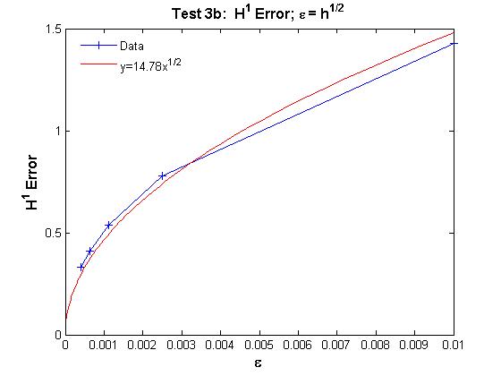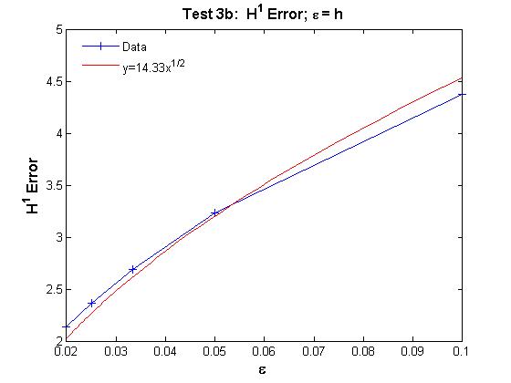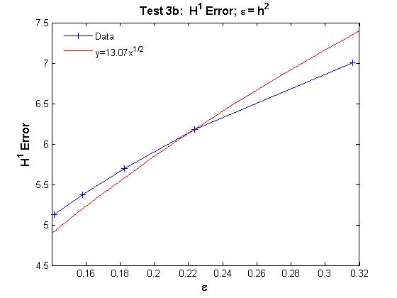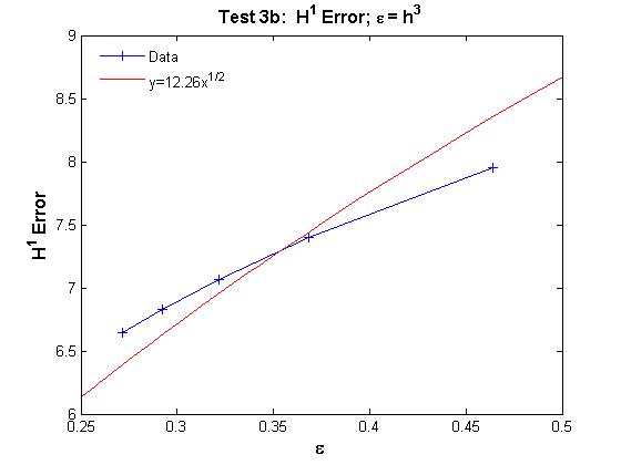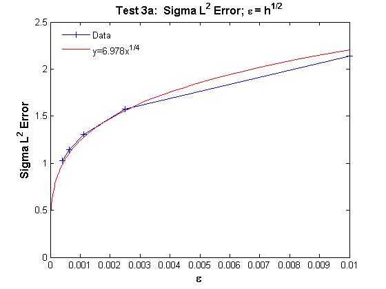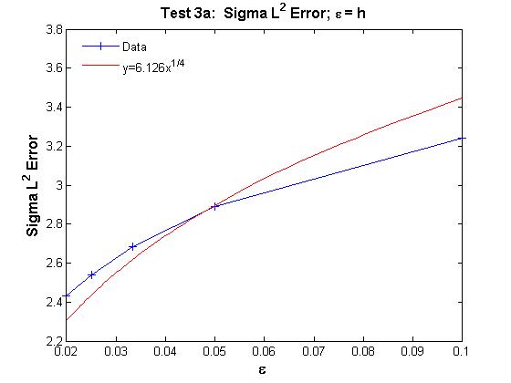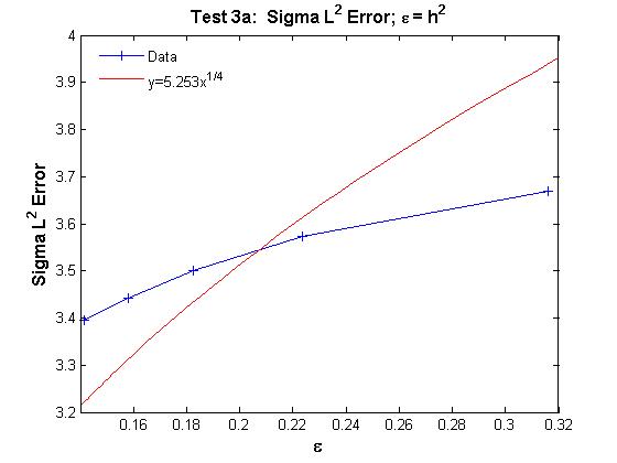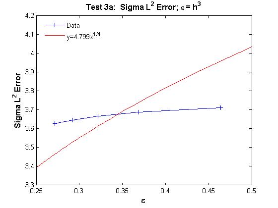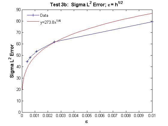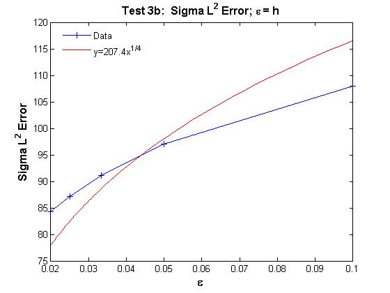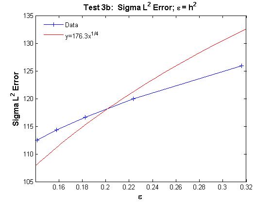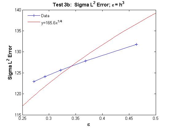Finally, we present a detailed numerical study on the rates of convergence in terms of powers of ${\varepsilon}$ for the error $u^{0}-u_{h}^{\varepsilon}$ and $\sigma^{\varepsilon}-\sigma_{h}^{\varepsilon}$, and numerically examine what is the “best” mesh size $h$ in relation to ${\varepsilon}$ in order to achieve these rates. Due to the strong nonlinearity of the underlying equation, the standard perturbation argument for error analysis of finite element approximations of nonlinear problems does not work for the problem. To overcome the difficulty, we employ a fixed point technique which strongly relies on the stability of the linearized problem and its mixed finite element approximations.

1 Introduction

This paper is the second in a sequence (cf. [20]) which concerns with finite element approximations of viscosity solutions of the following Dirichlet problem for the fully nonlinear Monge-Ampère equation (cf. [23]):

(1) $$\det(D^{2}u^{0}) =f \qquad\text{in }\Omega\subset\mathbf{R}^{n},$$

(2) $$u^{0} =g \qquad\text{on }\partial\Omega,$$

where $\Omega$ is a convex domain with smooth boundary ${\partial}{\Omega}$. $D^{2}u^{0}(x)$ and $\det(D^{2}u^{0}(x))$ denote the Hessian of $u^{0}$ at $x\in{\Omega}$ and the determinant of $D^{2}u^{0}(x)$.

The Monge-Ampère equation is a prototype of fully nonlinear second order PDEs which have a general form

(3) $$F(D^{2}u^{0},Du^{0},u^{0},x)=0$$

with $F(D^{2}u^{0},Du^{0},u^{0},x)=\det(D^{2}u^{0})-f$. The Monge-Ampère equation arises naturally from differential geometry and from applications such as mass transportation, meteorology, and geostrophic fluid dynamics [4, 8]. It is well-known that for non-strictly convex domain ${\Omega}$ the above problem does not have classical solutions in general even $f$, $g$ and ${\partial}{\Omega}$ are smooth (see [22]). Classical result of A. D. Aleksandrov states that the Dirichlet problem with $f>0$ has a unique generalized solution in the class of convex functions (cf. [1, 9]). Major progress on analysis of problem (1)-(2) has been made later after the introduction and establishment of the viscosity solution theory (cf. [7, 12, 23]). We recall that the notion of viscosity solutions was first introduced by Crandall and Lions [11] in 1983 for the first order fully nonlinear Hamilton-Jacobi equations. It was quickly extended to second order fully nonlinear PDEs, with dramatic consequences in the wake of a breakthrough of Jensen’s maximum principle [25] and the Ishii’s discovery [24] that the classical Perron’s method could be used to infer existence of viscosity solutions. To continue our discussion, we need to recall the definition of viscosity solutions for the Dirichlet Monge-Ampère problem (1)-(2) (cf. [23]).

Definition 1.

a convex function $u^{0}\in C^{0}(\overline{{\Omega}})$ satisfying $u^{0}=g$ on ${\partial}{\Omega}$ is called a viscosity subsolution (resp. viscosity supersolution) of (1) if for any $\varphi\in C^{2}$ there holds $\det(D^{2}\varphi(x_{0}))\leq f(x_{0})$ (resp. $\det(D^{2}\varphi(x_{0}))\geq f(x_{0})$) provided that $u^{0}-\varphi$ has a local maximum (resp. a local minimum) at $x_{0}\in{\Omega}$. $u^{0}\in C^{0}(\overline{{\Omega}})$ is called a viscosity solution if it is both a viscosity subsolution and a viscosity supersolution.

It is clear that the notion of viscosity solutions is not variational. It is based on a “differentiation by parts” approach, instead of the more familiar integration by parts approach. As a result, it is not possible to directly approximate viscosity solutions using Galerkin type numerical methods such as finite element, spectral and discontinuous Galerkin methods, which all are based on variational formulations of PDEs. The situation also presents a big challenge and paradox for the numerical PDE community, since, on one hand, the “differentiation by parts” approach has worked remarkably well for establishing the viscosity solution theory for fully nonlinear second order PDEs in the past two decades; on the other hand, it is extremely difficult (if all possible) to mimic this approach at the discrete level. It should be noted that unlike in the case of fully nonlinear first order PDEs, the terminology “viscosity solution” loses its original meaning in the case of fully nonlinear second order PDEs.

Motivated by this difficulty and by the goal of developing convergent Galerkin type numerical methods for fully nonlinear second order PDEs, very recently we proposed in [17] a new notion of weak solutions, called moment solutions, which is defined using a constructive method, called the vanishing moment method. The main idea of the vanishing moment method is to approximate a fully nonlinear second order PDE by a quasilinear higher order PDE. The notion of moment solutions and the vanishing moment method are natural generalizations of the original definition of viscosity solutions and the vanishing viscosity method introduced for the Hamilton-Jacobi equations in [11]. We now briefly recall the definitions of moment solutions and the vanishing moment method, and refer the reader to [17, 19] for a detailed exposition.

The first step of the vanishing moment method is to approximate the fully nonlinear equation (3) by the following quasilinear fourth order PDE:

(4) $$-{\varepsilon}\Delta^{2}u^{\varepsilon}+F(D^{2}u^{\varepsilon},Du^{\varepsilon},u^{\varepsilon},x)=0\hskip 28.45274pt\ \ (\varepsilon>0),$$

which holds in domain ${\Omega}$. Suppose the Dirichlet boundary condition $u^{0}=g$ is prescribed on the boundary ${\partial}{\Omega}$, then it is natural to impose the same boundary condition on $u^{\varepsilon}$, that is,

(5) $$u^{\varepsilon}=g\qquad\text{on }{\partial}{\Omega}.$$

However, boundary condition (5) alone is not sufficient to ensure uniqueness for fourth order PDEs. An additional boundary condition must be imposed. In [17] the authors proposed to use one of the following (extra) boundary conditions:

(6) $$\Delta u^{\varepsilon}={\varepsilon},\quad\text{or}\quad D^{2}u^{\varepsilon}\nu\cdot\nu=\varepsilon\hskip 28.45274pt\text{on}\ \partial\Omega,$$

where $\nu$ stands for the unit outward normal to ${\partial}{\Omega}$. Although both boundary conditions work well numerically, the first boundary condition $\Delta u^{\varepsilon}={\varepsilon}$ is more convenient for standard finite element methods, spectral and discontinuous Galerkin methods (cf. [20]), while the second boundary condition $D^{2}u^{\varepsilon}\nu\cdot\nu=\varepsilon$ fits better for mixed finite element methods, and hence, it will be used in this paper.

In summary, the vanishing moment method involves approximating second order boundary value problem (2)–(3) by fourth order boundary value problem (4)–(5), (6). In the case of the Monge-Ampère equation, this means that we approximate boundary value problem (1)–(2) by the following problem:

(7) $$-{\varepsilon}\Delta^{2}u^{\varepsilon}+\text{det}(D^{2}u^{\varepsilon}) =f\hskip 28.45274pt \text{in}\ \Omega,$$

(8) $$u^{\varepsilon} =g\hskip 28.45274pt \text{on}\ \partial\Omega,$$

(9) $$D^{2}u^{\varepsilon}\nu\cdot\nu =\varepsilon\hskip 28.45274pt \text{on}\ \partial\Omega.$$

It was proved in [19] that if $f>0$ in ${\Omega}$ then problem (7)–(9) has a unique solution $u^{\varepsilon}$ which is a strictly convex function over ${\Omega}$. Moreover, $u^{\varepsilon}$ uniformly converges as ${\varepsilon}\to 0$ to the unique viscosity solution of (1)–(2). As a result, this shows that (1)–(2) possesses a unique moment solution that coincides with the unique viscosity solution. Furthermore, it was proved that there hold the following a priori bounds which will be used frequently later in this paper:

(10) $$\|u^{\varepsilon}\|_{H^{j}}=O\bigl{(}\varepsilon^{-\frac{j-1}{2}}\bigr{)}, \qquad\|u^{\varepsilon}\|_{W^{2,\infty}}=O\bigl{(}\varepsilon^{-1}\bigr{)},$$

(11) $$\|D^{2}u^{\varepsilon}\|_{L^{2}}=O\bigl{(}\varepsilon^{-\frac{1}{2}}\bigr{)}, \qquad\|\text{cof}(D^{2}u^{\varepsilon})\|_{L^{\infty}}=O\bigl{(}\varepsilon^{-1}\bigr{)}$$

for $j=2,3$. Where $\text{cof}(D^{2}u^{\varepsilon})$ denotes the cofactor matrix of the Hessian, $D^{2}u^{\varepsilon}$.

With the help of the vanishing moment methodology, the original difficult task of computing the unique convex viscosity solution of the fully nonlinear Monge-Ampère problem (1)–(2), which has multiple solutions (i.e. there are non-convex solutions), is now reduced to a feasible task of computing the unique regular solution of the quasilinear fourth order problem (7)–(9). This then opens a door to let one use and/or adapt the wealthy amount of existing numerical methods, in particular, finite element Galerkin methods to solve the original problem (1)–(2) via the problem (7)–(9).

The goal of this paper is to construct and analyze a class of Hermann-Miyoshi type mixed finite element methods for approximating the solution of (7)–(9). In particular, we are interested in deriving error bounds that exhibit explicit dependence on ${\varepsilon}$. We note that finite element approximations of fourth order PDEs, in particular, the biharmonic equation, were carried out extensively in 1970’s in the two-dimensional case (see [10] and the references therein), and have attracted renewed interests lately for generalizing the well-know $2$-D finite elements to the $3$-D case (cf. [35, 36, 34]) and for developing discontinuous Galerkin methods in all dimensions (cf. [18, 27]). Clearly, all these methods can be readily adapted to discretize problem (7)–(9) although their convergence analysis do not come easy due to the strong nonlinearity of the PDE (7). We refer the reader to [20, 28] for further discussions in this direction.

A few attempts and results on numerical approximations of the Monge-Ampère as well as related equations have recently been reported in the literature. Oliker and Prussner [30] constructed a finite difference scheme for computing Aleksandrov measure induced by $D^{2}u$ in $2$-D and obtained the solution $u$ of problem (7)–(9) as a by-product. Baginski and Whitaker [2] proposed a finite difference scheme for Gauss curvature equation (cf. [19] and the references therein) in $2$-D by mimicking the unique continuation method (used to prove existence of the PDE) at the discrete level. In a series of papers (cf. [13] and the references therein) Dean and Glowinski proposed an augmented Lagrange multiplier method and a least squares method for problem (7)–(9) and the Pucci’s equation (cf. [7, 22]) in $2$-D by treating the Monge-Ampère equation and Pucci’s equation as a constraint and using a variational criterion to select a particular solution. Very recently, Oberman [29] constructed some wide stencil finite difference scheme which fulfill the convergence criterion established by Barles and Souganidis in [3] for finite difference approximations of fully nonlinear second order PDEs. Consequently, the convergence of the proposed wide stencil finite difference scheme immediately follows from the general convergence framework of [3]. Numerical experiments results were reported in [30, 29, 2, 13], however, convergence analysis was not addressed except in [29].

The remainder of this paper is organized as follows. In Section 2, we first derive the Hermann-Miyoshi mixed weak formulation for problem (7)-(9) and then present our mixed finite element methods based on this weak formulation. Section 3 is devoted to studying the linearization of problem (7)-(9) and its mixed finite element approximations. The results of this section, which are of independent interests in themselves, will play a crucial role in our error analysis for the mixed finite element introduced in Section 2. In Section 4, we establish error estimates in the energy norm for the proposed mixed finite element methods. Our main ideas are to use a fixed point technique and to make strong use of the stability property of the linearized problem and its finite element approximations, which all are established in Section 3. In addition, we derive the optimal order error estimate in the $H^{1}$-norm for $u^{\varepsilon}-u^{\varepsilon}_{h}$ using a duality argument. Finally, in Section 5, we first run some numerical tests to validate our theoretical error estimate results, we then present a detailed computational study for determining the “best” choice of mesh size $h$ in terms of $\varepsilon$ in order to achieve the optimal rates of convergence, and for estimating the rates of convergence for both $u^{0}-u^{\varepsilon}_{h}$ and $u^{0}-u^{\varepsilon}$ in terms of powers of $\varepsilon$.

We conclude this section by remarking that standard space notations are adopted in this paper, we refer to [5, 22, 10] for their exact definitions. In addition, ${\Omega}$ denotes a bounded domain in $\mathbf{R}^{n}$ for $n=2,3$. $(\cdot,\cdot)$ and $\langle\cdot,\cdot\rangle$ denote the $L^{2}$-inner products on ${\Omega}$ and on ${\partial}{\Omega}$, respectively. For a Banach space $B$, its dual space is denoted by $B^{*}$. $C$ is used to denote a generic ${\varepsilon}$-independent positive constant.

2 Formulation of mixed finite element methods

There are several popular mixed formulations for fourth order problems (cf. [6, 10, 16]). However, since the Hessian matrix, $D^{2}u^{\varepsilon}$ appears in (7) in a nonlinear fashion, we cannot use $\Delta u^{\varepsilon}$ alone as our additional variables, but rather we are forced to use $\sigma^{\varepsilon}:=D^{2}u^{\varepsilon}$ as a new variable. Because of this, we rule out the family of Ciarlet-Raviart mixed finite elements (cf. [10]). On the other hand, this observation suggests to try Hermann-Miyoshi or Hermann-Johnson mixed elements (cf. [6, 16]), which both seek $\sigma^{\varepsilon}$ as an additional unknown. In this paper, we shall only focus on developing Hermann-Miyoshi type mixed methods.

We begin with a few more space notation:

$$V:=H^{1}(\Omega),\hskip 28.45274pt W:=\{\mu\in[H^{1}(\Omega)]^{n\times n};\ \mu_{ij}=\mu_{ji}\},$$

$$V_{0}:=H^{1}_{0}({\Omega}),\hskip 28.45274pt V_{g}:=\{v\in V;\ v|_{\partial\Omega}=g\},$$

$$W_{\varepsilon}:=\{\mu\in W;\ \mu n\cdot n|_{\partial\Omega}=\varepsilon\},\hskip 28.45274pt W_{0}:=\{\mu\in W;\ \mu n\cdot n|_{\partial\Omega}=0\}.$$

To define the Hermann-Miyoshi mixed formulation for problem (7)-(9), we rewrite the PDE into the following system of second order equations:

(12) $$\sigma^{\varepsilon}-D^{2}u^{\varepsilon} = 0,$$

(13) $$-\varepsilon\Delta\text{tr}(\sigma^{\varepsilon})+\text{det}(\sigma^{\varepsilon}) = f.$$

Testing (13) with $v\in V_{0}$ yields

(14) $$\varepsilon\int_{\Omega}\text{div}(\sigma^{\varepsilon})\cdot Dv\,dx+\int_{\Omega}\text{det}(\sigma^{\varepsilon})v\,dx=\int_{\Omega}fv\,dx.$$

Multiplying (12) by $\mu\in W_{0}$ and integrating over $\Omega$ we get

(15) $$\int_{\Omega}\sigma^{\varepsilon}:\mu\,dx+\int_{\Omega}Du^{\varepsilon}\cdot\text{div}(\mu)\,dx=\sum_{k=1}^{n-1}\int_{\partial\Omega}\mu n\cdot\tau_{k}\frac{\partial g}{\partial\tau_{k}}\ ds,$$

where $\sigma^{\varepsilon}:\mu$ denotes the matrix inner product and $\{\tau_{1}(x),\tau_{2}(x)\cdots,\tau_{n-1}(x)\}$ denotes the standard basis for the tangent space to ${\partial}{\Omega}$ at $x$.

From (14) and (15) we define the variational formulation for (12)-(13) as follows: Find $(u^{\varepsilon},\sigma^{\varepsilon})\in V_{g}\times W_{\varepsilon}$ such that

(16) $$(\sigma^{\varepsilon},\mu)+\bigl{(}\text{div}(\mu),Du^{\varepsilon}\bigr{)} =\langle\tilde{g},\mu\rangle\hskip 28.45274pt\forall\mu\in W_{0},$$

(17) $$\bigl{(}\text{div}(\sigma^{\varepsilon}),v\bigr{)}+\frac{1}{\varepsilon}\bigl{(}\text{det}\sigma^{\varepsilon},v\bigr{)} =(f^{\varepsilon},v)\hskip 28.45274pt\forall v\in V_{0},$$

where

$$\langle\tilde{g},\mu\rangle=\sum_{i=1}^{n-1}\Bigl{\langle}\frac{\partial g}{\partial\tau_{i}},\mu n\cdot\tau_{i}\Bigr{\rangle}\quad\text{and}\quad f^{\varepsilon}=\frac{1}{\varepsilon}f.$$

Remark 2.1.

We note that $\text{\rm det}(\sigma^{\varepsilon})=\frac{1}{n}\Phi^{\varepsilon}D^{2}u^{\varepsilon}=\frac{1}{n}\sum_{i=1}^{n}\Phi^{\varepsilon}_{ij}u^{\varepsilon}_{x_{i}x_{j}}$ for $j=1,2,...,n$, where $\Phi^{\varepsilon}=\text{\rm cof}(\sigma^{\varepsilon})$, the cofactor matrix of $\sigma^{\varepsilon}:=D^{2}u^{\varepsilon}$. Thus, using the divergence free property of the cofactor matrix $\Phi^{\varepsilon}$ (cf. Lemma 3.1) we can define the following alternative variational formulation for (12)-(13):

$$(\sigma^{\varepsilon},\mu)+\bigl{(}{\mbox{\rm div}}(\mu),Du^{\varepsilon}\bigr{)} =\langle\tilde{g},\mu\rangle\hskip 28.45274pt\forall\mu\in W_{0},$$

$$({\mbox{\rm div}}(\sigma^{\varepsilon}),Dv)-\frac{1}{\varepsilon n}\bigl{(}\Phi^{\varepsilon}Du^{\varepsilon},Dv\bigr{)} =(f^{\varepsilon},v)\hskip 28.45274pt\forall v\in V_{0}.$$

However, we shall not use the above weak formulation in this paper although it is interesting to compare mixed finite element methods based on the above two different but equivalent weak formulations.

To discretize (16)–(17), let $T_{h}$ be a quasiuniform triangular or rectangular partition of ${\Omega}$ if $n=2$ and be a quasiuniform tetrahedral or $3$-D rectangular mesh if $n=3$. Let $V^{h}\subset H^{1}(\Omega)$ be the Lagrange finite element space consisting of continuous piecewise polynomials of degree $k(\geq 2)$ associated with the mesh $T_{h}$. Let

$$V_{g}^{h}:=V^{h}\cap V_{g},\hskip 28.45274pt V_{0}^{h}:=V^{h}\cap V_{0},$$

$$W_{\varepsilon}^{h}:=[V^{h}]^{n\times n}\cap W_{\varepsilon},\hskip 28.45274pt W^{h}_{0}:=[V^{h}]^{n\times n}\cap W_{0}.$$

In the $2$-D case, the above choices of $V_{0}^{h}$ and $W_{0}^{h}$ are known as the Hermann-Miyoshi mixed finite element for the biharmonic equation (cf. [6, 16]). They form a stable pair which satisfies the inf-sup condition. We like to note that it is easy to check that the Hermann-Miyoshi mixed finite element also satisfies the inf-sup condition in $3$-D. See Section 3.2 for the details.

Based on the weak formulation (16)-(17) and using the above finite element spaces we now define our Hermann-Miyoshi type mixed finite element method for (7)–(9) as follows: Find $(u_{h}^{\varepsilon},\sigma_{h}^{\varepsilon})\in V^{h}_{g}\times W^{h}_{\varepsilon}$ such that

(18) $$(\sigma^{\varepsilon}_{h},\mu_{h})+\bigl{(}{\mbox{\rm div}}(\mu_{h}),Du^{\varepsilon}_{h}\bigr{)} =\langle\tilde{g},\mu_{h}\rangle\hskip 28.45274pt\forall\mu_{h}\in W^{h}_{0},$$

(19) $$\bigl{(}{\mbox{\rm div}}(\sigma^{\varepsilon}_{h}),Dv_{h}\bigr{)}+\frac{1}{\varepsilon}\bigl{(}\det(\sigma^{\varepsilon}_{h}),v_{h}\bigr{)} =(f^{\varepsilon},v_{h})\hskip 28.45274pt\forall v_{h}\in V^{h}_{0}.$$

Let $(\sigma^{\varepsilon},u^{\varepsilon})$ be the solution to (16)-(17) and $(\sigma^{\varepsilon}_{h},u^{\varepsilon}_{h})$ solves (18)-(19). As mentioned in Section 1, the primary goal of this paper is derive error estimates for $u^{\varepsilon}-u^{\varepsilon}_{h}$ and $\sigma^{\varepsilon}-\sigma^{\varepsilon}_{h}$. To the end, we first need to prove existence and uniqueness of $(\sigma^{\varepsilon}_{h},u^{\varepsilon}_{h})$. It turns out both tasks are not easy to accomplish due to the strong nonlinearity in (19). Unlike in the continuous PDE case where $u^{\varepsilon}$ is proved to be convex for all ${\varepsilon}$ (cf. [19]), it is far from clear if $u^{\varepsilon}_{h}$ preserves the convexity even for small ${\varepsilon}$ and $h$. Without a guarantee of convexity for $u^{\varepsilon}_{h}$, we could not establish any stability result for $u^{\varepsilon}_{h}$. This in turn makes proving existence and uniqueness a difficult and delicate task. In addition, again due to the strong nonlinearity, the standard perturbation technique for deriving error estimate for numerical approximations of mildly nonlinear problems does not work here. To overcome the difficulty, our idea is to adopt a combined fixed point and linearization technique which was used by the authors in [21], where a nonlinear singular second order problem known as the inverse mean curvature flow was studied. We note that this combined fixed point and linearization technique kills three birds by one stone, that is, it simultaneously proves existence and uniqueness for $u^{\varepsilon}_{h}$ and also yields the desired error estimates. In the next two sections, we shall give the detailed account about the technique and realize it for problem (18)-(19).

3 Linearized problem and its finite element approximations

To build the necessary technical tools, in this section we shall derive and present a detailed study of the linearization of (16)-(17) and its mixed finite element approximations, First, we recall the following divergence-free row property for the cofactor matrices, which will be frequently used in later sections. We refer to [15, p.440] for a short proof of the lemma.

Lemma 3.1.

Given a vector-valued function $\mathbf{v}=(v_{1},v_{2},\cdots,v_{n}):{\Omega}\rightarrow\mathbb{R}^{n}$. Assume $\mathbf{v}\in[C^{2}({\Omega})]^{n}$. Then the cofactor matrix $\text{\rm cof}(D\mathbf{v})$ of the gradient matrix $D\mathbf{v}$ of $\mathbf{v}$ satisfies the following row divergence-free property:

(20) $${\mbox{\rm div}}(\text{\rm cof}(D\mathbf{v}))_{i}=\sum_{j=1}^{n}{\partial}_{x_{j}}(\text{\rm cof}(D\mathbf{v}))_{ij}=0\qquad\text{for }i=1,2,\cdots,n,$$

where $(\text{\rm cof}(D\mathbf{v}))_{i}$ and $(\text{\rm cof}(D\mathbf{v}))_{ij}$ denote respectively the $i$th row and the $(i,j)$-entry of $\text{\rm cof}(D\mathbf{v})$.

3.1 Derivation of linearized problem

We note that for a given function $w$ there holds

$$\det(D^{2}u^{\varepsilon}+tw)=\det(D^{2}u^{\varepsilon})+t\text{tr}(\Phi^{\varepsilon}D^{2}w)+\cdots+t^{n}\text{det}(D^{2}w).$$

Thus, setting $t=0$ after differentiating with respect to $t$ we find the linearization of $M^{\varepsilon}(u^{\varepsilon}):=-{\varepsilon}{\Delta}^{2}u^{\varepsilon}+\det(D^{2}u^{\varepsilon})$ at the solution $u^{\varepsilon}$ to be

$$L_{u^{\varepsilon}}(w):=-\varepsilon\Delta^{2}w+\text{tr}(\Phi^{\varepsilon}D^{2}w)=-\varepsilon\Delta^{2}w+\Phi^{\varepsilon}:D^{2}w=-\varepsilon\Delta^{2}w+{\mbox{\rm div}}(\Phi^{\varepsilon}Dw),$$

where we have used (20) with $\mathbf{v}=Du^{\varepsilon}$.

We now consider the following linear problem:

(21) $$L_{u^{\varepsilon}}(w) =q\hskip 28.45274pt\text{in}\ \Omega,$$

(22) $$w =0\hskip 28.45274pt\text{on}\ \partial\Omega,$$

(23) $$D^{2}w\nu\cdot\nu =0\hskip 28.45274pt\text{on}\ \partial\Omega.$$

To introduce a mixed formulation for (21)-(23), we rewrite the PDE as

(24) $$\chi-D^{2}w =0,$$

(25) $$-\varepsilon\Delta\text{tr}(\chi)+{\mbox{\rm div}}(\Phi^{\varepsilon}Dw) =q.$$

Its variational formulation is then defined as: Given $q\in V^{*}_{0}$, find $(\chi,w)\in W_{0}\times V_{0}$ such that

(26) $$(\chi,\mu)+({\mbox{\rm div}}(\mu),Dw) =0 \hskip 28.45274pt\forall\mu\in W_{0},$$

(27) $$({\mbox{\rm div}}(\chi),Dv)-\frac{1}{\varepsilon}(\Phi^{\varepsilon}Dw,Dv) =\frac{1}{\varepsilon}\langle q,v\rangle \hskip 28.45274pt\forall v\in V_{0}.$$

It is not hard to show that if $(\chi,w)$ solves (26)-(27) then $w\in H^{2}(\Omega)\cap H^{1}_{0}({\Omega})$ should be a weak solution to problem (21)-(23). On the other hand, by the elliptic theory for linear PDEs (cf. [26]), we know that if $q\in V^{*}_{0}$, then the solution to problem (21)-(23) satisfies $w\in H^{3}(\Omega)$, so that $\chi=D^{2}w\in H^{1}(\Omega)$. It is easy to verify that $(w,\chi)$ is a solution to (26)-(27).

3.2 Mixed finite element approximations of the linearized problem

Our finite element method for (26)-(27) is defined by seeking $(\chi_{h},w_{h})\in W^{h}_{0}\times V^{h}_{0}$ such that

(28) $$(\chi_{h},\mu_{h})+(\text{div}(\mu_{h}),Dw_{h}) =0 \hskip 28.45274pt\forall\mu_{h}\in W^{h}_{0},$$

(29) $$(\text{div}(\chi_{h}),Dv_{h})-\frac{1}{\varepsilon}(\Phi^{\varepsilon}Dw_{h},Dv_{h}) =\langle q,v_{h}\rangle \hskip 28.45274pt\forall v_{h}\in V_{0}^{h}.$$

The objectives of this subsection are to first prove existence and uniqueness for problem (28)-(29) and then derive error estimates in various norms. First, we prove the following inf-sup condition for the mixed finite element pair $(W^{h}_{0},V^{h}_{0})$.

Lemma 3.2.

For every $v_{h}\in V^{h}_{0}$, there exists a constant $\beta_{0}>0$, independent of $h$, such that

(30) $$\sup_{\ \mu_{h}\in W^{h}_{0}}\ \frac{\bigl{(}{\mbox{\rm div}}(\mu_{h}),Dv_{h}\bigr{)}}{\|\mu_{h}\|_{H^{1}}}\geq\beta_{0}\|v_{h}\|_{H^{1}}.$$

Proof.

Given $v_{h}\in V^{h}_{0}$, set $\mu_{h}=I_{n\times n}v_{h}$. Then $\bigl{(}{\mbox{\rm div}}(\mu_{h}),Dv_{h}\bigr{)}=\|Dv_{h}\|_{L^{2}}^{2}\geq\beta_{0}\|v_{h}\|_{H^{1}}^{2}=\beta_{0}\|v_{h}\|_{H^{1}}\|\mu_{h}\|_{H^{1}}$. Here we have used Poincare inequality. ∎

Remark 3.1.

By [16, Proposition 1], (30) implies that there exists a linear operator $\Pi_{h}:\ W\to W^{h}$ such that

(31) $$\bigl{(}{\mbox{\rm div}}(\mu-\Pi_{h}\mu),Dv_{h}\bigr{)}=0\hskip 28.45274pt\forall v_{h}\in V^{h}_{0},$$

and for $\mu\in W\cap[H^{r}(\Omega)]^{n\times n},\ r\geq 1$, there holds

(32) $$\|\mu-\Pi_{h}\mu\|_{H^{j}}\leq Ch^{l-j}\|\mu\|_{H^{l}}\ \ \ j=0,1,\quad 1\leq l\leq\min\{k+1,r\}.$$

We note that the above results were proved in the $2$-D case in [16], However, they also hold in the $3$-D case as (30) holds in $3$-D.

Theorem 3.1.

For any $q\in V^{*}_{0}$, there exists a unique solution $(\chi_{h},w_{h})\in W_{0}^{h}\times V_{0}^{h}$ to problem (28)-(29).

Proof.

Since we are in the finite dimensional case and the problem is linear, it suffices to show uniqueness. Thus, suppose $(\chi_{h},w_{h})\in W_{0}^{h}\times V_{0}^{h}$ solves

$$(\chi_{h},\mu_{h})+(\text{div}(\mu_{h}),Dw_{h}) =0\hskip 28.45274pt\forall\mu_{h}\in W_{0}^{h},$$

$$(\text{div}(\chi_{h}),Dv_{h})-\frac{1}{\varepsilon}(\Phi^{\varepsilon}Dw_{h},Dv_{h}) =0\hskip 28.45274pt\forall v_{h}\in V_{0}^{h}.$$

Let $\mu_{h}=\chi_{h}$, $v_{h}=w_{h}$ and subtract two equations to obtain

$$(\chi_{h},\chi_{h})+\frac{1}{\varepsilon}(\Phi^{\varepsilon}Dw_{h},Dw_{h})=0.$$

Since $u^{\varepsilon}$ is strictly convex, then $\Phi^{\varepsilon}$ is positive definite. Thus, there exists $\theta>0$ such that

$$\|\chi_{h}\|_{L^{2}}^{2}+\frac{\theta}{\varepsilon}\|Dw_{h}\|_{L^{2}}^{2}\leq 0.$$

Hence, $\chi_{h}=0,\ w_{h}=0$, and the desired result follows. ∎

Theorem 3.2.

Let $(\chi,w)\in[H^{r}(\Omega)]^{n\times n}\cap W_{0}\times H^{r}(\Omega)\cap V_{0}$ be the solution to (26)-(27) and $(\chi_{h},w_{h})\in W^{h}_{0}\times V^{h}_{0}$ solves (28)–(29). Then there hold

(33) $$\|\chi-\chi_{h}\|_{L^{2}} \leq C\varepsilon^{-\frac{3}{2}}h^{l-2}\bigl{[}\|\chi\|_{H^{l}}+\|w\|_{H^{l}}\bigr{]}$$

(34) $$\|\chi-\chi_{h}\|_{H^{1}} \leq C\varepsilon^{-\frac{3}{2}}h^{l-3}\bigl{[}\|\chi\|_{H^{l}}+\|w\|_{H^{l}}\bigr{]}$$

(35) $$\|w-w_{h}\|_{H^{1}} \leq C\varepsilon^{-3}h^{l-1}\bigl{[}\|\chi\|_{H^{l}}+\|w\|_{H^{l}}\bigr{]},$$

Moreover, for $$k\geq 3$$ there also holds

(36) $$\|w-w_{h}\|_{L^{2}} \leq C\varepsilon^{-5}h^{l}\bigl{[}\|\chi\|_{H^{l}}+\|w\|_{H^{l}}\bigr{]}.$$

Proof.

Let $I_{h}w$ denote the standard finite element interplant of $w$ in $V^{h}_{0}$. Then

(37) $$(\Pi_{h}\chi-\chi_{h},\mu_{h})+(\text{div}(\mu_{h}),D(I_{h}w-w_{h}))$$

$$\hskip 72.26999pt=(\Pi_{h}\chi-\chi,\mu_{h})+({\mbox{\rm div}}(\mu_{h}),D(I_{h}w-w)),$$

(38) $$({\mbox{\rm div}}(\Pi_{h}\chi-\chi_{h}),Dv_{h})-\frac{1}{\varepsilon}\bigl{(}\Phi^{\varepsilon}D(I_{h}w-w_{h}),Dv_{h})$$

$$\hskip 72.26999pt=-\frac{1}{\varepsilon}\bigl{(}\Phi^{\varepsilon}D(I_{h}w-w),Dv_{h}).$$

Let $\mu_{h}=\Pi_{h}-\chi_{h}$ and $v_{h}=I_{h}w-w_{h}$ and subtract (38) from (37) to get

$$(\Pi_{h}\chi-\chi_{h},\Pi_{h}\chi-\chi_{h})+\frac{1}{\varepsilon}\bigl{(}\Phi^{\varepsilon}D(I_{h}w-w_{h}),D(I_{h}w-w_{h})\bigr{)}$$

$$\hskip 50.58878pt=(\Pi_{h}\chi-\chi,\Pi_{h}\chi-\chi_{h})+\bigl{(}{\mbox{\rm div}}(\Pi_{h}\chi-\chi_{h}),D(I_{h}w-w)\bigr{)}$$

$$\hskip 72.26999pt+\frac{1}{\varepsilon}\bigl{(}\Phi^{\varepsilon}D(I_{h}w-w),D(I_{h}w-w_{h})\bigr{)}.$$

Thus,

$$\|\Pi_{h}\chi-\chi_{h}\|_{L^{2}}^{2}+\frac{\theta}{\varepsilon}\|D(I_{h}w-w_{h})\|_{L^{2}}^{2}$$

$$\hskip 14.45377pt\leq\|\Pi_{h}\chi-\chi\|_{L^{2}}\|\Pi_{h}\chi-\chi_{h}\|_{L^{2}}+\|\Pi_{h}\chi-\chi_{h}\|_{H^{1}}\|D(I_{h}w-w)\|_{L^{2}}$$

$$\hskip 36.135pt+\frac{C}{\varepsilon^{2}}\|D(I_{h}w-w)\|_{L^{2}}\|D(I_{h}w-w_{h})\|_{L^{2}}$$

$$\hskip 14.45377pt\leq\|\Pi_{h}\chi-\chi\|_{L^{2}}\|\Pi_{h}\chi-\chi_{h}\|_{L^{2}}+Ch^{-1}\|\Pi_{h}\chi-\chi_{h}\|_{L^{2}}\|D(I_{h}w-w)\|_{L^{2}}$$

$$\hskip 36.135pt+\frac{C}{\varepsilon^{2}}\|D(I_{h}w-w)\|_{L^{2}}\|D(I_{h}w-w_{h})\|_{L^{2}},$$

where we have used the inverse inequality.

Using the Schwarz inequality and rearranging terms yield

(39) $$\|\Pi_{h}\chi -\chi_{h}\|_{L^{2}}^{2}+\frac{1}{\varepsilon}\|D(I_{h}w-w_{h})\|_{L^{2}}^{2}$$

$$\leq C\bigl{(}\|\Pi_{h}\chi-\chi\|_{L^{2}}^{2}+h^{-2}\|I_{h}w-w\|_{H^{1}}^{2}+\varepsilon^{-3}\|I_{h}w-w\|_{H^{1}}^{2}\bigr{)}.$$

Hence, by the standard interpolation results [5, 10] we have

$$\|\Pi_{h}\chi-\chi_{h}\|_{L^{2}} \leq C\bigl{(}\|\Pi_{h}\chi-\chi\|_{L^{2}}+h^{-1}\|I_{h}w-w\|_{H^{1}}+\varepsilon^{-\frac{3}{2}}\|I_{h}w-w\|_{H^{1}}\bigr{)}$$

$$\leq C\varepsilon^{-\frac{3}{2}}h^{l-2}\bigl{(}\|\chi\|_{H^{l}}+\|w\|_{H^{l}}\bigr{)},$$

which and the triangle inequality yield

$$\|\chi-\chi_{h}\|_{L^{2}}\leq C\varepsilon^{-\frac{3}{2}}h^{l-2}\bigl{(}\|\chi\|_{H^{l}}+\|w\|_{H^{l}}\bigr{)}.$$

The above estimate and the inverse inequality yield

$$\|\chi-\chi_{h}\|_{H^{1}} \leq\|\chi-\Pi_{h}\chi\|_{H^{1}}+\|\Pi_{h}\chi-\chi_{h}\|_{H^{1}}$$

$$\leq\|\chi-\Pi_{h}\chi\|_{H^{1}}+h^{-1}\|\Pi_{h}\chi-\chi_{h}\|_{L^{2}}$$

$$\leq C\varepsilon^{-\frac{3}{2}}h^{l-3}\bigl{(}\|\chi\|_{H^{l}}+\|w\|_{H^{l}}\bigr{)}.$$

Next, from (39) we have

$$\|D(I_{h}w-w_{h})\|_{L^{2}} \leq\sqrt{\varepsilon}C\bigl{[}\|\Pi_{h}\chi-\chi\|_{L^{2}}+h^{-1}\|D(I_{h}w-w)\|_{L^{2}}+\varepsilon^{-\frac{3}{2}}\|I_{h}w-w\|_{H^{1}}\bigr{]}$$

(40) $$\leq C\varepsilon^{-1}h^{l-2}\bigl{(}\|\chi\|_{H^{l}}+\|w\|_{H^{l}}\bigr{)}.$$

To derive (35), we consider the following auxiliary problem: Find $z\in H^{2}({\Omega})\cap H^{1}_{0}(\Omega)$ such that

$$-\varepsilon\Delta^{2}z+{\mbox{\rm div}}(\Phi^{\varepsilon}Dz) =-\Delta(w-w_{h}) \qquad\text{in }\Omega,$$

$$D^{2}z\nu\cdot\nu =0 \qquad\text{on }{\partial}\Omega.$$

By the elliptic theory for linear PDEs (cf. [26]), we know that the above problem has a unique solution $z\in H^{1}_{0}({\Omega})\cap H^{3}({\Omega})$ and

(41) $$\|z\|_{H^{3}}\leq C_{b}(\varepsilon)\|D(w-w_{h})\|_{L^{2}}\quad\text{where}\quad C_{b}(\varepsilon)=O({\varepsilon}^{-1}).$$

Setting $\kappa=D^{2}z$, it is easy to verify that $(\kappa,z)\in W_{0}\times V_{0}$ and

$$(\kappa,\mu)+\bigl{(}{\mbox{\rm div}}(\mu),Dz\bigr{)} =0 \hskip 28.45274pt\forall\mu\in W_{0},$$

$$\bigl{(}{\mbox{\rm div}}(\kappa),Dv\bigr{)}-\frac{1}{\varepsilon}\bigl{(}\Phi^{\varepsilon}Dz,Dv\bigr{)} =\frac{1}{\varepsilon}(D(w-w_{h}),Dv) \hskip 28.45274pt\forall v\in V_{0}.$$

It is easy to check that (28)–(29) produce the following error equations:

(42) $$(\chi-\chi_{h},\mu_{h})+({\mbox{\rm div}}(\mu_{h}),D(w-w_{h})) =0\hskip 28.45274pt \forall\mu_{h}\in W^{h}_{0},$$

(43) $$({\mbox{\rm div}}(\chi-\chi_{h}),Dv_{h})-\frac{1}{\varepsilon}(\Phi^{\varepsilon}D(w-w_{h}),Dv_{h}) =0\hskip 28.45274pt \forall v_{h}\in V^{h}_{0}.$$

Thus,

$$\frac{1}{\varepsilon}\|D(w-w_{h})\|_{L^{2}}^{2}=\bigl{(}{\mbox{\rm div}}(\kappa),D(w-w_{h})\bigr{)}-\frac{1}{\varepsilon}\bigl{(}\Phi^{\varepsilon}Dz,D(w-w_{h})\bigr{)}$$

$$=\bigl{(}{\mbox{\rm div}}(\kappa-\Pi_{h}\kappa),D(w-w_{h})\bigr{)}-\frac{1}{\varepsilon}\bigl{(}\Phi^{\varepsilon}Dz,D(w-w_{h})\bigr{)}$$

$$\hskip 14.45377pt+\bigl{(}{\mbox{\rm div}}(\Pi_{h}\kappa),D(w-w_{h})\bigr{)}$$

$$=\bigl{(}{\mbox{\rm div}}(\kappa-\Pi_{h}\kappa),D(w-I_{h}w)\bigr{)}-\frac{1}{\varepsilon}\bigl{(}\Phi^{\varepsilon}Dz,D(w-w_{h})\bigr{)}$$

$$\hskip 14.45377pt+\bigl{(}\chi_{h}-\chi,\Pi_{h}\kappa\bigr{)}$$

$$=\bigl{(}{\mbox{\rm div}}(\kappa-\Pi_{h}\kappa),D(w-I_{h}w)\bigr{)}-\frac{1}{\varepsilon}\bigl{(}\Phi^{\varepsilon}Dz,D(w-w_{h})\bigr{)}$$

$$\hskip 14.45377pt+\bigl{(}\chi_{h}-\chi,\Pi_{h}\kappa-\kappa\bigr{)}+\bigl{(}\chi_{h}-\chi,\kappa\bigr{)}$$

$$=\bigl{(}{\mbox{\rm div}}(\kappa-\Pi_{h}\kappa),D(w-I_{h}w)\bigr{)}-\frac{1}{\varepsilon}\bigl{(}\Phi^{\varepsilon}Dz,D(w-w_{h})\bigr{)}$$

$$\hskip 14.45377pt+\bigl{(}\chi_{h}-\chi,\Pi_{h}\kappa-\kappa\bigr{)}+\bigl{(}{\mbox{\rm div}}(\chi-\chi_{h}),Dz\bigr{)}$$

$$=\bigl{(}{\mbox{\rm div}}(\kappa-\Pi_{h}\kappa),D(w-I_{h}w)\bigr{)}+(\chi_{h}-\chi,\Pi_{h}\kappa-\kappa)$$

$$\hskip 14.45377pt+({\mbox{\rm div}}(\chi-\chi_{h}),D(z-I_{h}z)\bigr{)}-\frac{1}{\varepsilon}\bigr{(}\Phi^{\varepsilon}D(w-w_{h}),D(z-I_{h}z)\bigr{)}$$

$$\leq\|{\mbox{\rm div}}(\kappa-\Pi_{h}\kappa)\|_{L^{2}}\|D(w-I_{h}w)\|_{L^{2}}+\|\chi_{h}-\chi\|_{L^{2}}\|\Pi_{h}\kappa-\kappa\|_{L^{2}}$$

$$\hskip 14.45377pt+\|{\mbox{\rm div}}(\chi-\chi_{h})\|_{L^{2}}\|D(z-I_{h}z)\|_{L^{2}}$$

$$\hskip 14.45377pt+\frac{C}{\varepsilon^{2}}\|D(z-I_{h}z)\|_{L^{2}}\|D(w-w_{h})\|_{L^{2}}$$

$$\leq C\Bigl{[}\|D(w-I_{h}w)\|_{L^{2}}+h\|\chi_{h}-\chi\|_{L^{2}}+h^{2}\|{\mbox{\rm div}}(\chi-\chi_{h})\|_{L^{2}}$$

$$\hskip 14.45377pt+\frac{h^{2}}{\varepsilon^{2}}\|D(w-w_{h})\|_{L^{2}}\Bigr{]}\|z\|_{H^{3}}.$$

Then, by (33),(34),(40), and (41), we have

$$\|D(w-w_{h})\|_{L^{2}}\leq C_{b}(\varepsilon)\varepsilon^{-2}h^{l-1}\bigl{[}\|\chi\|_{H^{l}}+\|w\|_{H^{l}}\bigr{]}.$$

Substituting $C_{b}(\varepsilon)=O(\varepsilon^{-1})$ we get (35).

To derive the $L^{2}$-norm estimate for $w-w_{h}$, we consider the following auxiliary problem: Find $(\kappa,z)\in W_{0}\times V_{0}$ such that

$$(\kappa,\mu)+\bigl{(}{\mbox{\rm div}}(\mu),Dz\bigr{)} =0 \hskip 28.45274pt\forall\mu\in W_{0},$$

$$\bigl{(}{\mbox{\rm div}}(\kappa),Dv\bigr{)}-\frac{1}{\varepsilon}\bigl{(}\Phi^{\varepsilon}Dz,Dv\bigr{)} =\frac{1}{\varepsilon}(w-w_{h},v) \hskip 28.45274pt\forall v\in V_{0}.$$

Assume the above problem is $H^{4}$-regular, that is, $z\in H^{4}({\Omega})$ and

(44) $$\|z\|_{H^{4}}\leq C_{b}(\varepsilon)\|w-w_{h}\|_{L^{2}}\quad\text{with}\quad C_{b}({\varepsilon})=O({\varepsilon}^{-1}).$$

We then have

$$\frac{1}{\varepsilon}\|w -w_{h}\|_{L^{2}}^{2}=\bigl{(}{\mbox{\rm div}}(\kappa),D(w-w_{h})\bigr{)}-\frac{1}{\varepsilon}\bigl{(}\Phi^{\varepsilon}D(w-w_{h}),Dz\bigr{)}$$

$$=\bigl{(}{\mbox{\rm div}}(\Pi_{h}\kappa),D(w-w_{h})\bigr{)}-\frac{1}{\varepsilon}\bigl{(}\Phi^{\varepsilon}D(w-w_{h}),Dz\bigr{)}$$

$$\hskip 28.90755pt+\bigl{(}{\mbox{\rm div}}(\kappa-\Pi_{h}\kappa),D(w-w_{h}\bigr{)}$$

$$=(\chi_{h}-\chi,\Pi_{h}\kappa)-\frac{1}{\varepsilon}(\Phi^{\varepsilon}Dz,D(w-w_{h}))$$

$$\hskip 28.90755pt+({\mbox{\rm div}}(\kappa-\Pi_{h}\kappa),D(w-I_{h}w))$$

$$=(\chi_{h}-\chi,\kappa)+(\chi_{h}-\chi,\Pi_{h}\kappa-\kappa)$$

$$\hskip 28.90755pt-\frac{1}{\varepsilon}(\Phi^{\varepsilon}Dz,D(w-w_{h}))+({\mbox{\rm div}}(\kappa-\Pi_{h}\kappa),D(w-I_{h}w))$$

$$=({\mbox{\rm div}}(\chi-\chi_{h}),Dz)-\frac{1}{\varepsilon}(\Phi^{\varepsilon}D(w-w_{h}),Dz)$$

$$\hskip 28.90755pt+(\chi_{h}-\chi,\Pi_{h}\kappa-\kappa)+({\mbox{\rm div}}(\kappa-\Pi_{h}\kappa),D(w-I_{h}w))$$

$$=({\mbox{\rm div}}(\chi-\chi_{h}),D(z-I_{h}z))-\frac{1}{\varepsilon}(\Phi^{\varepsilon}D(w-w_{h}),D(z-I_{h}z))$$

$$\hskip 28.90755pt+(\chi_{h}-\chi,\Pi_{h}\kappa-\kappa)+({\mbox{\rm div}}(\kappa-\Pi_{h}\kappa),D(w-I_{h}w))$$

$$\leq\bigl{[}\|{\mbox{\rm div}}(\chi-\chi_{h})\|_{L^{2}}+\frac{C}{\varepsilon^{2}}\|D(w-w_{h})\|_{L^{2}}\bigr{]}\|D(z-I_{h}z)\|_{L^{2}}$$

$$\hskip 14.45377pt+\|\chi_{h}-\chi\|_{L^{2}}\|\Pi_{h}\kappa-\kappa\|_{L^{2}}+\|{\mbox{\rm div}}(\kappa-\Pi_{h}\kappa)\|_{L^{2}}\|D(w-I_{h}w)\|_{L^{2}}$$

$$\leq Ch^{3}\bigl{[}\|\chi-\chi_{h}\|_{H^{1}}+\frac{1}{\varepsilon^{2}}\|w-w_{h}\|_{H^{1}}\bigr{]}\|z\|_{H^{4}}$$

$$\hskip 28.90755pt+Ch^{2}\|\chi_{h}-\chi\|_{L^{2}}\|\kappa\|_{H^{2}}+Ch\|w-I_{h}w\|_{H^{1}}\|\kappa\|_{H^{2}}$$

$$\leq C\varepsilon^{-5}h^{l}\bigl{(}\|\chi\|_{H^{l}}+\|w\|_{H^{l}}\bigr{)}\|z\|_{H^{4}}$$

$$\leq CC_{b}(\varepsilon)\varepsilon^{-5}h^{l}\bigl{(}\|\chi\|_{H^{l}}+\|w\|_{H^{l}}\bigr{)}\|w-w_{h}\|_{L^{2}},$$

where we have used (33),(34),(35), (44), and the assumption $k\geq 3$. Dividing the above inequality by $\|w-w_{h}\|_{L^{2}}$ and substituting $C_{b}(\varepsilon)=O(\varepsilon^{-1})$ we get (36). The proof is complete. ∎

4 Error analysis for finite element method (18)-(19)

The goal of this section is to derive error estimates for the finite element method (18)-(19). Our main idea is to use a combined fixed point and linearization technique which was used by the authors in [21].

Definition 2.

Let $T:W^{h}_{\varepsilon}\times V^{h}_{g}\to W^{h}_{\varepsilon}\times V^{h}_{g}$ be a linear mapping such that for any $(\mu_{h},v_{h})\in W^{h}_{\varepsilon}\times V^{h}_{g}$, $T(\mu_{h},v_{h})=(T^{(1)}(\mu_{h},v_{h}),T^{(2)}(\mu_{h},v_{h}))$ satisfies

(45) $$\bigl{(}\mu_{h}-T^{(1)}(\mu_{h},v_{h}),\kappa_{h}\bigr{)}+\bigl{(}{\mbox{\rm div}}(\kappa_{h}),D(v_{h}-T^{(2)}(\mu_{h},v_{h}))\bigr{)}$$

$$\hskip 28.45274pt\hskip 28.45274pt=(\mu_{h},\kappa_{h})+\bigl{(}{\mbox{\rm div}}(\kappa_{h}),Dv_{h}\bigr{)}-\langle\tilde{g},\kappa_{h}\rangle\quad\forall\kappa_{h}\in W^{h}_{0},$$

(46) $$\bigl{(}{\mbox{\rm div}}(\mu_{h}-T^{(1)}(\mu_{h},v_{h})),Dz_{h}\bigr{)}-\frac{1}{\varepsilon}\bigl{(}\Phi^{\varepsilon}D(v_{h}-T^{(2)}(\mu_{h},v_{h})),Dz_{h}\bigr{)}$$

$$\hskip 28.45274pt\hskip 28.45274pt=\bigl{(}{\mbox{\rm div}}(\mu_{h}),Dz_{h}\bigr{)}+\frac{1}{\varepsilon}\bigl{(}\det(\mu_{h}),z_{h}\bigr{)}-(f^{\varepsilon},z_{h})\quad\forall z_{h}\in V_{0}.$$

By Theorem 3.1, we conclude that $T(\mu_{h},v_{h})$ is well defined. Clearly, any fixed point $(\chi_{h},w_{h})$ of the mapping $T$ (i.e., $T(\chi_{h},w_{h})=(\chi_{h},w_{h})$) is a solution to problem (18)-(19), and vice-versa. The rest of this section shows that indeed the mapping $T$ has a unique fixed point in a small neighborhood of $(I_{h}\sigma^{\varepsilon},I_{h}u^{\varepsilon})$. To this end, we define

$$\tilde{B}_{h}(\rho) :=\{(\mu_{h},v_{h})\in W^{h}_{\varepsilon}\times V^{h}_{g};\ \|\mu_{h}-I_{h}\sigma^{\varepsilon}\|_{L^{2}}+\frac{1}{\sqrt{\varepsilon}}\|v_{h}-I_{h}u^{\varepsilon}\|_{H^{1}}\leq\rho\}.$$

$$\tilde{Z}_{h} :=\{(\mu_{h},v_{h})\in W^{h}_{\varepsilon}\times V^{h}_{g};\ (\mu_{h},\kappa_{h})+({\mbox{\rm div}}(\kappa_{h}),Dv_{h})=\langle\tilde{g},\kappa_{h}\rangle\,\,\forall\kappa_{h}\in W^{h}_{0}\}.$$

$$B_{h}(\rho) :=\tilde{B}_{h}(\rho)\cap\tilde{Z}_{h}.$$

We also assume $\sigma^{\varepsilon}\in H^{r}(\Omega)$ and set $l=\text{min}\{k+1,r\}$.

The next lemma measures the distance between the center of $B_{h}(\rho)$ and its image under the mapping $T$.

Lemma 4.1.

The mapping $T$ satisfies the following estimates:

(47) $$\|I_{h}\sigma^{\varepsilon}-T^{(1)}(I_{h}\sigma^{\varepsilon},I_{h}u^{\varepsilon})\|_{H^{1}}\leq C_{1}(\varepsilon)h^{l-3}\bigl{[}\|\sigma^{\varepsilon}\|_{H^{l}}+\|u^{\varepsilon}\|_{H^{l}}\bigr{]},$$

(48) $$\|I_{h}\sigma^{\varepsilon}-T^{(1)}(I_{h}\sigma^{\varepsilon},I_{h}u^{\varepsilon})\|_{L^{2}}\leq C_{2}(\varepsilon)h^{l-2}\bigl{[}\|\sigma^{\varepsilon}\|_{H^{l}}+\|u^{\varepsilon}\|_{H^{l}}\bigr{]},$$

(49) $$\|I_{h}u^{\varepsilon}-T^{(2)}(I_{h}\sigma^{\varepsilon},I_{h}u^{\varepsilon})\|_{H^{1}}\leq C_{3}(\varepsilon)h^{l-1}\bigl{[}\|\sigma^{\varepsilon}\|_{H^{l}}+\|u^{\varepsilon}\|_{H^{l}}\bigr{]}.$$

Proof.

We divide the proof into four steps.

Step 1: To ease notation we set $\omega_{h}=I_{h}\sigma^{\varepsilon}-T^{(1)}(I_{h}\sigma^{\varepsilon},I_{h}u^{\varepsilon})$, $s_{h}=I_{h}u^{\varepsilon}-T^{(2)}(I_{h}\sigma^{\varepsilon},I_{h}u^{\varepsilon})$. By the definition of $T$ we have for any $(\mu_{h},v_{h})\in W^{h}_{0}\times V^{h}_{0}$

$$(\omega_{h},\mu_{h})+\bigl{(}{\mbox{\rm div}}(\mu_{h}),Ds_{h}\bigr{)}=(I_{h}\sigma^{\varepsilon},\mu_{h})+\bigl{(}{\mbox{\rm div}}(\mu_{h}),D(I_{h}u^{\varepsilon})\bigr{)}-\langle\tilde{g},\mu_{h}\rangle,$$

$$\bigl{(}{\mbox{\rm div}}(\omega_{h}),Dv_{h}\bigr{)}-\frac{1}{\varepsilon}\bigl{(}\Phi^{\varepsilon}Ds_{h},Dv_{h}\bigr{)}=\bigl{(}{\mbox{\rm div}}(I_{h}\sigma^{\varepsilon}),Dv_{h}\bigr{)}+\frac{1}{\varepsilon}\bigl{(}\det(I_{h}\sigma^{\varepsilon}),v_{h}\bigr{)}-(f^{\varepsilon},v_{h}).$$

It follows from (16)–(17) that for any $(\mu_{h},v_{h})\in W^{h}_{0}\times V^{h}_{0}$

(50) $$(\omega_{h},\mu_{h})+(\text{div}(\mu_{h}),Ds_{h})=(I_{h}\sigma^{\varepsilon}-\sigma^{\varepsilon},\mu_{h})+\bigl{(}{\mbox{\rm div}}(\mu_{h}),D(I_{h}u^{\varepsilon}-u^{\varepsilon})\bigr{)},$$

(51) $$\bigl{(}{\mbox{\rm div}}(\omega_{h}),Dv_{h}\bigr{)}-\frac{1}{\varepsilon}\bigl{(}\Phi^{\varepsilon}Ds_{h},Dv_{h}\bigr{)}=\bigl{(}{\mbox{\rm div}}(I_{h}\sigma^{\varepsilon}-\sigma^{\varepsilon}),Dv_{h}\bigr{)}$$

$$\hskip 173.44756pt+\frac{1}{\varepsilon}\bigl{(}\det(I_{h}\sigma^{\varepsilon})-\det(\sigma^{\varepsilon}),v_{h}\bigr{)}.$$

Letting $v_{h}=s_{h}$, $\mu_{h}=\omega_{h}$ in (50)-(51), subtracting the two equations and using the Mean Value Theorem we get

$$(\omega_{h},\omega_{h})+\frac{1}{\varepsilon}\bigl{(}\Phi^{\varepsilon}Ds_{h},Ds_{h}\bigr{)} =(I_{h}\sigma^{\varepsilon}-\sigma^{\varepsilon},\omega_{h})+\bigl{(}{\mbox{\rm div}}(\omega_{h}),D(I_{h}u^{\varepsilon}-u^{\varepsilon})\bigr{)}$$

$$\hskip 7.22743pt+\bigl{(}{\mbox{\rm div}}(\sigma-I_{h}\sigma^{\varepsilon}),Ds_{h}\bigr{)}+\frac{1}{\varepsilon}\bigl{(}\det(\sigma^{\varepsilon})-\text{det}(I_{h}\sigma^{\varepsilon}),s_{h}\bigr{)}$$

$$=(I_{h}\sigma^{\varepsilon}-\sigma^{\varepsilon},\omega_{h}\bigr{)}+\bigl{(}{\mbox{\rm div}}(\omega_{h}),D(I_{h}u^{\varepsilon}-u^{\varepsilon})\bigr{)}$$

$$\hskip 7.22743pt+\bigl{(}{\mbox{\rm div}}(\sigma-I_{h}\sigma^{\varepsilon}),Ds_{h}\bigr{)}+\frac{1}{\varepsilon}\bigl{(}\Psi^{\varepsilon}:(\sigma^{\varepsilon}-I_{h}\sigma^{\varepsilon}),s_{h}\bigr{)},$$

where $\Psi^{\varepsilon}=\text{cof}(\tau I_{h}\sigma^{\varepsilon}+[1-\tau]\sigma^{\varepsilon})$ for $\tau\in[0,1].$

Step 2: The case $n=2$. Since $\Psi^{\varepsilon}$ is a $2\times 2$ matrix whose entries are same as those of $\tau I_{h}\sigma^{\varepsilon}+[1-\tau]\sigma^{\varepsilon}$, then by (11) we have

$$\|\Psi^{\varepsilon}\|_{L^{2}} =\|\text{cof}(\tau I_{h}\sigma^{\varepsilon}+[1-\tau]\sigma^{\varepsilon})\|_{L^{2}}=\|\tau I_{h}\sigma^{\varepsilon}+[1-\tau]\sigma^{\varepsilon}\|_{L^{2}}$$

$$\leq\|I_{h}\sigma^{\varepsilon}\|_{L^{2}}+\|\sigma^{\varepsilon}\|_{L^{2}}\leq C\|\sigma^{\varepsilon}\|_{L^{2}}=O(\varepsilon^{-\frac{1}{2}}).$$

Step 3: The case $n=3$. Note that $(\Psi^{\varepsilon})_{ij}=(\text{cof}(\tau I_{h}\sigma^{\varepsilon}+[1-\tau]\sigma^{\varepsilon}))_{ij}=\text{det}(\tau I_{h}\sigma^{\varepsilon}|_{ij}+[1-\tau]\sigma^{\varepsilon}|_{ij})$, where $\sigma^{\varepsilon}|_{ij}$ denotes the $2\times 2$ matrix after deleting the $i$th row and $j$th column of $\sigma^{\varepsilon}$. We can thus conclude that

$$|(\Psi^{\varepsilon})_{ij}| \leq 2\max_{s\neq i,t\neq j}\bigl{(}|\tau(I_{h}\sigma^{\varepsilon})_{st}+[1-\tau](\sigma^{\varepsilon})_{st}|\bigr{)}^{2}$$

$$\leq C\max_{s\neq i,t\neq j}|(\sigma^{\varepsilon})_{st}|^{2}\leq C\|\sigma^{\varepsilon}\|_{L^{\infty}}^{2}.$$

Thus, (11) implies that

$$\|\Psi^{\varepsilon}\|_{L^{2}}\leq C\|\sigma^{\varepsilon}\|_{L^{\infty}}^{2}=O(\varepsilon^{-2}).$$

Step 4: Using the estimates of $\|\Psi^{\varepsilon}\|_{L^{2}}$ we have

$$\|\omega_{h}\|_{L^{2}}^{2}+\frac{\theta}{\varepsilon}\|Ds_{h}\|_{L^{2}}^{2} \leq\|I_{h}\sigma^{\varepsilon}-\sigma^{\varepsilon}\|_{L^{2}}\|\omega_{h}\|_{L^{2}}+\|\omega_{h}\|_{H^{1}}\|D(I_{h}u^{\varepsilon}-u^{\varepsilon})\|_{L^{2}}$$

$$\quad+\|I_{h}\sigma^{\varepsilon}-\sigma^{\varepsilon}\|_{H^{1}}\|Ds_{h}\|_{L^{2}}+C(\varepsilon)\|\sigma^{\varepsilon}-I_{h}\sigma^{\varepsilon}\|_{H^{1}}\|s_{h}\|_{H^{1}},$$

where we have used Sobolev inequality. It follows from Poincare inequality, Schwarz inequality, and the inverse inequality that

(52) $$\|\omega_{h}\|_{L^{2}}^{2}+\frac{\theta}{\varepsilon}\|s_{h}\|_{H^{1}}^{2} \leq C(\varepsilon)\|I_{h}\sigma^{\varepsilon}-\sigma^{\varepsilon}\|_{H^{1}}^{2}+C\|\omega_{h}\|_{H^{1}}\|I_{h}u^{\varepsilon}-u^{\varepsilon}\|_{H^{1}}$$

$$\leq C(\varepsilon)h^{2l-2}\|\sigma^{\varepsilon}\|_{H^{l}}^{2}+Ch^{-1}\|\omega_{h}\|_{L^{2}}\|I_{h}u^{\varepsilon}-u^{\varepsilon}\|_{H^{1}}.$$

Hence,

$$\|\omega_{h}\|_{L^{2}}^{2}+\frac{1}{\varepsilon}\|s_{h}\|_{H^{1}}^{2} \leq C(\varepsilon)h^{2l-2}\|\sigma^{\varepsilon}\|_{H^{l}}^{2}+Ch^{2l-4}\|u^{\varepsilon}\|_{H^{l}}^{2}.$$

Therefore,

$$\|\omega_{h}\|_{L^{2}}\leq C_{2}(\varepsilon)h^{l-2}\bigl{[}\|\sigma^{\varepsilon}\|_{H^{l}}+\|u^{\varepsilon}\|_{H^{l}}\bigr{]},$$

which and the inverse inequality yield

$$\|\omega_{h}\|_{H^{1}}\leq C_{1}(\varepsilon)h^{l-3}\bigl{[}\|\sigma^{\varepsilon}\|_{H^{l}}+\|u^{\varepsilon}\|_{H^{l}}\bigr{]}.$$

Next, from (50) we have

$$({\mbox{\rm div}}(\mu_{h}),Ds_{h}) \leq\|\omega_{h}\|_{L^{2}}\|\mu_{h}\|_{L^{2}}+\|I_{h}\sigma^{\varepsilon}-\sigma^{\varepsilon}\|_{L^{2}}\|\mu_{h}\|_{L^{2}}$$

$$\qquad+\|{\mbox{\rm div}}(\mu_{h})\|_{L^{2}}\|D(I_{h}u^{\varepsilon}-u^{\varepsilon})\|_{L^{2}}$$

$$\leq C_{2}(\varepsilon)h^{l-2}\bigl{[}\|\sigma^{\varepsilon}\|_{H^{l}}+\|u^{\varepsilon}\|_{H^{l}}\bigr{]}\|\mu_{h}\|_{H^{1}}.$$

It follows from (30) that

(53) $$\|Ds_{h}\|_{L^{2}}\leq C(\varepsilon)h^{l-2}\bigl{[}\|\sigma^{\varepsilon}\|_{H^{l}}+\|u^{\varepsilon}\|_{H^{l}}\bigr{]}.$$

To prove (49), let $(\kappa,z)$ be the solution to

$$(\kappa,\mu)+({\mbox{\rm div}}(\mu),Dz) =0\hskip 28.45274pt \forall\mu\in W_{0},$$

$$({\mbox{\rm div}}(\kappa),Dv)-\frac{1}{\varepsilon}(\Phi^{\varepsilon}Dz,Dv) =\frac{1}{\varepsilon}(Ds_{h},Dv)\hskip 28.45274pt \forall v\in V_{0},$$

and satisfy

$$\|z\|_{H^{3}}\leq C_{b}(\varepsilon)\|Ds_{h}\|_{L^{2}}.$$

Then,

$$\frac{1}{\varepsilon}\|Ds_{h}\|_{L^{2}}^{2} =({\mbox{\rm div}}(\kappa),Ds_{h})-\frac{1}{\varepsilon}(\Phi^{\varepsilon}Dz,Ds_{h})$$

$$=({\mbox{\rm div}}(\Pi_{h}\kappa),Ds_{h})-\frac{1}{\varepsilon}(\Phi^{\varepsilon}Dz,Ds_{h})$$

$$=-(\omega_{h},\Pi_{h}\kappa)-\frac{1}{\varepsilon}(\Phi^{\varepsilon}Dz,Ds_{h})+(I_{h}\sigma^{\varepsilon}-\sigma^{\varepsilon},\Pi_{h}\kappa)$$

$$\hskip 14.45377pt+({\mbox{\rm div}}(\Pi_{h}\kappa),D(I_{h}u^{\varepsilon}-u^{\varepsilon}))$$

$$=-(\omega_{h},\kappa)+(\omega_{h},\kappa-\Pi_{h}\kappa)-\frac{1}{\varepsilon}(\Phi^{\varepsilon}Dz,Ds_{h})$$

$$\hskip 14.45377pt+(I_{h}\sigma^{\varepsilon}-\sigma^{\varepsilon},\Pi_{h}\kappa)+({\mbox{\rm div}}(\Pi_{h}\kappa),D(I_{h}u^{\varepsilon}-u^{\varepsilon}))$$

$$=({\mbox{\rm div}}(\omega_{h}),Dz)-\frac{1}{\varepsilon}(\Phi^{\varepsilon}Ds_{h},Dz)+(\omega_{h},\kappa-\Pi_{h}\kappa)$$

$$\hskip 14.45377pt+(I_{h}\sigma^{\varepsilon}-\sigma^{\varepsilon},\Pi_{h}\kappa)+({\mbox{\rm div}}(\Pi_{h}\kappa),D(I_{h}u^{\varepsilon}-u^{\varepsilon}))$$

$$=({\mbox{\rm div}}(\omega_{h}),D(z-I_{h}z))-\frac{1}{\varepsilon}(\Phi^{\varepsilon}Ds_{h},D(z-I_{h}z))+(\omega_{h},\kappa-\Pi_{h}\kappa)$$

$$\hskip 14.45377pt+(I_{h}\sigma^{\varepsilon}-\sigma^{\varepsilon},\Pi_{h}\kappa)+({\mbox{\rm div}}(\Pi_{h}\kappa),D(I_{h}u^{\varepsilon}-u^{\varepsilon}))$$

$$\hskip 14.45377pt+({\mbox{\rm div}}(\sigma^{\varepsilon}-I_{h}\sigma^{\varepsilon}),I_{h}z)+\frac{1}{\varepsilon}(\text{det}(\sigma^{\varepsilon})-\text{det}(I_{h}\sigma^{\varepsilon}),I_{h}z)$$

$$\leq\|{\mbox{\rm div}}(\omega_{h})\|_{L^{2}}\|D(z-I_{h}z)\|_{L^{2}}+\frac{1}{\varepsilon}\|\Phi^{\varepsilon}\|_{L^{\infty}}\|Ds_{h}\|_{L^{2}}\|D(z-I_{h}z)\|_{L^{2}}$$

$$\hskip 14.45377pt+\|\omega_{h}\|_{L^{2}}\|\kappa-\Pi_{h}\kappa\|_{L^{2}}+\|I_{h}\sigma^{\varepsilon}-\sigma^{\varepsilon}\|_{L^{2}}\|\Pi_{h}\kappa\|_{L^{2}}$$

$$\hskip 14.45377pt+\|{\mbox{\rm div}}(\Pi_{h}\kappa)\|_{L^{2}}\|D(I_{h}u^{\varepsilon}-u^{\varepsilon})\|_{L^{2}}$$

$$\hskip 14.45377pt+\|{\mbox{\rm div}}(\sigma^{\varepsilon}-I_{h}\sigma^{\varepsilon})\|_{L^{2}}\|I_{h}z\|_{L^{2}}+\frac{C}{\varepsilon}\|\Psi^{\varepsilon}\|_{L^{2}}\|\sigma^{\varepsilon}-I_{h}\sigma^{\varepsilon}\|_{H^{1}}\|I_{h}z\|_{H^{1}}$$

$$\leq Ch^{2}\bigl{(}\|\omega\|_{H^{1}}+\frac{1}{\varepsilon^{2}}\|Ds_{h}\|_{L^{2}}\bigr{)}\|z\|_{H^{3}}+C(\varepsilon)h^{l-1}\bigl{(}\|I_{h}z\|_{L^{2}}+\|I_{h}z\|_{H^{1}}\bigr{)}\|\sigma^{\varepsilon}\|_{H^{l}}$$

$$\hskip 14.45377pt+Ch\|\omega_{h}\|_{L^{2}}\|\kappa\|_{H^{1}}+Ch^{l}\|\sigma^{\varepsilon}\|_{H^{l}}\|\Pi_{h}\kappa\|_{L^{2}}+Ch^{l-1}\|\Pi_{h}\kappa\|_{H^{1}}\|u^{\varepsilon}\|_{H^{l}}$$

$$\leq C_{2}(\varepsilon)\varepsilon^{-2}h^{l-1}\bigl{[}\|u^{\varepsilon}\|_{H^{l}}+\|\sigma^{\varepsilon}\|_{H^{l}}\bigr{]}\|z\|_{H^{3}}$$

$$\leq C_{2}(\varepsilon)\varepsilon^{-2}C_{b}(\varepsilon)h^{l-1}\bigl{[}\|u^{\varepsilon}\|_{H^{l}}+\|\sigma^{\varepsilon}\|_{H^{l}}\bigr{]}\|Ds_{h}\|_{L^{2}}.$$

Dividing by $\|Ds_{h}\|_{L^{2}}$, we get (49). The proof is complete. ∎

Remark 4.1.

Tracing the dependence of all constants on ${\varepsilon}$, we find that $C_{1}(\varepsilon)=O(1)$, $C_{2}(\varepsilon)=O(1)$, $C_{3}(\varepsilon)=O(\varepsilon^{-2})$ when $n=2$, and $C_{1}(\varepsilon)=O(\varepsilon^{-\frac{3}{2}})$, $C_{2}(\varepsilon)=O(\varepsilon^{-\frac{3}{2}})$, $C_{3}(\varepsilon)=O(\varepsilon^{-\frac{7}{2}})$ when $n=3$.

The next lemma shows the contractiveness of the mapping $T$.

Lemma 4.2.

There exists an $h_{0}=o(\varepsilon^{\frac{19}{12}})$ and $\rho_{0}=o(\varepsilon^{\frac{19}{12}}|\log h|^{n-3}h^{\frac{n}{2}-1})$, such that for $h\leq h_{0}$, $T$ is a contracting mapping in the ball $B_{h}(\rho_{0})$ with a contraction factor $\frac{1}{2}$. That is, for any $(\mu_{h},v_{h}),\ (\chi_{h},w_{h})\in B_{h}(\rho_{0})$ there holds

(54) $$\|T^{(1)}(\mu_{h},v_{h})-T^{(1)}(\chi_{h},w_{h})\|_{L^{2}} +\frac{1}{\sqrt{\varepsilon}}\|T^{(2)}(\mu_{h},v_{h})-T^{(2)}(\chi_{h},w_{h})\|_{H^{1}}$$

$$\leq\frac{1}{2}\bigl{(}\|\mu_{h}-\chi_{h}\|_{L^{2}}+\frac{1}{\sqrt{\varepsilon}}\|v_{h}-w_{h}\|_{H^{1}}\bigr{)}.$$

Proof.

We divide the proof into five steps.

Step 1: To ease notation, let

$$T^{(1)}=T^{(1)}(\mu_{h},v_{h})-T^{(1)}(\chi_{h},w_{h}),\quad T^{(2)}=T^{(2)}(\mu_{h},v_{h})-T^{(2)}(\chi_{h},w_{h}).$$

By the definition of $T^{(i)}$ we get

(55) $$\bigl{(}T^{(1)},\kappa_{h}\bigl{)}+\bigl{(}{\mbox{\rm div}}(\kappa_{h}),D(T^{(2)})\bigr{)}=0\quad\forall\kappa_{h}\in W^{h}_{0},$$

(56) $$\bigl{(}{\mbox{\rm div}}(T^{(1)}),Dz_{h}\bigr{)}-\frac{1}{\varepsilon}\bigl{(}\Phi^{\varepsilon}D(T^{(2)}),Dz_{h}\bigr{)}$$

$$\hskip 21.68121pt=\frac{1}{\varepsilon}\bigl{[}\bigl{(}\Phi^{\varepsilon}D(w_{h}-v_{h}),Dz_{h}\bigr{)}+\bigl{(}\det(\chi_{h})-\det(\mu_{h}),z_{h}\bigr{)}\bigr{]}\quad\forall z_{h}\in V^{h}_{0}.$$

Letting $z_{h}=T^{(2)}$ and $\kappa_{h}=T^{(1)}$, subtracting (56) from (55), and using the Mean Value Theorem we have

$$(T^{(1)},T^{(1)})+\frac{1}{\varepsilon}(\Phi^{\varepsilon}DT^{(2)},DT^{(2)})$$

$$\hskip 14.45377pt=\frac{1}{\varepsilon}\bigl{[}(\Phi^{\varepsilon}D(v_{h}-w_{h}),DT^{(2)})+(\text{det}(\mu_{h})-\text{det}(\chi_{h}),T^{(2)})\bigr{]}$$

$$\hskip 14.45377pt=\frac{1}{\varepsilon}\bigl{[}(\Phi^{\varepsilon}D(v_{h}-w_{h}),DT^{(2)})+(\Lambda_{h}:(\mu_{h}-\chi_{h}),T^{(2)})\bigr{]}$$

$$\hskip 14.45377pt=\frac{1}{\varepsilon}\bigl{[}(\Phi^{\varepsilon}D(v_{h}-w_{h}),DT^{(2)})+(\Phi^{\varepsilon}:(\mu_{h}-\chi_{h}),T^{(2)})$$

$$\hskip 28.90755pt+((\Lambda_{h}-\Phi^{\varepsilon}):(\mu_{h}-\chi_{h}),T^{(2)})\bigr{]}$$

$$\hskip 14.45377pt=\frac{1}{\varepsilon}\bigl{[}({\mbox{\rm div}}(\Phi^{\varepsilon}T^{(2)}),D(v_{h}-w_{h}))+(\mu_{h}-\chi_{h},\Phi^{\varepsilon}T^{(2)})$$

$$\hskip 28.90755pt+((\Lambda_{h}-\Phi^{\varepsilon}):(\mu_{h}-\chi_{h}),T^{(2)})\bigr{]}$$

$$\hskip 14.45377pt=\frac{1}{\varepsilon}\bigl{[}({\mbox{\rm div}}(\Pi_{h}(\Phi^{\varepsilon}T^{(2)})),D(v_{h}-w_{h}))+(\mu_{h}-\chi_{h},\Phi^{\varepsilon}T^{(2)})$$

$$\hskip 28.90755pt+((\Lambda_{h}-\Phi^{\varepsilon}):(\mu_{h}-\chi_{h}),T^{(2)})\bigr{]}$$

$$\hskip 14.45377pt=\frac{1}{\varepsilon}\bigl{[}(\Phi^{\varepsilon}T^{(2)}-\Pi_{h}(\Phi^{\varepsilon}T^{(2)}),\mu_{h}-\chi_{h})+((\Lambda_{h}-\Phi^{\varepsilon}):(\mu_{h}-\chi_{h}),T^{(2)})\bigr{]}$$

$$\hskip 14.45377pt\leq\frac{1}{\varepsilon}\bigl{[}\|\Phi^{\varepsilon}T^{(2)}-\Pi_{h}(\Phi^{\varepsilon}T^{(2)})\|_{L^{2}}\|\mu_{h}-\chi_{h}\|_{L^{2}}$$

$$\hskip 50.58878pt+C\|\Lambda_{h}-\Phi^{\varepsilon}\|_{L^{2}}\|\mu_{h}-\chi_{h}\|_{L^{2}}\|T^{(2)}\|_{L^{\infty}}\bigr{]}$$

$$\hskip 14.45377pt\leq\frac{1}{\varepsilon}\bigl{[}\|\Phi^{\varepsilon}T^{(2)}-\Pi_{h}(\Phi^{\varepsilon}T^{(2)})\|_{L^{2}}\|\mu_{h}-\chi_{h}\|_{L^{2}}$$

$$\hskip 50.58878pt+|\log h|^{3-n}h^{1-\frac{n}{2}}\|\Lambda_{h}-\Phi^{\varepsilon}\|_{L^{2}}\|\mu_{h}-\chi_{h}\|_{L^{2}}\|T^{(2)}\|_{H^{1}}\bigr{]},$$

where $\Lambda_{h}=\text{cof}(\mu_{h}+\tau(\chi_{h}-\mu_{h})),\ \tau\in[0,1].$ $n=2,3$. We have used the inverse inequality to get the last inequality above.

Step 2: The case of $n=2$. We bound $\|\Phi^{\varepsilon}-\Lambda_{h}\|_{L^{2}}$ as follows:

$$\|\Phi^{\varepsilon}-\Lambda_{h}\|_{L^{2}} =\|\text{cof}(\sigma^{\varepsilon})-\text{cof}(\mu_{h}+\tau(\chi_{h}-\mu_{h}))\|_{L^{2}}$$

$$=\|\sigma^{\varepsilon}-\mu_{h}-\tau(\chi_{h}-\mu_{h})\|_{L^{2}}$$

$$\leq\|\sigma^{\varepsilon}-I_{h}\sigma^{\varepsilon}\|_{L^{2}}+\|I_{h}\sigma^{\varepsilon}-\mu_{h}\|_{L^{2}}+\|\chi_{h}-\mu_{h}\|_{L^{2}}$$

$$\leq Ch^{l}\|\sigma^{\varepsilon}\|_{H^{l}}+3\rho_{0}.$$

Step 3: The case of $n=3$. To bound $\|\Phi^{\varepsilon}-\Lambda_{h}\|_{L^{2}}$ in this case, we first write

$$\|(\Phi^{\varepsilon}-\Lambda_{h})_{ij}\|_{L^{2}} =\|(\text{cof}(\sigma^{\varepsilon})_{ij})-\text{cof}(\mu_{h}+\tau(\chi_{h}-\mu_{h}))_{ij}\|_{L^{2}}$$

$$=\|\text{det}(\sigma^{\varepsilon}|_{ij})-\text{det}(\mu_{h}|_{ij}+\tau(\chi_{h}|_{ij}-\mu_{h}|_{ij}))\|_{L^{2}},$$

where $\sigma|_{ij}$ denotes the $2\times 2$ matrix after deleting the $i^{th}$ row and $j^{th}$ column. Then, use the Mean Value theorem to get

$$\|(\Phi^{\varepsilon}-\Lambda_{h})_{ij}\|_{L^{2}} =\|\text{det}(\sigma^{\varepsilon}|_{ij})-\text{det}(\mu_{h}|_{ij}+\tau(\chi_{h}|_{ij}-\mu_{h}|_{ij}))\|_{L^{2}}$$

$$=\|\Lambda_{ij}:(\sigma^{\varepsilon}|_{ij}-\mu_{h}|_{ij}-\tau(\chi_{h}|_{ij}-\mu_{h}|_{ij}))\|_{L^{2}}$$

$$\leq\|\Lambda_{ij}\|_{L^{\infty}}\|\sigma^{\varepsilon}|_{ij}-\mu_{h}|_{ij}-\tau(\chi_{h}|_{ij}-\mu_{h}|_{ij})\|_{L^{2}},$$

where $\Lambda_{ij}=\text{cof}(\sigma^{\varepsilon}|_{ij}+\lambda(\mu|_{ij}-\tau(\chi_{h}|_{ij}-\mu|_{ij})-\sigma^{\varepsilon}|_{ij})),\ \lambda\in[0,1]$.

On noting that $\Lambda_{ij}\in\mathbf{R}^{2}$, we have

$$\|\Lambda_{ij}\|_{L^{\infty}} =\|\text{cof}(\sigma^{\varepsilon}|_{ij}+\lambda(\mu|_{ij}-\tau(\chi_{h}|_{ij}-\mu|_{ij})-\sigma^{\varepsilon}|_{ij}))\|_{L^{\infty}}$$

$$=\|\sigma^{\varepsilon}|_{ij}+\lambda(\mu|_{ij}-\tau(\chi_{h}|_{ij}-\mu|_{ij})-\sigma^{\varepsilon}|_{ij})\|_{L^{\infty}}$$

$$\leq C\|\sigma^{\varepsilon}\|_{L^{\infty}}\leq\frac{C}{\varepsilon}.$$

Combining the above estimates gives

$$\|(\Phi^{\varepsilon}-\Lambda_{h})_{ij}\|_{L^{2}} \leq\frac{C}{\varepsilon}\|\sigma^{\varepsilon}|_{ij}-\mu_{h}|_{ij}-\tau(\chi_{h}|_{ij}-\mu_{h}|_{ij})\|_{L^{2}}$$

$$\leq\frac{C}{\varepsilon}\left(h^{l}\|\sigma^{\varepsilon}\|_{H^{l}}+\rho_{0}\right).$$

Step 4: We now bound $\|\Phi^{\varepsilon}T^{(2)}-\Pi_{h}(\Phi^{\varepsilon}T^{(2)})\|_{L^{2}}$ as follows:

$$\|\Phi^{\varepsilon}T^{(2)}-\Pi_{h}(\Phi^{\varepsilon}T^{(2)})\|_{L^{2}}^{2}\leq Ch^{2}\|\Phi^{\varepsilon}T^{(2)}\|_{H^{1}}^{2}$$

$$\hskip 14.45377pt=Ch^{2}\bigl{(}\|\Phi^{\varepsilon}T^{(2)}\|_{L^{2}}^{2}+\|D(\Phi^{\varepsilon}T^{(2)})\|_{L^{2}}^{2}\bigr{)}$$

$$\hskip 14.45377pt\leq Ch^{2}\bigl{(}\|\Phi^{\varepsilon}T^{(2)}\|_{L^{2}}^{2}+\|\Phi^{\varepsilon}DT^{(2)}\|_{L^{2}}^{2}+\|D\Phi^{\varepsilon}T^{(2)}\|_{L^{2}}^{2}\bigr{)}$$

$$\hskip 14.45377pt\leq Ch^{2}\bigl{(}\|\Phi^{\varepsilon}\|_{L^{4}}^{2}\|T^{(2)}\|_{L^{4}}^{2}+\|\Phi^{\varepsilon}\|_{L^{\infty}}\|DT^{(2)}\|_{L^{2}}^{2}+\|D\Phi^{\varepsilon}\|_{L^{3}}^{2}\|T^{(2)}\|_{L^{6}}^{2}\bigr{)}$$

$$\hskip 14.45377pt\leq Ch^{2}\bigl{(}\|\Phi^{\varepsilon}\|_{L^{4}}^{2}\|T^{(2)}\|_{H^{1}}^{2}+\|\Phi^{\varepsilon}\|_{L^{\infty}}^{2}\|DT^{(2)}\|_{L^{2}}^{2}+\|D\Phi^{\varepsilon}\|_{L^{3}}^{2}\|T^{(2)}\|_{H^{1}}^{2}\bigr{)}$$

$$\hskip 14.45377pt\leq Ch^{2}\bigl{(}\|\Phi^{\varepsilon}\|_{L^{\infty}}^{2}+\|D\Phi^{\varepsilon}\|_{L^{3}}^{2}\bigr{)}\|DT^{(2)}\|_{L^{2}}^{2}$$

$$\hskip 14.45377pt\leq\frac{Ch^{2}}{\varepsilon^{\frac{13}{6}}}\|DT^{(2)}\|_{L^{2}}^{2},$$

where we have used Sobolev’s inequality followed by Poincare’s inequality. Thus,

$$\|\Phi^{\varepsilon}T^{(2)}-\Pi_{h}(\Phi^{\varepsilon}T^{(2)})\|_{L^{2}}\leq\frac{Ch}{\varepsilon^{\frac{13}{12}}}\|DT^{(2)}\|_{L^{2}}.$$

Step 5: Finishing up. Substituting all estimates from Steps 2-4 into Step 1, and using the fact that $\Phi^{\varepsilon}$ is positive definite we obtain for $n=2,3$

$$\|T^{(1)}\|_{L^{2}}^{2}+\frac{\theta}{\varepsilon}\|DT^{(2)}\|_{L^{2}}^{2} \leq C\varepsilon^{-{\frac{25}{12}}}\bigl{(}h+|\log h|^{3-n}h^{1-\frac{n}{2}}\rho_{0}\bigr{)}\|\mu_{h}-\chi_{h}\|_{L^{2}}\|DT^{(2)}\|_{L^{2}}.$$

Using Schwarz’s inequality we get

$$\|T^{(1)}\|_{L^{2}}+\frac{1}{\sqrt{{\varepsilon}}}\|T^{(2)}\|_{H^{1}} \leq C\varepsilon^{-\frac{19}{12}}\bigl{(}h+|\log h|^{3-n}h^{1-\frac{n}{2}}\rho_{0}\bigr{)}\|\mu_{h}-\chi_{h}\|_{L^{2}}.$$

Choosing $h_{0}=o(\varepsilon^{\frac{19}{12}})$ and $\rho_{0}=o(\varepsilon^{\frac{19}{12}}|\log h|^{n-3}h^{\frac{n}{2}-1})$, then for $h\leq h_{0}$ there holds

$$\|T^{(1)}\|_{L^{2}}+\frac{1}{\sqrt{{\varepsilon}}}\|T^{(2)}\|_{H^{1}} \leq\frac{1}{2}\|\mu_{h}-\chi_{h}\|_{L^{2}}$$

$$\leq\frac{1}{2}\bigl{(}\|\mu_{h}-\chi_{h}\|_{L^{2}}+\frac{1}{\sqrt{\varepsilon}}\|v_{h}-w_{h}\|_{H^{1}}\bigr{)}.$$

The proof is complete. ∎

We are now ready to state and prove the main theorem of this paper.

Theorem 4.1.

Let $\rho_{1}=2[C_{2}(\varepsilon)h^{l-2}+\frac{C_{3}(\varepsilon)}{\sqrt{\varepsilon}}h^{l-1}](\|\sigma^{\varepsilon}\|_{H^{l}}+\|u^{\varepsilon}\|_{H^{l}})$. Then there exists an $h_{1}>0$ such that for $h\leq\text{min}\{h_{0},h_{1}\}$, there exists a unique solution $(\sigma^{\varepsilon}_{h},u^{\varepsilon}_{h})$ to (18)-(19) in the ball $B_{h}(\rho_{1})$. Moreover,

(57) $$\|\sigma^{\varepsilon}-\sigma^{\varepsilon}_{h}\|_{L^{2}}+\frac{1}{\sqrt{\varepsilon}}\|u^{\varepsilon}-u^{\varepsilon}_{h}\|_{H^{1}} \leq C_{4}(\varepsilon)h^{l-2}\bigl{(}\|\sigma^{\varepsilon}\|_{H^{l}}+\|u^{\varepsilon}\|_{H^{l}}\bigr{)},$$

(58) $$\|\sigma^{\varepsilon}-\sigma^{\varepsilon}_{h}\|_{H^{1}} \leq C_{5}(\varepsilon)h^{l-3}\bigl{(}\|\sigma^{\varepsilon}\|_{H^{l}}+\|u^{\varepsilon}\|_{H^{l}}\bigr{)}.$$

Proof.

Let $(\mu_{h},v_{h})\in B_{h}(\rho_{1})$ and choose $h_{1}>0$ such that

$$h_{1}|\log h_{1}|^{\frac{2(3-n)}{2l-n}} \leq C\left(\frac{\varepsilon^{\frac{25}{12}}}{C_{3}(\varepsilon)(\|\sigma^{\varepsilon}\|_{H^{l}}+\|u^{\varepsilon}\|_{H^{l}})}\right)^{\frac{2}{2l-n}}\qquad\text{and}$$

$$h_{1}|\log h_{1}|^{\frac{2(3-n)}{2l-n-2}} \leq C\left(\frac{\varepsilon^{\frac{19}{12}}}{C_{2}(\varepsilon)(\|\sigma^{\varepsilon}\|_{H^{l}}+\|u^{\varepsilon}\|_{H^{l}})}\right)^{\frac{2}{2l-n-2}}.$$

Then $h\leq\text{min}\{h_{0},h_{1}\}$ implies $\rho_{1}\leq\rho_{0}$. Thus, using the triangle inequality and Lemmas 4.1 and 4.2 we get

$$\|I_{h}\sigma^{\varepsilon}-T^{(1)}(\mu_{h},v_{h})\|_{L^{2}}+\frac{1}{\sqrt{\varepsilon}}\|I_{h}u^{\varepsilon}-T^{(2)}(\mu_{h},v_{h})\|_{H^{1}}\leq\|I_{h}\sigma^{\varepsilon}-T^{(1)}(I_{h}\sigma^{\varepsilon},I_{h}u^{\varepsilon})\|_{L^{2}}$$

$$\hskip 28.90755pt+\|T^{(1)}(I_{h}\sigma^{\varepsilon},I_{h}u^{\varepsilon})-T^{(1)}(\mu_{h},v_{h})\|_{L^{2}}+\frac{1}{\sqrt{\varepsilon}}\|I_{h}u^{\varepsilon}-T^{(2)}(I_{h}\sigma^{\varepsilon},I_{h}u^{\varepsilon})\|_{H^{1}}$$

$$\hskip 28.90755pt+\frac{1}{\sqrt{\varepsilon}}\|T^{(2)}(I_{h}\sigma^{\varepsilon},I_{h}u^{\varepsilon})-T^{(2)}(\mu_{h},v_{h})\|_{H^{1}}$$

$$\quad\leq\bigl{[}C_{2}(\varepsilon)h^{l-2}+\frac{C_{3}(\varepsilon)}{\sqrt{\varepsilon}}h^{l-1}\bigr{]}\bigl{(}\|\sigma^{\varepsilon}\|_{H^{l}}+\|u^{\varepsilon}\|_{H^{l}}\bigr{)}$$

$$\hskip 28.90755pt+\frac{1}{2}\bigl{(}\|I_{h}\sigma^{\varepsilon}-\mu_{h}\|_{L^{2}}+\frac{1}{\sqrt{{\varepsilon}}}\|I_{h}u^{\varepsilon}-v_{h}\|_{H^{1}}\bigr{)}$$

$$\quad\leq\frac{\rho_{1}}{2}+\frac{\rho_{1}}{2}=\rho_{1}<1.$$

So $T(\mu_{h},v_{h})\in B_{h}(\rho_{1})$. Clearly, $T$ is a continuous mapping. Thus, $T$ has a unique fixed point $(\sigma^{\varepsilon}_{h},u^{\varepsilon}_{h})\in B_{h}(\rho_{1})$ which is the unique solution to (18)-(19).

Next, we use the triangle inequality to get

$$\|\sigma^{\varepsilon}-\sigma^{\varepsilon}_{h}\|_{L^{2}}+\frac{1}{\sqrt{\varepsilon}}\|u^{\varepsilon}-u^{\varepsilon}_{h}\|_{H^{1}} \leq\|\sigma^{\varepsilon}-I_{h}\sigma^{\varepsilon}\|_{L^{2}}+\|I_{h}\sigma^{\varepsilon}-\sigma^{\varepsilon}_{h}\|_{L^{2}}$$

$$\hskip 28.90755pt+\frac{1}{\sqrt{\varepsilon}}\bigl{(}\|u^{\varepsilon}-I_{h}u^{\varepsilon}\|_{H^{1}}+\|I_{h}u^{\varepsilon}-u^{\varepsilon}_{h}\|_{H^{1}}\bigr{)}$$

$$\leq\rho_{1}+Ch^{l-1}\bigl{(}\|\sigma^{\varepsilon}\|_{H^{l}}+\|u^{\varepsilon}\|_{H^{l}}\bigr{)}$$

$$\leq C_{4}(\varepsilon)h^{l-2}\bigl{(}\|\sigma^{\varepsilon}\|_{H^{l}}+\|u^{\varepsilon}\|_{H^{l}}\bigr{)}.$$

Finally, using the inverse inequality we have

$$\|\sigma^{\varepsilon}-\sigma^{\varepsilon}_{h}\|_{H^{1}} \leq\|\sigma^{\varepsilon}-I_{h}\sigma^{\varepsilon}\|_{H^{1}}+\|I_{h}\sigma^{\varepsilon}-\sigma^{\varepsilon}_{h}\|_{H^{1}}$$

$$\leq\|\sigma^{\varepsilon}-I_{h}\sigma^{\varepsilon}\|_{H^{1}}+Ch^{-1}\|I_{h}\sigma^{\varepsilon}-\sigma^{\varepsilon}_{h}\|_{L^{2}}$$

$$\leq Ch^{l-1}\|\sigma^{\varepsilon}\|_{H^{l}}+Ch^{-1}\rho_{1}$$

$$\leq C_{5}(\varepsilon)h^{l-3}\bigl{[}\|\sigma^{\varepsilon}\|_{H^{l}}+\|u^{\varepsilon}\|_{H^{l}}\bigr{]}.$$

The proof is complete. ∎

Remark 4.2.

By the definition of $\rho_{1}$, and the remark following Lemma 4.1, we see that $C_{4}(\varepsilon)=C_{5}(\varepsilon)=O(\varepsilon^{-\frac{5}{2}})$ when $n=2$, $C_{4}(\varepsilon)=C_{5}(\varepsilon)=O(\varepsilon^{-4})$ when $n=3$.

Comparing with error estimates for the linearized problem in Theorem 3.2, we see that the above $H^{1}$-error for the scalar variable is not optimal. Next, we shall employ a similar duality argument as used in the proof of Theorem 3.2 to show that the estimate can be improved to optimal order.

Theorem 4.2.

Under the same hypothesis of Theorem 4.1 there holds

(59) $$\|u^{\varepsilon}-u^{\varepsilon}_{h}\|_{H^{1}}\leq C_{4}(\varepsilon)\varepsilon^{-2}\bigl{[}h^{l-1}+C_{5}(\varepsilon)h^{2(l-2)}\bigr{]}\bigl{(}\|\sigma^{\varepsilon}\|_{H^{l}}+\|u^{\varepsilon}\|_{H^{l}}\bigr{)}.$$

Proof.

The regularity assumption implies that there exists $(\kappa,z)\in W_{0}\times V_{0}\cap H^{3}({\Omega})$ such that

(60) $$(\kappa,\mu)+({\mbox{\rm div}}(\mu),Dz) =0\hskip 28.45274pt \forall\mu\in W_{0},$$

(61) $$({\mbox{\rm div}}(\kappa),Dv)-\frac{1}{\varepsilon}(\Phi^{\varepsilon}Dz,Dv) =\frac{1}{\varepsilon}(D(u^{\varepsilon}-u^{\varepsilon}_{h}),Dv)\hskip 28.45274pt \forall v\in V_{0},$$

with

(62) $$\|z\|_{H^{3}}\leq C_{b}(\varepsilon)\|D(u^{\varepsilon}-u^{\varepsilon}_{h})\|_{L^{2}}.$$

It is easy to check that $\sigma^{\varepsilon}-\sigma^{\varepsilon}_{h}$ and $u^{\varepsilon}-u^{\varepsilon}_{h}$ satisfy the following error equations:

(63) $$(\sigma^{\varepsilon}-\sigma^{\varepsilon}_{h},\mu_{h})+({\mbox{\rm div}}(\mu_{h}),D(u^{\varepsilon}-u^{\varepsilon}_{h})) =0\hskip 28.45274pt \forall\mu_{h}\in W^{h}_{0},$$

(64) $$({\mbox{\rm div}}(\sigma^{\varepsilon}-\sigma^{\varepsilon}_{h}),Dv_{h})+\frac{1}{\varepsilon}(\text{det}(\sigma^{\varepsilon})-\text{det}(\sigma^{\varepsilon}_{h}),v_{h}) =0\hskip 28.45274pt \forall v_{h}\in V^{h}_{0}.$$

By (60)-(64) and the Mean Value Theorem we get

$$\frac{1}{\varepsilon}\|D(u^{\varepsilon}-u^{\varepsilon}_{h})\|_{L^{2}}^{2}=\bigl{(}{\mbox{\rm div}}(\kappa),D(u^{\varepsilon}-u^{\varepsilon}_{h})\bigr{)}-\frac{1}{\varepsilon}\bigl{(}\Phi^{\varepsilon}Dz,D(u^{\varepsilon}-u^{\varepsilon}_{h})\bigr{)}$$

$$\quad=\bigl{(}{\mbox{\rm div}}(\Pi_{h}\kappa),D(u^{\varepsilon}-u^{\varepsilon}_{h})\bigr{)}-\frac{1}{\varepsilon}\bigl{(}\Phi^{\varepsilon}D(u^{\varepsilon}-u^{\varepsilon}_{h}),Dz\bigr{)}+\bigl{(}{\mbox{\rm div}}(\kappa-\Pi_{h}\kappa),D(u^{\varepsilon}-u^{\varepsilon}_{h})\bigr{)}$$

$$\quad=\bigl{(}\sigma^{\varepsilon}_{h}-\sigma^{\varepsilon},\Pi_{h}\kappa\bigr{)}-\frac{1}{\varepsilon}\bigl{(}\Phi^{\varepsilon}D(u^{\varepsilon}-u^{\varepsilon}_{h}),Dz\bigr{)}+\bigl{(}{\mbox{\rm div}}(\kappa-\Pi_{h}\kappa),D(u^{\varepsilon}-u^{\varepsilon}_{h})\bigr{)}$$

$$\quad=\bigl{(}\sigma^{\varepsilon}_{h}-\sigma^{\varepsilon},\kappa\bigr{)}-\frac{1}{\varepsilon}\bigl{(}\Phi^{\varepsilon}D(u^{\varepsilon}-u^{\varepsilon}_{h}),Dz\bigr{)}$$

$$\hskip 50.58878pt+\bigl{(}{\mbox{\rm div}}(\kappa-\Pi_{h}\kappa),D(u^{\varepsilon}-I_{h}u^{\varepsilon})\bigr{)}+\bigl{(}\sigma^{\varepsilon}_{h}-\sigma^{\varepsilon},\Pi_{h}\kappa-\kappa\bigr{)}$$

$$\quad=\bigl{(}{\mbox{\rm div}}(\sigma^{\varepsilon}-\sigma^{\varepsilon}_{h}),Dz\bigr{)}-\frac{1}{\varepsilon}\bigl{(}\Phi^{\varepsilon}D(u^{\varepsilon}-u^{\varepsilon}_{h}),Dz\bigr{)}$$

$$\hskip 50.58878pt+\bigl{(}{\mbox{\rm div}}(\kappa-\Pi_{h}\kappa),D(u^{\varepsilon}-I_{h}u^{\varepsilon})\bigr{)}+\bigl{(}\sigma^{\varepsilon}_{h}-\sigma^{\varepsilon},\Pi_{h}\kappa-\kappa\bigr{)}$$

$$\quad=\bigl{(}{\mbox{\rm div}}(\sigma^{\varepsilon}-\sigma^{\varepsilon}_{h}),D(z-I_{h}z)\bigr{)}-\frac{1}{\varepsilon}\bigl{(}\Phi^{\varepsilon}D(u^{\varepsilon}-u^{\varepsilon}_{h}),D(z-I_{h}z)\bigr{)}$$

$$\hskip 50.58878pt+\bigl{(}{\mbox{\rm div}}(\kappa-\Pi_{h}\kappa),D(u^{\varepsilon}-I_{h}u^{\varepsilon})\bigr{)}+\bigl{(}\sigma^{\varepsilon}_{h}-\sigma^{\varepsilon},\Pi_{h}\kappa-\kappa\bigr{)}$$

$$\hskip 50.58878pt-\frac{1}{\varepsilon}\bigl{(}\text{det}(\sigma^{\varepsilon})-\text{det}(\sigma^{\varepsilon}_{h}),I_{h}z\bigr{)}-\frac{1}{\varepsilon}\bigl{(}\Phi^{\varepsilon}D(u^{\varepsilon}-u^{\varepsilon}_{h}),D(I_{h}z)\bigr{)}$$

$$\quad=\bigl{(}{\mbox{\rm div}}(\sigma^{\varepsilon}-\sigma^{\varepsilon}_{h}),D(z-I_{h}z)\bigr{)}-\frac{1}{\varepsilon}\bigl{(}\Phi^{\varepsilon}D(u^{\varepsilon}-u^{\varepsilon}_{h}),D(z-I_{h}z)\bigr{)}$$

$$\hskip 50.58878pt+\bigl{(}{\mbox{\rm div}}(\kappa-\Pi_{h}\kappa),D(u^{\varepsilon}-I_{h}u^{\varepsilon})\bigr{)}+\bigl{(}\sigma^{\varepsilon}_{h}-\sigma^{\varepsilon},\Pi_{h}\kappa-\kappa\bigr{)}$$

$$\hskip 50.58878pt-\frac{1}{\varepsilon}\bigl{(}\Psi^{\varepsilon}:(\sigma^{\varepsilon}-\sigma^{\varepsilon}_{h}),I_{h}z\bigr{)}-\frac{1}{\varepsilon}\bigl{(}\Phi^{\varepsilon}D(u^{\varepsilon}-u^{\varepsilon}_{h}),D(I_{h}z)\bigr{)},$$

where $\Psi^{\varepsilon}=\text{cof}(\sigma^{\varepsilon}+\tau[\sigma^{\varepsilon}_{h}-\sigma^{\varepsilon}])$ for $\tau\in[0,1]$.

Next, we note that

$$\bigl{(}\Psi^{\varepsilon}:(\sigma^{\varepsilon}-\sigma^{\varepsilon}_{h}),I_{h}z\bigr{)}+\bigl{(}\Phi^{\varepsilon}D(u^{\varepsilon}-u^{\varepsilon}_{h}),D(I_{h}z)\bigr{)}$$

$$\quad=\bigl{(}\Phi^{\varepsilon}:(\sigma^{\varepsilon}-\sigma^{\varepsilon}_{h}),I_{h}z\bigr{)}+\bigl{(}{\mbox{\rm div}}(\Phi^{\varepsilon}I_{h}z),D(u^{\varepsilon}-u^{\varepsilon}_{h})\bigr{)}+\bigl{(}(\Psi^{\varepsilon}-\Phi^{\varepsilon}):(\sigma^{\varepsilon}-\sigma^{\varepsilon}_{h}),I_{h}z\bigr{)}$$

$$\quad=\bigl{(}\sigma^{\varepsilon}-\sigma^{\varepsilon}_{h}),\Phi^{\varepsilon}I_{h}z\bigr{)}+\bigl{(}{\mbox{\rm div}}(\Pi_{h}(\Phi^{\varepsilon}I_{h}z)),D(u^{\varepsilon}-u^{\varepsilon}_{h})\bigr{)}+\bigl{(}(\Psi^{\varepsilon}-\Phi^{\varepsilon}):(\sigma^{\varepsilon}-\sigma^{\varepsilon}_{h}),I_{h}z\bigr{)}$$

$$\hskip 50.58878pt+\bigl{(}{\mbox{\rm div}}(\Phi^{\varepsilon}I_{h}z-\Pi_{h}(\Phi^{\varepsilon}I_{h}z)),D(u^{\varepsilon}-I_{h}u^{\varepsilon})\bigr{)}$$

$$\quad=\bigl{(}\sigma^{\varepsilon}-\sigma^{\varepsilon}_{h},\Phi^{\varepsilon}I_{h}z-\Pi_{h}(\Phi^{\varepsilon}I_{h}z)\bigr{)}+\bigl{(}(\Psi^{\varepsilon}-\Phi^{\varepsilon}):(\sigma^{\varepsilon}-\sigma^{\varepsilon}_{h}),I_{h}z\bigr{)}$$

$$\hskip 50.58878pt+\bigl{(}{\mbox{\rm div}}(\Phi^{\varepsilon}I_{h}z-\Pi_{h}(\Phi^{\varepsilon}I_{h}z)),D(u^{\varepsilon}-I_{h}u^{\varepsilon})\bigr{)}.$$

Using this and the same technique used in Step 4 of Lemma 4.2 we have

$$\frac{1}{\varepsilon}\|D(u^{\varepsilon}-u^{\varepsilon}_{h})\|_{L^{2}}^{2}=\bigl{(}{\mbox{\rm div}}(\sigma^{\varepsilon}-\sigma^{\varepsilon}_{h}),D(z-I_{h}z)\bigr{)}-\frac{1}{\varepsilon}\bigl{(}\Phi^{\varepsilon}D(u^{\varepsilon}-u^{\varepsilon}_{h}),D(z-I_{h}z)\bigr{)}$$

$$\hskip 14.45377pt+\frac{1}{\varepsilon}\Bigl{[}\bigl{(}(\Phi^{\varepsilon}-\Psi^{\varepsilon}):(\sigma^{\varepsilon}-\sigma^{\varepsilon}_{h}),I_{h}z\bigr{)}+\bigl{(}\sigma^{\varepsilon}-\sigma^{\varepsilon}_{h},\Pi_{h}(\Phi^{\varepsilon}I_{h}z)-\Phi^{\varepsilon}I_{h}z\bigr{)}$$

$$\hskip 14.45377pt+\bigl{(}{\mbox{\rm div}}(\Pi_{h}(\Phi^{\varepsilon}I_{h}z)-\Phi^{\varepsilon}I_{h}z),D(u^{\varepsilon}-I_{h}u^{\varepsilon})\bigr{)}\Bigr{]}+\bigl{(}\sigma^{\varepsilon}_{h}-\sigma^{\varepsilon},\Pi_{h}\kappa-\kappa\bigr{)}$$

$$\hskip 14.45377pt+\bigl{(}{\mbox{\rm div}}(\kappa-\Pi_{h}\kappa),D(u^{\varepsilon}-I_{h}u^{\varepsilon})\bigr{)}$$

$$\leq\bigl{[}\|{\mbox{\rm div}}(\sigma^{\varepsilon}-\sigma^{\varepsilon}_{h})\|_{L^{2}}+\frac{C}{\varepsilon^{2}}\|D(u^{\varepsilon}-u^{\varepsilon}_{h})\|_{L^{2}}\bigr{]}\|D(z-I_{h}z)\|_{L^{2}}$$

$$\hskip 14.45377pt+\frac{C}{\varepsilon}\bigl{[}\|\Phi^{\varepsilon}-\Psi^{\varepsilon}\|_{L^{2}}\|\sigma^{\varepsilon}-\sigma^{\varepsilon}_{h}\|_{L^{2}}\|I_{h}z\|_{L^{\infty}}+\|\sigma^{\varepsilon}-\sigma^{\varepsilon}_{h}\|_{L^{2}}\|\Pi_{h}(\Phi^{\varepsilon}I_{h}z)-\Phi^{\varepsilon}I_{h}z\|_{L^{2}}$$

$$\hskip 14.45377pt+\|{\mbox{\rm div}}(\Pi_{h}(\Phi^{\varepsilon}I_{h}z)-\Phi^{\varepsilon}I_{h}z)\|_{L^{2}}\|D(u^{\varepsilon}-I_{h}u^{\varepsilon})\|_{L^{2}}\bigr{]}+\|\kappa-\Pi_{h}\kappa\|_{L^{2}}\|\sigma^{\varepsilon}-\sigma^{\varepsilon}_{h}\|_{L^{2}}$$

$$\hskip 14.45377pt+\|{\mbox{\rm div}}(\kappa-\Pi_{h}\kappa)\|_{L^{2}}\|D(u^{\varepsilon}-I_{h}u^{\varepsilon})\|_{L^{2}}$$

$$\leq Ch^{2}\bigl{(}\|\sigma^{\varepsilon}-\sigma^{\varepsilon}_{h}\|_{H^{1}}+\frac{1}{\varepsilon^{2}}\|u^{\varepsilon}-u^{\varepsilon}_{h}\|_{H^{1}}\bigr{)}\|z\|_{H^{3}}$$

$$\hskip 14.45377pt+\frac{C}{\varepsilon^{2}}\bigl{(}\|\Phi^{\varepsilon}-\Psi^{\varepsilon}\|_{L^{2}}\|\sigma^{\varepsilon}-\sigma^{\varepsilon}_{h}\|_{L^{2}}+h\|\sigma^{\varepsilon}-\sigma^{\varepsilon}_{h}\|_{L^{2}}+\|u^{\varepsilon}-I_{h}u^{\varepsilon}\|_{H^{1}}\bigr{)}\|z\|_{H^{3}}$$

$$\hskip 14.45377pt+Ch\|\sigma^{\varepsilon}-\sigma^{\varepsilon}_{h}\|_{L^{2}}\|\kappa\|_{H^{1}}+C\|u^{\varepsilon}-I_{h}u^{\varepsilon}\|_{H^{1}}\|\kappa\|_{H^{1}}$$

$$\leq\Bigl{\{}\frac{(C_{4}(\varepsilon)+C_{5}(\varepsilon))h^{l-1}}{\varepsilon^{\frac{3}{2}}}\bigl{[}\|\sigma^{\varepsilon}\|_{H^{l}}+\|u^{\varepsilon}\|_{H^{l}}\bigr{]}+\frac{C_{4}(\varepsilon)h^{l-2}}{\varepsilon^{2}}\|\Phi^{\varepsilon}-\Psi^{\varepsilon}\|_{L^{2}}\Bigr{\}}\|z\|_{H^{3}}$$

$$\leq C_{b}(\varepsilon)\Bigl{\{}\frac{(C_{4}(\varepsilon)+C_{5}(\varepsilon))h^{l-1}}{\varepsilon^{\frac{3}{2}}}\bigl{[}\|\sigma^{\varepsilon}\|_{H^{l}}+\|u^{\varepsilon}\|_{H^{l}}\bigr{]}$$

$$\hskip 14.45377pt+\frac{C_{4}(\varepsilon)h^{l-2}}{\varepsilon^{2}}\|\Phi^{\varepsilon}-\Psi^{\varepsilon}\|_{L^{2}}\Bigr{\}}\|D(u^{\varepsilon}-u^{\varepsilon}_{h})\|_{L^{2}}.$$

We now bound $\|\Phi^{\varepsilon}-\Psi^{\varepsilon}\|_{L^{2}}$ separately for the cases $n=2$ and $n=3$. First, when $n=2$ we have

$$\|\Phi^{\varepsilon}-\Psi^{\varepsilon}\|_{L^{2}} =\|\text{cof}(\sigma^{\varepsilon})-\text{cof}(\sigma^{\varepsilon}_{h}+\tau[\sigma^{\varepsilon}-\sigma^{\varepsilon}_{h}])\|_{L^{2}}$$

$$=\|\sigma^{\varepsilon}-(\sigma^{\varepsilon}_{h}+\tau[\sigma^{\varepsilon}-\sigma^{\varepsilon}_{h}])\|_{L^{2}}$$

$$\leq C_{4}(\varepsilon)h^{l-2}\bigl{[}\|\sigma^{\varepsilon}\|_{H^{l}}+\|u^{\varepsilon}\|_{H^{l}}\bigr{]}.$$

Second, when $n=3$, on noting that

$$|(\Phi^{\varepsilon}-\Psi^{\varepsilon})_{ij}| =|(\text{cof}(\sigma^{\varepsilon}))_{ij}-(\text{cof}(\sigma^{\varepsilon}_{h}+\tau[\sigma^{\varepsilon}-\sigma^{\varepsilon}_{h}]))_{ij}|$$

$$=|\text{det}(\sigma^{\varepsilon}|_{ij})-\text{det}(\sigma^{\varepsilon}|_{ij}+\tau[\sigma^{\varepsilon}|_{ij}-\sigma^{\varepsilon}_{h}|_{ij}])|,$$

and using the Mean Value Theorem and Sobolev inequality we get

$$\|(\Psi^{\varepsilon})_{ij}-(\Phi^{\varepsilon})_{ij}\|_{L^{2}} =(1-\tau)\|(\Lambda^{\varepsilon})^{ij}:(\sigma^{\varepsilon}|_{ij}-\sigma^{\varepsilon}_{h}|_{ij})\|_{L^{2}}$$

$$\leq\|(\Lambda^{\varepsilon})^{ij}\|_{H^{1}}\|\sigma^{\varepsilon}|_{ij}-\sigma^{\varepsilon}_{h}|_{ij}\|_{H^{1}},$$

where $(\Lambda^{\varepsilon})^{ij}=\text{cof}(\sigma^{\varepsilon}|_{ij}+\lambda[\sigma^{\varepsilon}_{h}|_{ij}-\sigma^{\varepsilon}|_{ij}])$ for $\lambda\in[0,1]$. Since $(\Lambda^{\varepsilon})^{ij}\in\mathbf{R}^{2\times 2}$, then

$$\|(\Lambda)^{ij}\|_{H^{1}}=\|\sigma^{\varepsilon}|_{ij}+\lambda(\sigma^{\varepsilon}_{h}|_{ij}-\sigma^{\varepsilon}|_{ij})\|_{H^{1}}\leq C\|\sigma^{\varepsilon}\|_{H^{1}}=O(\varepsilon^{-1}).$$

Thus,

$$\|\Phi^{\varepsilon}-\Psi^{\varepsilon}\|_{L^{2}}\leq C_{4}(\varepsilon)\varepsilon^{-1}h^{l-2}\bigl{(}\|\sigma^{\varepsilon}\|_{H^{l}}+\|u^{\varepsilon}\|_{H^{l}}\bigr{)}.$$

Finally, combining the above estimates we obtain

$$\|D(u^{\varepsilon}-u^{\varepsilon}_{h})\|_{L^{2}}\leq C_{4}(\varepsilon)\varepsilon^{-2}\bigl{[}h^{l-1}+C_{4}(\varepsilon)h^{2(l-2)}\bigr{]}\bigl{(}\|\sigma^{\varepsilon}\|_{H^{l}}+\|u^{\varepsilon}\|_{H^{l}}\bigr{)}.$$

We note that $2(l-2)\geq l-1$ for $k\geq 2$. The proof is complete. ∎

5 Numerical experiments and rates of convergence

In this section, we provide several $2$-D numerical experiments to gauge the efficiency of the mixed finite element method developed in the previous sections. We numerically determine the “best” choice of the mesh size $h$ in terms of $\varepsilon$, and rates of convergence for both $u^{0}-u^{\varepsilon}$ and $u^{\varepsilon}-u^{\varepsilon}_{h}$. All tests given below are done on domain ${\Omega}=[0,1]^{2}$. We refer the reader to [19, 28] for more extensive $2$-D and $3$-D numerical simulations. We like to remark that the mixed finite element methods we tested are often $10$–$20$ times faster than the Aygris finite element Galerkin method studied in [20].

Test 1:

For this test, we calculate $\|u^{0}-u^{\varepsilon}_{h}\|$ for fixed $h=0.015$, while varying $\epsilon$ in order to estimate $\|u^{\varepsilon}-u^{0}\|$. We use quadratic Lagrange element for both variables and solve problem (16)–(17) with the following test functions:

$$\text{(a). }u^{0}=\frac{1}{4}e^{\frac{x^{2}+y^{2}}{2}}, \quad f=(1+x^{2}+y^{2})e^{\frac{x^{2}+y^{2}}{2}}, \quad g=e^{\frac{x^{2}+y^{2}}{2}},$$

$$\text{(b). }u^{0}=x^{4}+y^{2}, \quad f=24x^{2}, \quad g=x^{4}+y^{2}.$$

After having computed the error, we divide it by various powers of $\epsilon$ to estimate the rate at which each norm converges. Tables 2 and 4 clearly show that $\|\sigma^{0}-\sigma^{\varepsilon}_{h}\|_{L^{2}}=O(\varepsilon^{\frac{1}{4}})$. Since $h$ is very small, we then have $\|u^{0}-u^{\varepsilon}\|_{H^{2}}\approx\|\sigma^{0}-\sigma^{\varepsilon}_{h}\|_{L^{2}}=O(\varepsilon^{\frac{1}{4}})$. Based on this heuristic argument, we predict that $\|u^{0}-u^{\varepsilon}\|_{H^{2}}=O(\varepsilon^{\frac{1}{4}})$. Similarly, from Tables 2 and 4, we see that $\|u^{0}-u^{\varepsilon}\|_{L^{2}}\approx O(\varepsilon)$ and $\|u^{0}-u^{\varepsilon}\|_{H^{1}}\approx O(\varepsilon^{\frac{1}{2}})$.

Fig. 1: Test 1a. Computed solution $u^{\varepsilon}_{h}$ (left) and its $L^{2}$-error (right)  ($\varepsilon$=0.05)

$\varepsilon$	$\|u_{h}^{\varepsilon}-u^{0}\|_{L^{2}}$	$\|u_{h}^{\varepsilon}-u^{0}\|_{H^{1}}$	$\|\sigma^{\varepsilon}_{h}-\sigma^{0}\|_{L^{2}}$
0.75	0.031968735	0.168237927	1.412579201
0.5	0.038716921	0.196397556	1.559234748
0.25	0.040987803	0.206004854	1.644877503
0.1	0.032218007	0.168139823	1.541246898
0.075	0.028113177	0.150389494	1.480968264
0.05	0.022258985	0.124863926	1.386775396
0.025	0.013676045	0.086203248	1.217747100
0.0125	0.007816727	0.057280014	1.052222885
0.005	0.003511072	0.032109189	0.853140082
0.0025	0.001863935	0.020252025	0.722844382
0.00125	0.000973479	0.012568349	0.611218455
0.0005	0.000404799	0.006544116	0.492454059

Table 1: Test 1a: Change of $\|u^{0}-u^{\varepsilon}_{h}\|$ w.r.t. $\varepsilon$  ($h=0.015$)

$\varepsilon$	$\frac{\|u_{h}^{\varepsilon}-u^{0}\|_{L^{2}}}{\varepsilon}$	$\frac{\|u_{h}^{\varepsilon}-u^{0}\|_{H^{1}}}{\sqrt{\varepsilon}}$	$\frac{\|\sigma^{\varepsilon}_{h}-\sigma^{0}\|_{L^{2}}}{\sqrt[4]{\varepsilon}}$
0.75	0.04262498	0.194264425	1.517915136
0.5	0.077433843	0.277748087	1.854253057
0.25	0.163951212	0.412009709	2.326208073
0.1	0.322180074	0.531704805	2.740767624
0.075	0.374842355	0.54914479	2.829960907
0.05	0.445179694	0.558408453	2.932672906
0.025	0.54704179	0.545197212	3.062471825
0.0125	0.625338155	0.51232802	3.146880418
0.005	0.702214497	0.454092502	3.208321232
0.0025	0.745574141	0.405040492	3.232658349
0.00125	0.778783297	0.355486596	3.250640603
0.0005	0.809598913	0.29266175	3.293238774

Table 2: Test 1a: Change of $\|u^{0}-u^{\varepsilon}_{h}\|$ w.r.t. $\varepsilon$  ($h=0.015$)

$\varepsilon$	$\|u_{h}^{\varepsilon}-u^{0}\|_{L^{2}}$	$\|u_{h}^{\varepsilon}-u^{0}\|_{H^{1}}$	$\|\sigma^{\varepsilon}_{h}-\sigma^{0}\|_{L^{2}}$
0.75	0.080523289	0.441995475	3.65931592
0.5	0.082589346	0.448160685	3.706413496
0.25	0.074746237	0.412192916	3.603993202
0.1	0.051429563	0.309140745	3.233364656
0.075	0.043554563	0.273452007	3.091264143
0.05	0.033436507	0.226024335	2.885806127
0.025	0.020115546	0.158107558	2.538905473
0.0125	0.011590349	0.107777549	2.211633785
0.005	0.005376049	0.06303967	1.820550192
0.0025	0.002939459	0.041182521	1.559730105
0.00125	0.001580308	0.026467488	1.330131572
0.0005	0.000679181	0.014385878	1.075465946

Table 3: Test 1b: Change of $\|u^{0}-u^{\varepsilon}_{h}\|$ w.r.t. $\varepsilon$  ($h=0.015$)

$\varepsilon$	$\frac{\|u_{h}^{\varepsilon}-u^{0}\|_{L^{2}}}{\varepsilon}$	$\frac{\|u_{h}^{\varepsilon}-u^{0}\|_{H^{1}}}{\sqrt{\varepsilon}}$	$\frac{\|\sigma^{\varepsilon}_{h}-\sigma^{0}\|_{L^{2}}}{\sqrt[4]{\varepsilon}}$
0.75	0.107364385	0.510372413	3.932190858
0.5	0.165178691	0.63379492	4.4076933
0.25	0.298984949	0.824385832	5.096816065
0.1	0.514295635	0.977588871	5.749825793
0.075	0.580727513	0.99850555	5.907052088
0.05	0.668730140	1.010811555	6.102736940
0.025	0.804621849	0.999959999	6.385009233
0.0125	0.927227955	0.963991701	6.614327771
0.005	1.075209747	0.891515564	6.846366682
0.0025	1.175783722	0.823650411	6.975325082
0.00125	1.264246558	0.748613599	7.074033284
0.0005	1.358362838	0.643356045	7.192074244

Table 4: Test 1b: Change of $\|u^{0}-u^{\varepsilon}_{h}\|$ w.r.t. $\varepsilon$  ($h=0.015$)

Test 2:

The purpose of this test is to calculate the rate of convergence of $\|u^{\varepsilon}-u^{\varepsilon}_{h}\|$ for fixed $\varepsilon$ in various norms. We use quadratic Lagrange element for both variables and solve problem (16)–(17) with boundary condition $D^{2}u^{\varepsilon}\nu\cdot\nu={\varepsilon}$ on ${\partial}{\Omega}$ being replaced by $D^{2}u^{\varepsilon}\nu\cdot\nu=h_{\varepsilon}$ on ${\partial}{\Omega}$ and using the following test functions:

$$\text{(a). }u^{\varepsilon} =20x^{6}+y^{6}, \quad f^{\varepsilon}=18000x^{4}y^{4}-\varepsilon(7200x^{2}+360y^{2}),$$

$$g^{\varepsilon} =20x^{6}+y^{6}, \quad h^{\varepsilon}=600x^{4}\nu_{x}^{2}+30y^{4}\nu_{y}^{2}.$$

$$\text{(b). }u^{\varepsilon} =x\text{sin}(x)+y\text{sin}(y), \quad f^{\varepsilon}=(2\text{cos}(x)-x\text{sin}(x))(2\text{cos}(y)-y*\text{sin}(y))$$

$$\qquad\qquad-\varepsilon(x\text{sin}(x)-4\text{cos}(x)+y\text{sin}(y)-4\text{cos}(y)),$$

$$g^{\varepsilon} =x\text{sin}(x)+y\text{sin}(y), \quad h^{\varepsilon}=(2\text{cos}(x)-x\text{sin}(x))\nu_{x}^{2}+(2\text{cos}(y)-y\text{sin}(y))\nu_{y}^{2}.$$

After having computed the error in different norms, we divided each value by a power of $h$ expected to be the convergence rate by the analysis in the previous section. As seen from Tables 6 and 8, the error converges exactly as expected in $H^{1}$-norm, but $\sigma^{\varepsilon}_{h}$ appears to converge one order of $h$ better than the analysis shows. In addition, the error seems to converge optimally in $L^{2}$-norm although a theoretical proof of such a result has not yet been proved.

Fig. 2: Test 1a. Computed Solution $u^{\varepsilon}_{h}$ and its $L^{2}$-error  ($h=0.015$)

$n$	$h$	$\|u^{\varepsilon}-u^{\varepsilon}_{h}\|_{L^{2}}$	$\|u^{\varepsilon}-u^{\varepsilon}_{h}\|_{H^{1}}$	$\|\sigma^{\varepsilon}-\sigma^{\varepsilon}_{h}\|_{L^{2}}$	$\|\sigma^{\varepsilon}-\sigma^{\varepsilon}_{h}\|_{H^{1}}$
10	0.1	0.004334849	0.335913679	0.083695878	5.995796194
20	0.05	0.000545090	0.084457090	0.011891926	1.813405912
30	0.033333333	0.000161694	0.037576588	0.003840822	0.916912755
40	0.025	6.82423E-05	0.021145181	0.001747951	0.574128035
50	0.02	3.49467E-05	0.013535235	0.000959941	0.403471189

Table 5: Test 2a: Change of $\|u^{\varepsilon}-u^{\varepsilon}_{h}\|$ w.r.t. $h$   ($\varepsilon=0.001$)

$n$	$h$	$\frac{\|u^{\varepsilon}-u^{\varepsilon}_{h}\|_{L^{2}}}{h^{3}}$	$\frac{\|u^{\varepsilon}-u^{\varepsilon}_{h}\|_{H^{1}}}{h^{2}}$	$\frac{\|\sigma^{\varepsilon}-\sigma^{\varepsilon}_{h}\|_{L^{2}}}{h}$
10	0.1	4.334849478	33.59136794	0.83695878
20	0.05	4.360719207	33.78283588	0.237838517
30	0.033333333	4.365734691	33.81892961	0.115224646
40	0.025	4.367510244	33.83229037	0.069918055
50	0.02	4.368335996	33.83808875	0.047997042

Table 6: Test 2a: Change of $\|u^{\varepsilon}-u^{\varepsilon}_{h}\|$ w.r.t. $h$  ($\varepsilon=0.001$)

$n$	$h$	$\|u^{\varepsilon}-u^{\varepsilon}_{h}\|_{L^{2}}$	$\|u^{\varepsilon}-u^{\varepsilon}_{h}\|_{H^{1}}$	$\|\sigma^{\varepsilon}-\sigma^{\varepsilon}_{h}\|_{L^{2}}$	$\|\sigma^{\varepsilon}-\sigma^{\varepsilon}_{h}\|_{H^{1}}$
10	0.1	1.34918E-05	0.001045141	6.86623E-05	0.005995181
20	0.05	1.68723E-06	0.000261390	1.19992E-05	0.002165423
30	0.033333333	4.99964E-07	0.000116182	4.33789E-06	0.001185931
40	0.025	2.10928E-07	6.53541E-05	2.10913E-06	0.000772419
50	0.02	1.07997E-07	4.18271E-05	1.20594E-06	0.000553558

Table 7: Test 2b: Change of $\|u^{\varepsilon}-u^{\varepsilon}_{h}\|$ w.r.t. $h$  ($\varepsilon=0.001$)

$n$	$h$	$\frac{\|u^{\varepsilon}-u^{\varepsilon}_{h}\|_{L^{2}}}{h^{3}}$	$\frac{\|u^{\varepsilon}-u^{\varepsilon}_{h}\|_{H^{1}}}{h^{2}}$	$\frac{\|\sigma^{\varepsilon}-\sigma^{\varepsilon}_{h}\|_{L^{2}}}{h}$
10	0.1	0.013491783	0.104514066	0.000686623
20	0.05	0.013497875	0.104556106	0.000239985
30	0.033333333	0.013499020	0.104563889	0.000130137
40	0.025	0.013499422	0.104566604	8.43651E-05
50	0.02	0.013499606	0.104567861	6.02971E-05

Table 8: Test 2b: Change of $\|u^{\varepsilon}-u^{\varepsilon}_{h}\|$ w.r.t. $h$  ($\varepsilon=0.001$)

Test 3

In this test, we fix a relation between $\epsilon$ and $h$, and then determine the “best” choice for $h$ in terms of $\epsilon$ such that the global error $u^{0}-u^{\varepsilon}_{h}$ has the same convergence rate as that of $u^{0}-u^{\varepsilon}$. We solve problem (16)–(17) with the following test functions:

$$\text{(a). }u^{0} =x^{4}+y^{2}, \quad f=24x^{2}, \quad g=x^{4}+y^{2}.$$

$$\text{(b). }u^{0} =20x^{6}+y^{6}, \quad f=18000x^{4}y^{4}, \quad g=20x^{6}+y^{6}.$$

To see which relation gives the sought-after convergence rate, we compare the data with a function, $y=\beta x^{\alpha}$, where $\alpha=1$ in the $L^{2}$-case, $\alpha=\frac{1}{2}$ in the $H^{1}$-case, and $\alpha=\frac{1}{4}$ in the $H^{2}$-case. The constant, $\beta$ is determined using a least squares fitting algorithm based on the data.

As seen in the figures below, the best $h-\varepsilon$ relation depends on which norm one considers. Figures 3-4 and 7-8 indicate that when $h=\varepsilon^{\frac{1}{2}}$, $\|u^{0}-u^{\varepsilon}_{h}\|_{L^{2}}\approx O(\varepsilon)$ and $\|\sigma^{0}-\sigma^{\varepsilon}_{h}\|_{L^{2}}\approx O(\varepsilon^{\frac{1}{4}})$. It can also be seen from Figures $\ref{fig3}-\ref{fig4}$ that when $h=\varepsilon$, $\|u^{0}-u^{\varepsilon}_{h}\|_{H^{1}}=O(\varepsilon^{\frac{1}{2}})$.

Fig. 3: Test 3a. $L^{2}$-error of $u^{\varepsilon}_{h}$

Fig. 4: Test 3b. $L^{2}$-error of $u^{\varepsilon}_{h}$

Fig. 5: Test 3a. $H^{1}$-error of $u^{\varepsilon}_{h}$

Fig. 6: Test 3b. $H^{1}$-error of $u^{\varepsilon}_{h}$

Fig. 7: Test 3a. $L^{2}$-error of $\sigma^{\varepsilon}_{h}$

Fig. 8: Test 3b. $L^{2}$-error of $\sigma^{\varepsilon}_{h}$