Comparison of Standard Ruler and Standard Candle
constraints on Dark Energy Models

Abstract

We compare the dark energy model constraints obtained by using recent standard ruler data (Baryon Acoustic Oscillations (BAO) at $z=0.2$ and $z=0.35$ and Cosmic Microwave Background (CMB) shift parameters $R$ and $l_{a}$) with the corresponding constraints obtained by using recent Type Ia Supernovae (SnIa) standard candle data (ESSENCE+SNLS+HST from astro-ph/0701510). We find that, even though both classes of data are consistent with $\Lambda$CDM at the $2\sigma$ level, there is a systematic difference between the two classes of data. In particular, we find that for practically all values of the parameters $(\Omega_{\rm 0m},\Omega_{b})$ in the $2\sigma$ range of the the 3-year WMAP data (WMAP3) best fit, $\Lambda$CDM is significantly more consistent with the SnIa data than with the CMB+BAO data. For example for $(\Omega_{\rm 0m},\Omega_{b})=(0.24,0.042)$ corresponding to the best fit values of WMAP3, the dark energy equation of state parametrization $w(z)=w_{0}+w_{1}\frac{z}{1+z}$ best fit is at a $0.5\sigma$ distance from $\Lambda$CDM $(w_{0}=-1,w_{1}=0)$ using the SnIa data and $1.7\sigma$ away from $\Lambda$CDM using the CMB+BAO data. There is a similar trend in the earlier data (SNLS vs CMB+BAO at $z=0.35$). This trend is such that the standard ruler CMB+BAO data show a mild preference for crossing of the phantom divide line $w=-1$, while the recent SnIa data favor $\Lambda$CDM. Despite of this mild difference in trends, we find no statistically significant evidence for violation of the cosmic distance duality relation $\eta\equiv\frac{d_{L}(z)}{d_{A}(z)(1+z)^{2}}=1$. For example, using a prior of $\Omega_{\rm 0m}=0.24$, we find $\eta=0.95\pm 0.025$ in the redshift range $0<z<2$, which is consistent with distance duality at the $2\sigma$ level.

I Introduction

The accelerated expansion of the universe has been confirmed during the last decade by several observational probes Riess:2004nr ; Spergel:2006hy ; Readhead:2004gy ; Goldstein:2002gf ; Rebolo:2004vp ; Tegmark:2003ud ; Hawkins:2002sg . The origin of this acceleration may be attributed to either dark energy with negative pressure, or to a modification of General relativity that makes gravity repulsive at recent times on cosmological scales. In order to distinguish between these two possibilities and identify in detail the gravitational properties of dark energy or modified gravity two developments are requiredBoisseau:2000pr :

1. Detailed observation of linear cosmic density perturbations $\delta(z)=\frac{\delta\rho(z)}{\rho}$ at recent redshifts.

2. Detailed mapping of the expansion rate $H(z)$ as a function of the redshift $z$.

The later is equivalent to identifying the function $w(z)$ defined as

$$w(z)\,=\,-1\,+\frac{1}{3}(1+z)\frac{d\ln(\delta H(z)^{2})}{d\ln z}\,,{}$$ (1)

where $\delta H(z)^{2}=H(z)^{2}/H_{0}^{2}-\Omega_{\rm 0m}(1+z)^{3}-\Omega_{0r}(1+z)^{4}$ accounts for all terms in the Friedmann equation not related to matter and radiation. If the origin of the accelerating expansion is dark energy then $w(z)$ may be identified with the dark energy equation of state parameter $w(z)=\frac{p_{X}}{\rho_{X}}$. The cosmological constant ($w(z)=-1$) corresponds to a constant dark energy density.

It has been shown Vikman:2004dc that a $w(z)$ observed to cross the line $w(z)=-1$ (phantom divide line) is very hard to accommodate in a consistent theory in the context of General Relativity. On the other hand, such a crossing can be easily accommodated in the context of extensions of General Relativity Boisseau:2000pr . Therefore, the crossing of the phantom divide line $w=-1$ could be interpreted as a hint in the direction of modified gravity. Such a hint would clearly need to be verified by observations of linear density perturbation evolution through eg weak lensing Refregier:2006vt or the redshift distortion factor Hamilton:1997zq .

There are two classes of probes that may be used to observe the expansion rate $H(z)$ or equivalently $w(z)$

• Standard Candles are luminous sources of known intrinsic luminosity which may be used to measure the luminosity distance which, assuming flatness, is connected to $H(z)$ as

  $$d_{L}(z)=c(1+z)\int_{0}^{z}dz^{\prime}\frac{1}{H(z^{\prime})}$$ (2)

  Useful standard candles in cosmology are Type Ia supernovae Riess:2004nr ; Riess:2006fw ; Davis:2007na ; Astier:2005qq (SnIa) and the less accurate but more luminous Gamma Ray Bursts Meszaros:2006rc

• Standard Rulers are objects of known comoving size which may be used to measure the angular diameter distance which, in a flat universe, is related to $H(z)$ as

  $$d_{A}(z)=\frac{c}{1+z}\int_{0}^{z}dz^{\prime}\frac{1}{H(z^{\prime})}.$$ (3)

  The most useful standard ruler in cosmology is the last scattering horizon, the scale of which can be measured either directly at $z\simeq 1089$ through the CMB temperature power spectrum or indirectly through Baryon Acoustic Oscillations (BAO) on the matter power spectrum at low redshifts. Clusters of galaxiesBonamente:2005ct ; Uzan:2004my and radio galaxiesDaly:2007pp may also be used as standard rulers under certain assumptions but they are less accurate than CMB+BAO.

Early SnIa data put together with more recent such data through the Gold dataset Riess:2004nr ; Riess:2006fw have been used to reconstruct $w(z)$, and have demonstrated a mild preference for a $w(z)$ that crossed the phantom divide line Nesseris:2005ur ; Nesseris:2006er . A cosmological constant remained consistent but only at the $2\sigma$ level. However, the Gold dataset has been shown to suffer from systematics due to the inhomogeneous origin of the data Nesseris:2006ey . More recent SnIa data (SNLSAstier:2005qq , ESSENCEWoodVasey:2007jb , HSTRiess:2006fw ) re-compiled in Davis:2007na have demonstrated a higher level of consistency with $\Lambda$CDM and showed no trend for a redshift dependent equation of state.

On the other hand, the use of standard rulers (CMB+BAO) has rarely been studied independent of SnIa due to the small number of datapoints involved (see however Corasaniti:2007rf ; Alam:2006kj ; Wang:2007mza ). It has been pointed outPercival:2007yw that the latest BAO data “require slightly stronger cosmological acceleration at low redshifts than $\Lambda$CDM ”. This statement is equivalent to a trend towards a $w(z)<-1$ at low $z$, and therefore a possibility of crossing the PDL $w=-1$. The goal of this paper is to quantify this statement in some detail by comparing the best fit form of $w(z)$ obtained from the SnIa data to the corresponding form obtained from the CMB+BAO data. This comparison is done quantitatively by identifying the quality of fit of $\Lambda$CDM in the context of each dataset. In particular, we consider the Chevalier-Polarski-Linder (CPL) Linder:2002dt ; Chevallier:2000qy parametrization

$$w(z)=w_{0}+w_{1}\frac{z}{1+z}$$ (4)

and, assuming flatness, we identify the “distance” in units of $\sigma$ ($\sigma$-distance) of the parameter space point $(w_{0},w_{1})=(-1,0)$ corresponding to $\Lambda$CDM from the best fit point $(w_{0},w_{1})$ for each dataset (SnIa standard candles or CMB+BAO standard rulers) and for several priors of $(\Omega_{\rm 0m},\Omega_{b})$. We thus identify an interesting systematic difference in trends between the two datasets.

We also discuss the implications of this difference in trends on the distance duality relation

$$\eta(z)\equiv\frac{d_{L}(z)}{d_{A}(z)(1+z)^{2}}=1$$ (5)

which measures quantitatively the agreement between luminosity and angular diameter distances. This relation has been shown to be respected when clusters of galaxies are used as standard rulers Uzan:2004my .

II Likelihood Calculations

We assume a CPL parametrization for $w(z)$ and apply the maximum likelihood method separately for standard rulers (CMB+BAO) and standard candles (SnIa) assuming flatness. The corresponding late time form of $H(z)$ for the CPL parametrization is

$$H^{2}(z) = H_{0}^{2}[\Omega_{\rm 0m}(1+z)^{3}+$$ (6)

$$+ (1-\Omega_{\rm 0m})(1+z)^{3(1+w_{0}+w_{1})}e^{\frac{-3w_{1}z}{(1+z)}}]$$

At earlier times this needs to be generalized taking into account radiation ie

$$E^{2}(a)\equiv\frac{H(a)^{2}}{H_{0}^{2}}=\Omega_{m}(a+a_{eq})a^{-4}+\Omega_{de}{X(a)}$$ (7)

where $a=1/(1+z)$, $\Omega_{de}=1-\Omega_{m}-\Omega_{rad}$ and

$$X(a) = {\rm exp}\left[-3\int_{1}^{a}\!\frac{(1+w(a^{\prime}))}{a^{\prime}}da^{\prime}\right]$$ (8)

$$= a^{-3(1+w_{0}+w_{1})}e^{-3w_{1}(1-a)}$$

with the CPL parametrization $w(a)=w_{0}+w_{1}(1-a)$.

II.1 Standard Rulers

II.1.1 CMB

We use the datapoints $(R,l_{a},\Omega_{b}h^{2})$ of Ref. Wang:2007mza where $R$, $l_{a}$ are two shift parameters:

• The scaled distance to recombination

  $$R=\sqrt{\Omega_{\rm 0m}\frac{H_{0}^{2}}{c^{2}}}\;r(z_{CMB})$$ (9)

  where $r(z_{CMB})$ is the comoving distance from the observer to redshift $z$ and is given by

  $$r(z)=\frac{c}{H_{0}}\int_{0}^{z}\frac{dz}{E(z)}$$ (10)

  with $E(z)=H(z)/H_{0}$.

• The angular scale of the sound horizon at recombination

  $$l_{a}=\pi\frac{r_{(}a_{CMB})}{r_{s}(a_{CMB})}$$ (11)

  where $r_{s}(a_{CMB})$ is the comoving sound horizon at recombination given by

  $$r_{s}(a_{CMB})=\frac{c}{H_{0}}\int_{0}^{a_{CMB}}\frac{c_{s}(a)}{a^{2}E(a)}da$$ (12)

  with the sound speed being $c_{s}(a)=1/\sqrt{3(1+\bar{R}_{b}a)}$ and $a_{CMB}=\frac{1}{1+z_{CMB}}$, where $z_{CMB}=1089$. Actually, $z_{CMB}$ has a weak dependence on $\Omega_{m}$ and $\Omega_{b}$ Hu:2000ti but we have checked that the sound horizon changes only to less than $0.1\%$. The quantity $\bar{R}_{b}$, is actually the photon-baryon energy-density ratio, and its value can be calculated using $\bar{R_{b}}=\frac{3}{4}\frac{\Omega_{b}h^{2}}{\Omega_{\gamma}h^{2}}=31500\Omega_{b}h^{2}(T_{CMB}/2.7K)^{-4}$.

For a flat prior, the 3-year WMAP data (WMAP3) Spergel:2006hy measured best fit values are Wang:2007mza

$$\bf{{\bar{V}}_{CMB}} = \left(\begin{array}[]{c}{\bar{R}}\\ {\bar{l}_{a}}\\ {\bar{\Omega}_{b}h^{2}}\end{array}\right)=\left(\begin{array}[]{c}1.70\pm 0.03\\ 302.2\pm 1.2\\ 0.022\pm 0.00082\end{array}\right)$$ (19)

The corresponding normalized covariance matrix is Wang:2007mza

$${\bf C^{norm}_{CMB}}=\left(\begin{array}[]{ccc}1&-0.09047&-0.01970\\ -0.09047&1&-0.6283\\ -0.01970&-0.6283&1\end{array}\right)$$ (23)

from which the covariance matrix can be found to be:

$$(C_{CMB})_{ij}=(C^{norm}_{CMB})_{ij}~{}\sigma_{{\bar{V}}^{i}_{CMB}}\sigma_{{\bar{V}}^{j}_{CMB}}$$ (24)

where $\sigma_{{\bar{V}}^{i}_{CMB}}$ are the $1\sigma$ errors of the measured best fit values of eq. (19).

We thus use equations (19), (9) and (11) to define

$$\bf{X_{CMB}} = \left(\begin{array}[]{c}R-1.70\\ l_{a}-302.2\\ \Omega_{b}h^{2}-0.022\end{array}\right),$$ (28)

and construct the contribution of CMB to the $\chi^{2}$ as

$$\chi^{2}_{CMB}=\bf{X_{CMB}}^{T}{\bf C_{CMB}}^{-1}\bf{X_{CMB}}$$ (29)

with

$${\bf C_{CMB}}^{-1}=\left(\begin{array}[]{ccc}1131.32&4.8061&5234.42\\ 4.8061&1.1678&1077.22\\ 5234.42&1077.22&2.48145\times 10^{6}\end{array}\right),$$ (33)

Notice that $\chi^{2}_{CMB}$ depends on four parameters ($\Omega_{\rm 0m}$, $\Omega_{b}$, $w_{0}$ and $w_{1}$). Due to the large number of parameters involved, in what follows we will consider various different priors on the parameters $\Omega_{\rm 0m}$, $\Omega_{b}$.

II.1.2 BAO

As in the case of the CMB, we apply the maximum likelihood method using the datapoints Percival:2007yw

$$\bf{{\bar{V}}_{BAO}} = \left(\begin{array}[]{c}\frac{r_{s}(z_{CMB})}{{D_{V}(0.2)}}=0.1980\pm 0.0058\\ \frac{r_{s}(z_{CMB})}{{D_{V}(0.35)}}=0.1094\pm 0.0033\end{array}\right),$$ (36)

where the dilation scale

$$D_{V}(z_{BAO})=\left[\left(\int_{0}^{z_{BAO}}\frac{dz}{H(z)}\right)^{2}\frac{z_{BAO}}{H(z_{BAO})}\right]^{1/3}$$ (37)

encodes the visual distortion of a spherical object due to the non-Euclidianity of a FRW spacetime, and is equivalent to the geometric mean of the distortion along the line of sight and two orthogonal directions. We thus construct

$$\bf{X_{BAO}} = \left(\begin{array}[]{c}\frac{r_{s}(z_{\rm dec})}{{D_{V}(0.2)}}-0.1980\\ \frac{r_{s}(z_{\rm dec})}{{D_{V}(0.35)}}-0.1094\end{array}\right),$$ (40)

and using the inverse covariance matrix Percival:2007yw

$${\bf C_{BAO}}^{-1} = \left(\begin{array}[]{cc}35059&-24031\\ -24031&108300\end{array}\right),$$ (43)

we find the contribution of BAO to $\chi^{2}$ as

$$\chi^{2}_{BAO}=\bf{X_{BAO}}^{T}{\bf C_{BAO}}^{-1}\bf{X_{BAO}}$$ (44)

Figure 1: The $68.3\%$ and $95.4\%$ $\chi^{2}$ confidence contours in the $(w_{0},w_{1})$ parameter space for each dataset category: Fig 1a for SnIa (based on data from Davis:2007na ) and Fig 1b for CMB+BAO data (based on data from Wang:2007mza ; Percival:2007yw ) for $\Omega_{\rm 0m}=0.24$ and $\Omega_{b}=0.042$ (best fits of WMAP3). The blue dots correspond to the $(w_{0},w_{1})$ best fit, while the yellow dots correspond to $\Lambda$CDM (-1,0).

II.2 Standard Candles

II.2.1 SnIa

We use the SnIa dataset of Davis et. al. Davis:2007na consisting of four subsets: ESSENCE WoodVasey:2007jb (60 points), SNLS Astier:2005qq (57 points), nearby Riess:2004nr (45 points) and HST Riess:2006fw (30 points).

These observations provide the apparent magnitude $m(z)$ of the supernovae at peak brightness after implementing the correction for galactic extinction, the K-correction and the light curve width-luminosity correction. The resulting apparent magnitude $m(z)$ is related to the luminosity distance $D_{L}(z)$ through

$$m_{th}(z)={\bar{M}}(M,H_{0})+5log_{10}(D_{L}(z))$$ (45)

where in a flat cosmological model

$$D_{L}(z)=(1+z)\int_{0}^{z}dz^{\prime}\frac{H_{0}}{H(z^{\prime};\Omega_{\rm 0m},w_{0},w_{1})}$$ (46)

is the Hubble free luminosity distance ($H_{0}d_{L}$), and ${\bar{M}}$ is the magnitude zero point offset and depends on the absolute magnitude $M$ and on the present Hubble parameter $H_{0}$ as

$${\bar{M}} = M+5log_{10}(\frac{H_{0}^{-1}}{Mpc})+25=$$ (47)

$$= M-5log_{10}h+42.38.$$

The parameter $M$ is the absolute magnitude which is assumed to be constant after the above mentioned corrections have been implemented in $m(z)$.

The SnIa datapoints are given, after the corrections have been implemented, in terms of the distance modulus

$$\mu_{obs}(z_{i})\equiv m_{obs}(z_{i})-M$$ (48)

The theoretical model parameters are determined by minimizing the quantity

$$\chi^{2}_{SnIa}(\Omega_{\rm 0m},w_{0},w_{1})=\sum_{i=1}^{N}\frac{(\mu_{obs}(z_{i})-\mu_{th}(z_{i}))^{2}}{\sigma_{\mu\;i}^{2}}$$ (49)

where $N=192$ and $\sigma_{\mu\;i}^{2}$ are the errors due to flux uncertainties, intrinsic dispersion of SnIa absolute magnitude and peculiar velocity dispersion. These errors are assumed to be Gaussian and uncorrelated. The theoretical distance modulus is defined as

$$\mu_{th}(z_{i})\equiv m_{th}(z_{i})-M=5log_{10}(D_{L}(z))+\mu_{0}$$ (50)

where

$$\mu_{0}=42.38-5log_{10}h$$ (51)

and $\mu_{obs}$ is given by (48). The steps we followed for the minimization of (49) are described in detail in Refs. Nesseris:2004wj ; Nesseris:2005ur ; Nesseris:2006er .

Figure 2: The $\sigma$-distance of the best fit parameters $(w_{0},w_{1})$ to $\Lambda$CDM (-1,0) for SnIa data (black lines) and for CMB-BAO data (colored lines), as a function of $\Omega_{\rm 0m}$ for $\Omega_{b}=0.034$ Fig. 2a, $\Omega_{b}=0.042$ Fig. 2b and $\Omega_{b}=0.049$ Fig. 2c.

Figure 3: The ratios of the $\sigma$-distances of the best fit parameters $(w_{0},w_{1})$ to $\Lambda$CDM (-1,0) for SnIa standard candles over the one for CMB-BAO standard ruler data as defined in eq.(53), as a function of $\Omega_{\rm 0m}$ for various values of $\Omega_{b}$.

Figure 4: The $68.3\%$ and $95.4\%$ $\chi^{2}$ confidence contours in the $(w_{0},w_{1})$ parameter space for each of the old dataset categoriesAstier:2005qq ; Eisenstein:2005su for $\Omega_{\rm 0m}=0.24$. The green dots correspond to the $(w_{0},w_{1})$ best fit, while the yellow dots correspond to $\Lambda$CDM .

Figure 5: (a) The ratio of the $\sigma$-distance of the best fit parameters $(w_{0},w_{1})$ to $\Lambda$CDM (-1,0) for SnIa over the one for CMB-BAO data, as a function of $\Omega_{\rm 0m}$ for the early CMB+BAO dataEisenstein:2005su . (b) The $\sigma$-distance of the best fit parameters $(w_{0},w_{1})$ to $\Lambda$CDM for SnIa data (black line) and for CMB+BAO data (red line), as a function of $\Omega_{\rm 0m}$.

II.3 Results

We consider separately the standard ruler data ($\chi^{2}_{SR}\equiv\chi^{2}_{CMB}+\chi^{2}_{BAO}$) and the standard candle data ($\chi^{2}_{SnIa}$), and perform minimization of the corresponding $\chi^{2}$ with respect to the parameters $w_{0}$ and $w_{1}$ for various priors of $\Omega_{\rm 0m}$ and $\Omega_{b}$ in the $2\sigma$ range of the the WMAP3 best fit ie $0.17\leq\Omega_{\rm 0m}\leq 0.31$, $0.034\leq\Omega_{b}\leq 0.049$.

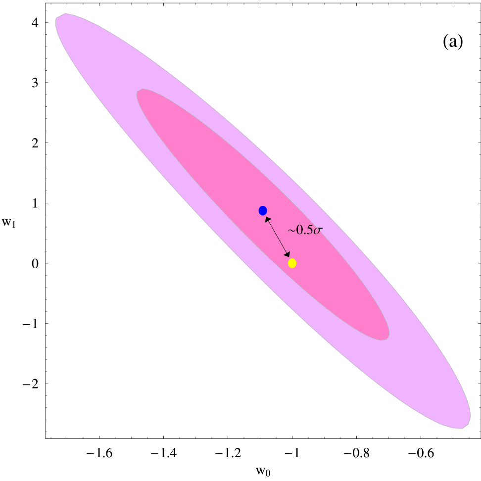
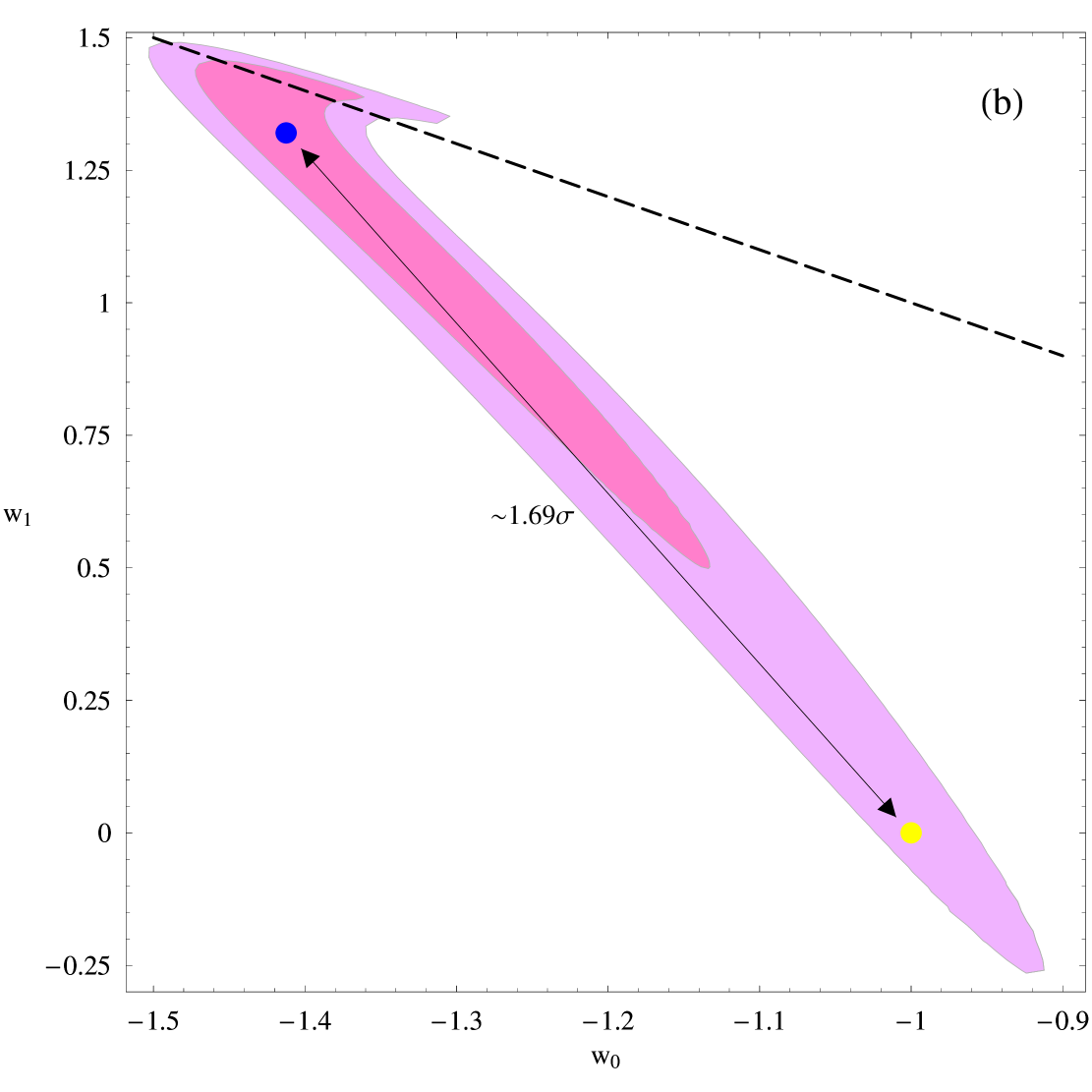
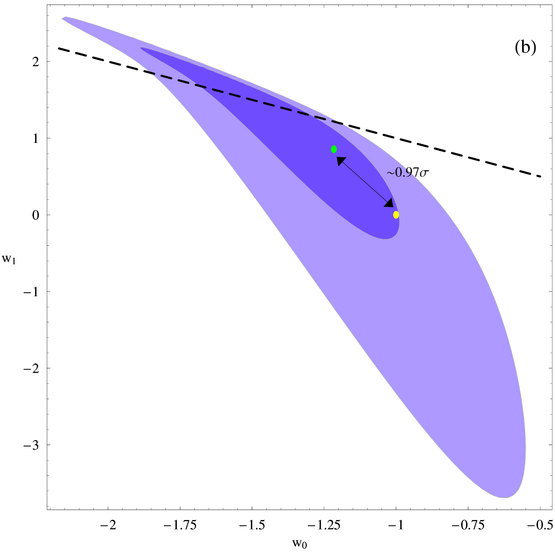
In Fig. 1 we show the $68.3\%$ and $95.4\%$ $\chi^{2}$ confidence contours in the $(w_{0},w_{1})$ parameter space for the two dataset categories (standard ruler and standard candle data) for $\Omega_{\rm 0m}=0.24$ and $\Omega_{b}=0.042$ (the best fit of the WMAP3 CMB data Spergel:2006hy ). Fig. 1a shows the $(w_{0},w_{1})$ contours obtained using SnIa data Davis:2007na (standard candles) while Fig. 1b shows the corresponding contours assuming CMB+BAO data Wang:2007mza ; Percival:2007yw (standard rulers). The blue dots correspond to the $(w_{0},w_{1})$ best fit, while the yellow dots correspond to $\Lambda$CDM $(w_{0},w_{1})=(-1,0)$. The distance in units of $\sigma$ ($\sigma$-distance $d_{\sigma}$) of the best fit to $\Lambda$CDM was found by converting $\Delta\chi^{2}=\chi^{2}_{\Lambda CDM}-\chi^{2}_{min}$ to $d_{\sigma}$ ie solving press92

$$1-\Gamma(1,\Delta\chi^{2}/2)/\Gamma(1)={\rm Erf}(d_{\sigma}/\sqrt{2})$$ (52)

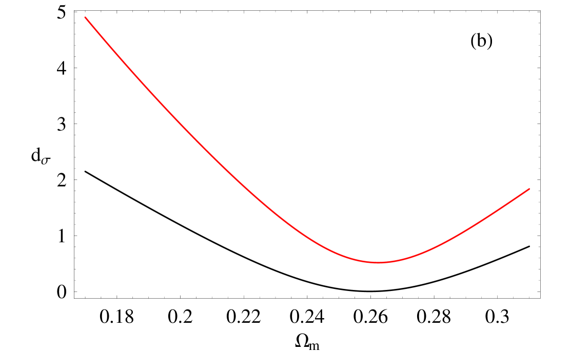
for $d_{\sigma}$ ($\sigma$-distance), where $\Delta\chi^{2}$ is the $\chi^{2}$ difference between the best-fit and $\Lambda$CDM and ${\rm Erf}()$ is the error function. Notice that $\Lambda$CDM is consistent at less than $1\sigma$ level according to the SnIa data ($d_{\sigma}^{SnIa}\simeq 0.5$ in Fig. 1a), while the corresponding consistency level reduces to $d_{\sigma}^{SR}\simeq 1.7\sigma$ for the standard ruler CMB+BAO data. This mild difference in trends between standard candles and standard rulers persists also for all values of $\Omega_{\rm 0m}$ in the $2\sigma$ range of WMAP3 best fit. This is demonstrated in Fig. 2 where we show the $\sigma$-distance $d_{\sigma}^{SR}$ superposed with $d_{\sigma}^{SnIa}$ as a function of $\Omega_{\rm 0m}$ for $\Omega_{b}=0.034$ (Fig. 2a), $\Omega_{b}=0.042$ (Fig. 2b) and $\Omega_{b}=0.049$ (Fig. 2c). These values of $\Omega_{b}$ span the $2\sigma$ range of the corresponding WMAP3 best fit. Notice that the $\sigma$-distance between best fit values and $\Lambda$CDM values is consistently larger when using standard ruler data (colored lines are consistently above black lines).

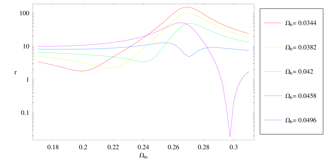
An alternative way to see this trend is to plot the ratios $r$ of the $\sigma$-distances defined as:

$$r(\Omega_{\rm 0m})\equiv\frac{d_{\sigma}^{SR}}{d_{\sigma}^{SnIa}}$$ (53)

These plots are shown in Fig. 3 for five values of $\Omega_{b}$ spanning the $2\sigma$ range of WMAP3. Notice that the colored lines are consistently above the line $r=1$ indicating that the $\sigma$-distance is found to be consistently larger when using standard ruler data. An exception to this rule is the case corresponding to high values of both $\Omega_{b}$ and $\Omega_{\rm 0m}$ set to values $2\sigma$ or more, away from their best fit (see magenta line corresponding to $\Omega_{b}=0.049$, for $\Omega_{\rm 0m}>0.29$).

Figure 6: The $68.3\%$ and $95.4\%$ $\chi^{2}$ confidence contours in the $(w_{0},w_{1})$ parameter space for the combined datasets SnIa+CMB+BAO for $\Omega_{\rm 0m}=0.24$. The blue dot corresponds to the $(w_{0},w_{1})$ best fit while the red dot to $\Lambda$CDM (-1,0).

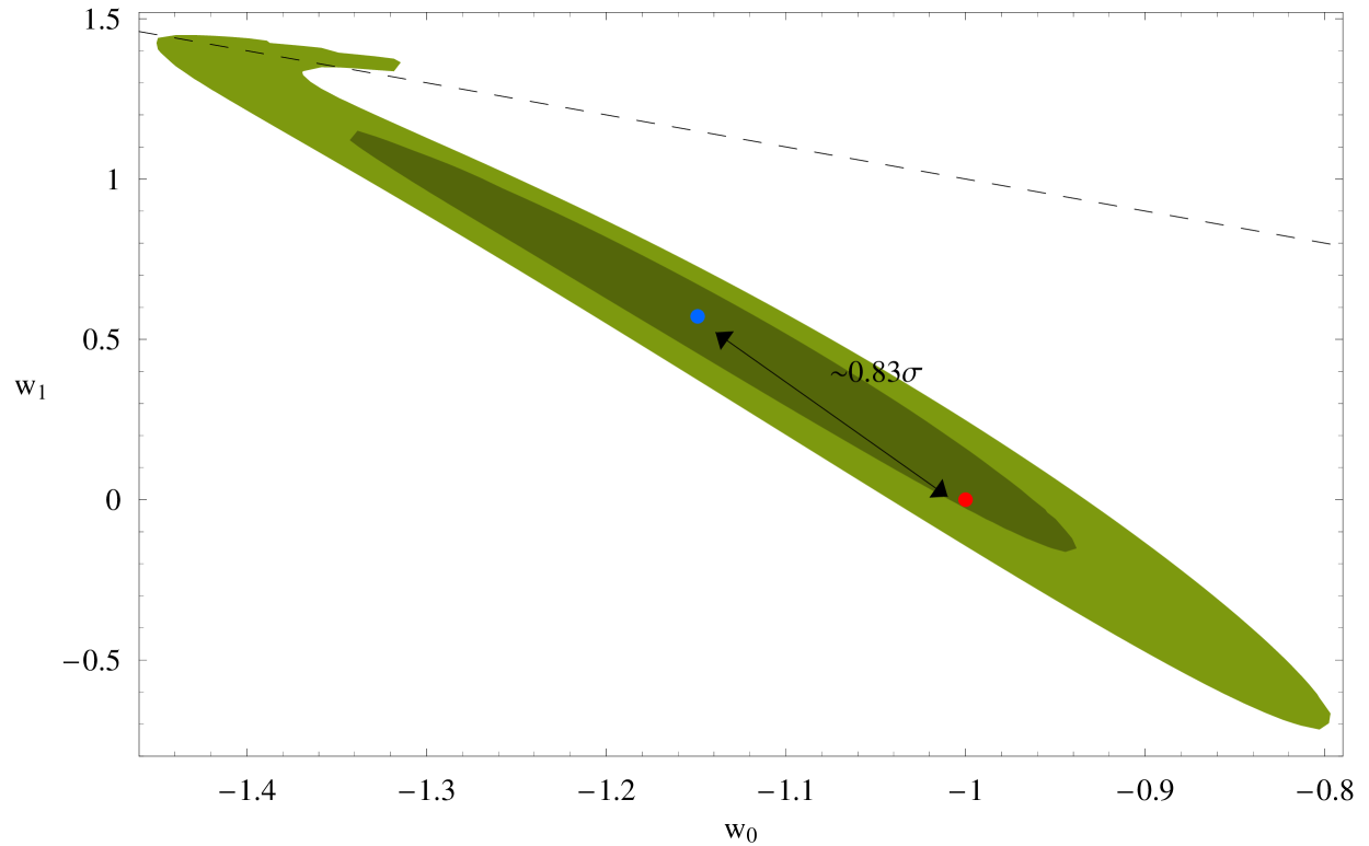
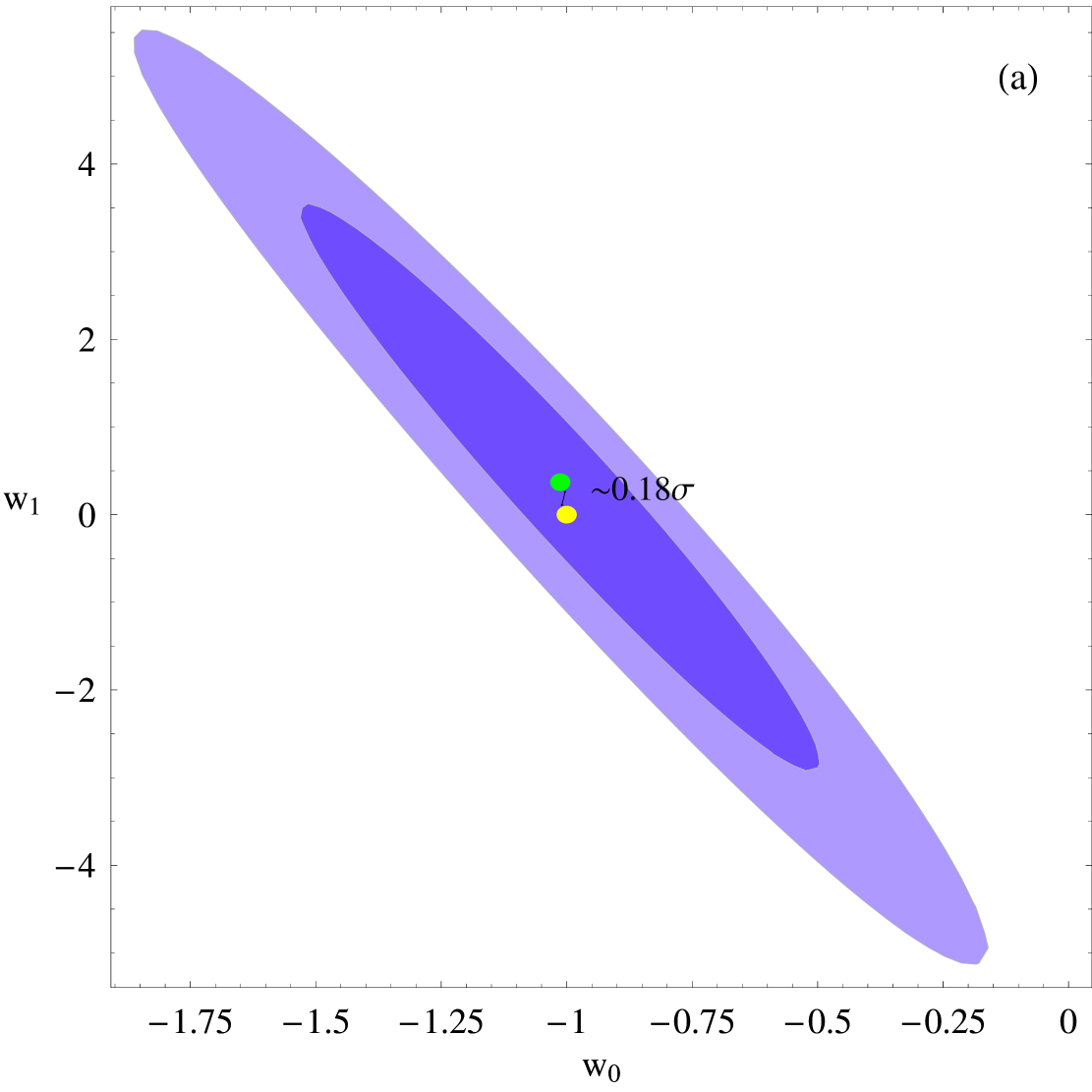
The above plots reveal a consistent trend of the standard ruler CMB+BAO data for a mild preference for crossing of the phantom divide line $w=-1$, while the recent SnIa data seem to favor $\Lambda$CDM. Figs. 4 and 5 show corresponding plots obtained using earlier data (SNLS Astier:2005qq vs CMB+BAO Wang:2006ts ; Eisenstein:2005su at $z=0.35$), where a similar consistent trend is observed.

An interesting feature of the contours of Fig. 1b is the deformation appearing for relatively large values of $w_{1}$. There is a simple way to understand this deformation. For $(w_{0},w_{1})$ parameter values satisfying $w_{0}+w_{1}\buildrel>\over{\sim}0$, the dark energy equation of state is approximately constant and positive at early times and therefore the corresponding dark energy density dominates over the matter density. As a result the Hubble expansion rate is significantly modified over the whole range from $z=0$ to $z_{CMB}$ and the corresponding integral of the shift parameters becomes very sensitive to parameter changes. The effect is even more significant for the shift parameter $l_{a}$ which involves the sound horizon $r_{s}$ in the denominator (see eq. (11). The sound horizon drops more dramatically than the shift parameter $R$ when the dark energy dominates at early times because the corresponding integral (12) depends only on the early time behavior of the expansion rate $H(a)$. This effect is demonstrated by plotting the $w_{0}+w_{1}=0$ line in Fig. 1b which coincides approximately with the region where the contour deformation starts. The same line is also plotted in Fig. 4b corresponding to early CMB+BAO dataEisenstein:2005su and involving only one shift parameter ($R$). In this case the deformation effect is milder because the z integral corresponding to $R$ spreads over a wide range of redshifts from $z=0$ to $z=1089$ and the effect of dark energy domination is somewhat smeared out.

We also construct the likelihood contours using the combined SnIa+CMB+BAO data for $\Omega_{\rm 0m}=0.24$ and $\Omega_{b}=0.042$ corresponding to the best fit WMAP3 parameter values. As expected, the $\sigma$-distance between best fit and $\Lambda$CDM is at about $1\sigma$, ie intermediate between the standard candle and standard ruler cases (see Fig. 6).

III Conclusions-Discussion

We have demonstrated that there is a systematic difference in trends between standard candle (SnIa) and standard ruler (CMB+BAO) data. The former data are significantly more consistent with $\Lambda$CDM than the later for practically all ($\Omega_{\rm 0m},\Omega_{b}$) parameter priors within the $2\sigma$ range of WMAP3. In fact, the standard ruler data demonstrate a mild preference for a best fit $w(z)$ that crosses the phantom divide line $w=-1$.

Figure 7: The constrains on $\eta(z)\equiv\frac{d_{L}(z)}{d_{A}(z)(1+z)^{2}}$ for $\Omega_{\rm 0m}=0.24$ in Fig. 7a and for $\Omega_{\rm 0m}=0.27$ in Fig. 7b. Clearly the anticipated value $\eta=1$ is within $1-2\sigma$ for both priors used.

This systematic difference in trends can be attributed to one of the following:

• Statistical Effects: There is an ($\Omega_{\rm 0m},\Omega_{b}$) parameter range where both datasets are consistent with each other and with $\Lambda$CDM at the $2\sigma$ level (see eg. Fig. 3b with $\Omega_{\rm 0m}\simeq 0.25$). Therefore, for these parameter values the two datasets are consistent with each other and with $\Lambda$CDM at the $1\sigma-2\sigma$ level and the trend we observe could well be a statistical fluctuation.

• Systematic-Physical Effects: As discussed in Ref. Bassett:2003vu distances based on standard candles and standard rulers should agree as long as three conditions are met: (1) photon number is conserved, (2) gravity is described by a metric theory and (3) photons are traveling on unique null geodesics. If at least one of these conditions is not met then equations (2) and (3) will lead to generically different forms for the Hubble expansion rate $H(z)$ due to the violation of the distance duality relation (5). For example, lensing of SnIa by compact objects, if not properly accounted for, would tend to violate condition (3) and induce artificial brightening of distant SnIa. Alternatively, photon number violation (due eg to photon mixing Mirizzi:2006zy ) would lead to artificial dimming of the SnIa.

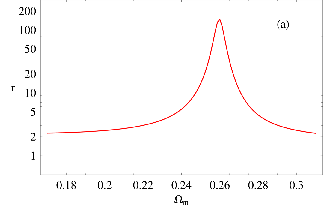
In order to investigate the possible existence of systematic physical effects, we have used our results to test the cosmic distance duality relation (5). In particular, we use our results for the best fit parameter values ($(w_{0},w_{1})$) and their error bars obtained from each dataset to derive constraints on the parameter $\eta(z)$. These constraints are shown in Fig. 7a for $\Omega_{\rm 0m}=0.24$ and in Fig. 7b $\Omega_{\rm 0m}=0.27$. Clearly, the anticipated value $\eta=1$ is within $2\sigma$ for both priors used. Assuming a prior of $\Omega_{\rm 0m}=0.24$ and taking an average value for $\eta(z)$ in the range $0<z<40$ (as for large enough $z$ $\eta(z)$ converges (see Fig 7)), yielding the value $\bar{\eta}=0.96\pm 0.07$ which is within $1\sigma$ from the anticipated value $\eta=1$. The consistency is somewhat reduced if we average over a more recent redshift range. In the range $1<z<2$ we find $\bar{\eta}=0.95\pm 0.025$ which is consistent with the anticipated value $\eta=1$ at the $2\sigma$ level. Similar results are obtained for other priors of $\Omega_{\rm 0m}$ within $2\sigma$ from the WMAP3 best fit. Therefore, despite the mild difference in trends between SnIa standard candles and CMB+BAO standard rulers, we find no statistically significant evidence for violation of the distance duality relation.

An interesting extension of this work would be the inclusion of more data from both categories. For example gamma ray bursts Meszaros:2006rc could also be included as standard candles and X-ray profiles of clusters Uzan:2004my or radio galaxies Daly:2007pp could be included as standard rulers in order to investigate if the mild difference in trends we have identified, persists in more general categories of data.

The Mathematica files with the numerical analysis of the paper can be found at http://leandros.physics.uoi.gr/rulcand/rulcand.htm

References

- (1) A. G. Riess et al. [Supernova Search Team Collaboration], Astrophys. J. 607, 665 (2004).
- (2) D. N. Spergel et al. [WMAP Collaboration], Astrophys. J. Suppl. 170, 377 (2007) [arXiv:astro-ph/0603449].
- (3) A. C. S. Readhead et al., Astrophys. J. 609, 498 (2004) [arXiv: astro-ph/0402359].
- (4) J. H. Goldstein et al., Astrophys. J. 599, 773 (2003) [arXiv:astro-ph/0212517].
- (5) R. Rebolo et al., MNRAS 353 747R (2004) [arXiv:astro-ph/0402466].
- (6) M. Tegmark et al. [SDSS Collaboration], Phys. Rev. D 69, 103501 (2004) [arXiv:astro-ph/0310723]
- (7) E. Hawkins et al., Mon. Not. Roy. Astron. Soc. 346, 78 (2003) [arXiv:astro-ph/0212375]
- (8) B. Boisseau, G. Esposito-Farese, D. Polarski and A. A. Starobinsky, Phys. Rev. Lett. 85, 2236 (2000) [arXiv:gr-qc/0001066]; E. Bertschinger, Astrophys. J. 648, 797 (2006) [arXiv:astro-ph/0604485]; J. P. Uzan, Gen. Rel. Grav. 39, 307 (2007) [arXiv:astro-ph/0605313]; J. P. Uzan and F. Bernardeau, Phys. Rev. D 64, 083004 (2001) [arXiv:hep-ph/0012011]; L. Perivolaropoulos, JCAP 0510, 001 (2005) [arXiv:astro-ph/0504582]; R. Caldwell, A. Cooray and A. Melchiorri, Phys. Rev. D 76, 023507 (2007) [arXiv:astro-ph/0703375]; B. Jain and P. Zhang, arXiv:0709.2375 [astro-ph]; S. Nesseris and L. Perivolaropoulos, Phys. Rev. D 73, 103511 (2006) [arXiv:astro-ph/0602053]; S. Wang, L. Hui, M. May and Z. Haiman, Phys. Rev. D 76, 063503 (2007) [arXiv:0705.0165 [astro-ph]]; S. Tsujikawa, Phys. Rev. D 76, 023514 (2007) [arXiv:0705.1032 [astro-ph]]; A. F. Heavens, T. D. Kitching and L. Verde, arXiv:astro-ph/0703191; S. Nesseris and L. Perivolaropoulos, Phys. Rev. D 75, 023517 (2007) [arXiv:astro-ph/0611238]; J. P. Uzan, Phys. Rev. D 59, 123510 (1999) [arXiv:gr-qc/9903004]; V. Sahni and Y. Shtanov, JCAP 0311, 014 (2003) [arXiv:astro-ph/0202346].
- (9) A. Vikman, Phys. Rev. D 71, 023515 (2005) [arXiv:astro-ph/0407107].
- (10) J. Benjamin et al., arXiv:astro-ph/0703570; C. Shapiro and S. Dodelson, Phys. Rev. D 76, 083515 (2007) [arXiv:0706.2395 [astro-ph]]; L. Amendola, M. Kunz and D. Sapone, arXiv:0704.2421 [astro-ph]; A. Refregier et al., arXiv:astro-ph/0610062.
- (11) A. J. S. Hamilton, arXiv:astro-ph/9708102; E. V. Linder, arXiv:0709.1113 [astro-ph]; S. Nesseris and L. Perivolaropoulos, arXiv:0710.1092 [astro-ph]; C. Di Porto and L. Amendola, arXiv:0707.2686 [astro-ph]; Y. Wang, arXiv:0710.3885 [astro-ph].
- (12) A. G. Riess et al., arXiv:astro-ph/0611572.
- (13) T. M. Davis et al., Astrophys. J. 666, 716 (2007) [arXiv:astro-ph/0701510].
- (14) P. Astier et al., arXiv:astro-ph/0510447.
- (15) P. Meszaros, Rept. Prog. Phys. 69, 2259 (2006) [arXiv:astro-ph/0605208]; E. W. Liang and B. Zhang, Astrophys. J. 633, 611 (2005) [arXiv:astro-ph/0504404]; D. Lazzati, G. Ghirlanda, G. Ghisellini, L. Nava, C. Firmani, B. Morsony and M. C. Begelman, AIP Conf. Proc. 836 (2006) 513 [arXiv:astro-ph/0602216]; D. Hooper and S. Dodelson, Astropart. Phys. 27, 113 (2007) [arXiv:astro-ph/0512232]; F. Y. Wang, Z. G. Dai and Z. H. Zhu, arXiv:0706.0938 [astro-ph].
- (16) M. Bonamente, M. K. Joy, S. J. La Roque, J. E. Carlstrom, E. D. Reese and K. S. Dawson, arXiv:astro-ph/0512349; L. Samushia, G. Chen and B. Ratra, arXiv:0706.1963 [astro-ph].
- (17) J. P. Uzan, N. Aghanim and Y. Mellier, Phys. Rev. D 70, 083533 (2004) [arXiv:astro-ph/0405620]; F. De Bernardis, E. Giusarma and A. Melchiorri, Int. J. Mod. Phys. D 15, 759 (2006) [arXiv:gr-qc/0606029].
- (18) R. A. Daly, M. P. Mory, C. P. O’Dea, P. Kharb, S. Baum, E. J. Guerra and S. G. Djorgovski, arXiv:0710.5112 [astro-ph]; S. Podariu, R. A. Daly, M. P. Mory and B. Ratra, Astrophys. J. 584, 577 (2003) [arXiv:astro-ph/0207096].
- (19) S. Nesseris and L. Perivolaropoulos, JCAP 0701, 018 (2007) [arXiv:astro-ph/0610092].
- (20) S. Nesseris and L. Perivolaropoulos, Phys. Rev. D 72, 123519 (2005) [arXiv:astro-ph/0511040].
- (21) S. Nesseris and L. Perivolaropoulos, JCAP 0702, 025 (2007) [arXiv:astro-ph/0612653].
- (22) W. M. Wood-Vasey et al. [ESSENCE Collaboration], Astrophys. J. 666, 694 (2007) [arXiv:astro-ph/0701041]; G. Miknaitis et al., arXiv:astro-ph/0701043;
- (23) P. S. Corasaniti and A. Melchiorri, arXiv:0711.4119 [astro-ph]; O. Elgaroy and T. Multamaki, Astron. Astrophys. 471, 65 (2007) arXiv:astro-ph/0702343.
- (24) U. Alam, V. Sahni and A. A. Starobinsky, JCAP 0702, 011 (2007) [arXiv:astro-ph/0612381].
- (25) Y. Wang and P. Mukherjee, arXiv:astro-ph/0703780.
- (26) W. J. Percival, S. Cole, D. J. Eisenstein, R. C. Nichol, J. A. Peacock, A. C. Pope and A. S. Szalay, arXiv:0705.3323 [astro-ph].
- (27) E. V. Linder, Phys. Rev. D 68, 083503 (2003) [arXiv:astro-ph/0212301].
- (28) M. Chevallier and D. Polarski, Int. J. Mod. Phys. D 10, 213 (2001) [arXiv:gr-qc/0009008].
- (29) W. Hu, M. Fukugita, M. Zaldarriaga and M. Tegmark, Astrophys. J. 549, 669 (2001) [arXiv:astro-ph/0006436]; W. J. Percival et al. [The 2dFGRS Team Collaboration], Mon. Not. Roy. Astron. Soc. 337, 1068 (2002) [arXiv:astro-ph/0206256].
- (30) S. Nesseris and L. Perivolaropoulos, Phys. Rev. D 70, 043531 (2004) [arXiv:astro-ph/0401556].
- (31) W. H. Press et. al., “Numerical Recipes”, Cambridge University Press (1994).
- (32) Y. Wang and P. Mukherjee, Astrophys. J. 650, 1 (2006) [arXiv:astro-ph/0604051].
- (33) D. J. Eisenstein et al. [SDSS Collaboration], Astrophys. J. 633, 560 (2005) [arXiv:astro-ph/0501171].
- (34) B. A. Bassett and M. Kunz, Phys. Rev. D 69, 101305 (2004) [arXiv:astro-ph/0312443].
- (35) A. Mirizzi, G. G. Raffelt and P. D. Serpico, arXiv:astro-ph/0607415; C. Burrage, arXiv:0711.2966.