Unsupervised and semi-supervised clustering by message passing:
Soft-constraint affinity propagation

Abstract

Soft-constraint affinity propagation (SCAP) is a new statistical-physics based clustering technique SCAP . First we give the derivation of a simplified version of the algorithm and discuss possibilities of time- and memory-efficient implementations. Later we give a detailed analysis of the performance of SCAP on artificial data, showing that the algorithm efficiently unveils clustered and hierarchical data structures. We generalize the algorithm to the problem of semi-supervised clustering, where data are already partially labeled, and clustering assigns labels to previously unlabeled points. SCAP uses both the geometrical organization of the data and the available labels assigned to few points in a computationally efficient way, as is shown on artificial and biological benchmark data.

1 Introduction

Clustering is a very important problem in data analysis JAIN ; DUDA . Starting from a set of data points, one tries to group data such that points in one cluster are more similar in between each other than points in different clusters. The hope is that such a grouping unveils common functional characteristics. As an example, one of the currently most important application fields for clustering is the informatical analysis of biological high-throughput data, as given e.g. by gene expression data. Different cell states result in different expression patterns.

If data are organized in a well-separated way, one can use one of the many unsupervised clustering methods to divide them into classes JAIN ; DUDA ; but if clusters overlap at their borders or if they have involved shapes, these algorithms in general face problems. However, clustering can still be achieved using a small fraction of previously labeled data (training set), making the clustering semi-supervised BOOK ; DOMANY2 . While designing algorithms for semi-supervised clustering, one has to be careful: They should efficiently use both types of information provided by the geometrical organization of the data points as well as the already assigned labels.

In general there is not only one possible clustering. If one goes to a very fine scale, each single data point can be considered its own cluster. On a very rough scale, the whole data set becomes a single cluster. These two extreme cases may be connected by a full hierarchy of cluster-merging events.

This idea is the basis of the oldest clustering method, which still is amongst the most popular one: hierarchical agglomerative clustering SOKAL ; JOHNSON . It starts with clusters being isolated points, and in each algorithmic step the two closest clusters are merged (with the cluster distance given, e.g., by the minimal distance between pairs of cluster elements), until only one big cluster appears. This process can be visualized by the so-called dendrogram, which shows clearly possible hierarchical structures. The strong point of this algorithm is its conceptual clarity connected to an easy numerical implementation. Its major problem is that it is a greedy and local algorithm, no decision can be reversed.

A second traditional and broadly used clustering method is K-means clustering MCQUEEN . In this algorithm, one starts with a random assignment of data points to $K$ clusters, calculates the center of mass of each cluster, reassigns points to the closest cluster center, recalculates cluster centers etc., until the cluster assignment is converged. This method is a very efficiently implementable method, but it shows a strong dependence on the initial condition, getting trapped by local optima. So the algorithm has to be rerun many times to produce reliable clusterings, and the algorithmic efficiency is decreased. Further on $K$-means clustering assumes spherical clusters, elongated clusters tend to be divided artificially in sub-clusters.

A first statistical-physics based method is super-paramagnetic clustering DOMANY1 ; DOMANY2 . The idea is the following: First the network of pairwise similarities becomes preprocessed, only links to the closest neighbors are kept. On this sparsified network a ferromagnetic Potts model is defined. In between the paramagnetic high-temperature and the ferromagnetic low-temperature phase a super-paramagnetic phase can be found, where already large clusters tend to be aligned. Using Monte-Carlo simulations, one measures the pairwise probability for any two points to take the same value of their Potts variables. If this probability is large enough, these points are identified to be in the same cluster. This algorithm is very elegant since it does not assume any cluster number of structure, nor uses greedy methods. Due to the slow equilibration dynamics in the super-paramagnetic regime it needs, however, the implementation of sophisticated cluster Monte-Carlo algorithms. Note that also super-paramagnetic clusterings can be obtained by message passing techniques, but these require an explicit breaking of the symmetry between the values of the Potts variables to give non-trivial results.

Also in the last years, many new clustering methods are being proposed. One particularly elegant and powerful method is affinity propagation (AP) FREY , which gave also the inspiration to our algorithm. The approach is slightly different: Each data point has to select an exemplar in between all other data points. This shall be done in a way to maximize the overall similarity between data points and exemplars. The selection is, however, restricted by a hard constraint: Whenever a point is chosen as an exemplar by somebody else, it is forced to be also its own self-exemplar. Clusters are consequently given as all points with a common exemplar. The number of clusters is regulated by a chemical potential (given in form of a self-similarity of data points), and good clusterings are identified via their robustness with respect to changes in this chemical potential. The computational hard task to optimize the overall similarity under the hard constraints is solved via message passing YEDIDIA ; MAXSUM , more precisely via belief propagation, which are equivalent to the Bethe-Peierls approximation / the cavity method in statistical physics MezardParisi ; MyBook . Despite the very good performance on test data, also AP has some drawbacks: It assumes again more or less spherical clusters, which can be characterized by a single cluster exemplar. It does not allow for higher order pointing processes. A last concern is the robustness: Due to the hard constraint, the change of one single exemplar may result in a large avalanche of other changes.

The aim of soft-constraint affinity propagation (SCAP) is to use the strong points and ideas of affinity propagation – the exemplar choice fulfilling a global optimization principle, the computationally efficient implementation via message-passing techniques – but curing the problems arising from the hard constraints. In SCAP we have proposed a first version of this algorithm, and have shown that on gene-expression data it is very powerful. In this article, we propose a simplified version which is more efficient. Finally we show that SCAP also allows for a particularly elegant generalization to the semi-supervised case, i.e. to the inclusion of partially labeled data. As shown in some artificial and biological benchmark data, the partial labeling allows to extract the correct clustering even in cases where the unsupervised algorithm fails.

The plan of the paper is the following: After this Introduction, we present in Sec. 2 the clustering problem and the derivation of SCAP, and we discuss time- and memory-efficient implementations which become important in the case of huge data sets. In Sec. 3 we test the performance of SCAP on artificial data with clustered and hierarchical structures. Sec. 4 is dedicated to the generalization to semi-supervised clustering, and we conclude in the final Sec. 5.

2 The algorithm

2.1 Formulation of the problem

The basic input to SCAP are pairwise similarities $S(\mu,\nu)$ between any two data points $\mu,\nu\in\{1,...,N\}$. In many cases, these similarities are given by the negative (squared) Euclidean distances between data points or by some correlation measure (as Pearson correlations) between data points. In principle they need not even to be symmetric in $\mu$ and $\nu$, as they might represent conditional dependencies between data points. The choice of the correct similarity measure will for sure influence the quality and the details of the clusterings found by SCAP, it depends on the nature of the data which shall be clustered. Here we assume therefore the similarities to be given.

The main idea of SCAP is that each data point $\mu$ selects some other data point $\nu$ as its exemplar, i.e. as some reference point for itself. The exemplar choice is therefore given by a mapping

$${\mathbf{c}}:\ \ \{1,...,N\}\ \mapsto\ \{1,...,N\}$$ (1)

where, in difference to the original AP and the previous version of SCAP, no self-exemplars are allowed:

$$\forall\mu\in\{1,...,N\}:\ \ c_{\mu}\neq\mu\ .$$ (2)

The mapping ${\mathbf{c}}$ defines a directed graph with links going from data points to their exemplars, and clusters in this approach correspond to the connected components of (an undirected version) this graph.

The aim in constructing ${\mathbf{c}}$ is to minimize the Hamiltonian, or cost function,

$${\cal H}({\mathbf{c}})=-\sum_{\mu=1}^{N}S(\mu,c_{\mu})\ +\ p\ {\cal N}_{c}\ ,$$ (3)

with ${\cal N}_{c}$ being the number of distinct selected exemplars. This Hamiltonian consists of two parts: The first one is the negative sum of the similarities of all data points to their exemplars, so the algorithm tries to maximize this accumulated similarity. However, this term alone would lead to a local greedy clustering where each data point chooses its closest neighbor as an exemplar. The resulting clustering would contain ${\cal O}(N)$ clusters, so increasing the amount of data would lead to more instead of better defined clusters. The second term serves to compactify the clusters: $\chi_{\mu}$ is one iff $\mu$ is an exemplar, so each exemplar has to pay a penalty $p$. Since this penalty does not depend on how many data points actually choose $\mu$ as their exemplar (the in-degree of $\mu$), mappings ${\bf c}$ with few exemplars of high in-degree are favored, leading to more compact clusters. In this way, the parameter $p$ controls the cluster number, robust clusterings are recognized due to their stability under changing $p$. Since the cluster number is not fixed a priori, SCAP also recognizes successfully a hierarchical cluster organization.

For later convenience we express the exemplar number as

$${\cal N}_{c}=\sum_{\mu=1}^{N}\chi_{\mu}({\mathbf{c}})\ ,$$ (4)

using an indicator function

$$\chi_{\mu}({\mathbf{c}})=\left\{\begin{array}[]{ccl}1&&{\rm if}\ \exists\nu:\ c_{\nu}=\mu\\ 0&&{\rm else}\end{array}\right.$$ (5)

which denotes the soft local constraint acting on each data point.

Note that this problem setting is slightly different from the one used in the first derivation of SCAP in SCAP . There self-exemplars were allowed, and only selecting an exemplar which was not a self-exemplar led to the application of the penalty $p$. The number of self-exemplars itself was coupled to a second parameter, the self-similarity. In SCAP we already found that the best results were obtained for very small self-similarities. Actually the algorithm presented here can be obtained from the previous formulation by explicitly sending all self-similarities $S(\mu,\mu)\to-\infty$. The resulting formulation is easier both in implementation and interpretation since it does not include self-messages.

2.2 Derivation of the algorithm

The exact minimization of this Hamiltonian is a computationally hard problem: There are $(N-1)^{N}$ possible configurations $c$ to be tested, resulting in a potentially super-exponential running time of any exact algorithm. We therefore need efficient heuristic approaches which, even if not guaranteeing to find the true optimum, are algorithmically feasible.

An approach related to the statistical physics of disordered systems is the implementation of message-passing techniques, more precisely of the belief propagation algorithm YEDIDIA ; MAXSUM . The latter is equivalent to an algorithmic interpretation of the Bethe-Peierls approximation in statistical physics: Instead of solving exactly the thermodynamics of the problem, we use a refined mean-field method.

To do so, we first introduce a formal inverse temperature $\beta$ and the corresponding Gibbs weight

$${\mathbf{P}}({\mathbf{c}})\sim\exp\{-\beta{\cal H}({\mathbf{c}})\}\ .$$ (6)

The temperature will be sent to zero at the end of the calculations, to obtain a weight concentrated completely in the ground states of ${\cal H}$. In principle one should optimize ${\mathbf{P}}({\mathbf{c}})$ with respect to the joint choice of all exemplars, we will replace this by the independent optimization of all marginal single-variable probabilities. We thus need to estimate the probabilities

$$P_{\mu}(c_{\mu})=\sum_{\{c_{\nu};\nu\neq\mu\}}{\mathbf{P}}({\mathbf{c}})$$ (7)

which in principle contain a sum over the $(N-1)^{N-1}$ configurations of all other variables. From this marginal probability we can define an exemplar choice as

$$c_{\mu}^{\star}=\underset{c_{\mu}}{\rm argmax}\lim_{\beta\to\infty}P_{\mu}(c_{\mu})\ .$$ (8)

Note that this becomes the correct global minimum of ${\mathbf{P}}$ if the latter is non-degenerate which is a reasonable assumption in the case of real-valued similarities $S(\mu,\nu)$.

We want to estimate these marginal distributions using belief propagation, or equivalently the Bethe-Peierls approximation. For doing so, we first represent the problem by its factor graph as given in Fig. 1. The variables are represented by circular variable nodes, the constraints $\chi_{\mu}$ by square factor nodes. Due to the special structure of the problem, every variable node corresponds to exactly one factor node. Each factor node is connected to all variable nodes which are contained in the constraint (which are all but the one corresponding to the factor node). The similarities act locally on variable nodes, they can be interpreted as $(N-1)$-dimensional local vector fields.

Figure 1: Factor graph for SCAP: Circles denote variable nodes, related to the variables $c_{\mu}$, whereas squares denote the constraints $\chi_{\mu}$. A link is drawn whenever a variable compares in a constraint, i.e. all variable nodes $\nu\neq\mu$ are connected to factor node $\chi_{\mu}$. Similarities act as external $(N-1)$-dimensional fields on the variables. The figure also displays the two message types send from variables to constraints and back.

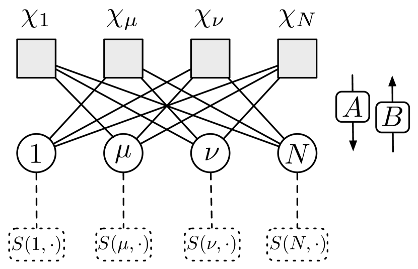
Belief propagation works via the exchange of messages between variable and factor nodes. Let us denote first $A_{\mu\to\nu}(c_{\nu})$ the message sent from constraint $\mu$ to variable $\nu$, measuring the probability that $\mu$ forces $\nu$ to select $c_{\nu}$ as its exemplar. Second we introduce $B_{\nu\to\mu}(c_{\nu})$ as the probability that variable $\nu$ would choose $c_{\nu}$ as its exemplar without the presence of constraint $\mu$. Than we can write down closed iterative equations, called belief-propagation equations,

$$A_{\mu\to\nu}(c_{\nu}) \propto \prod_{\lambda\neq\mu,\nu}\left[\sum_{c_{\lambda}}B_{\lambda\to\mu}(c_{\lambda})\right]\exp\{-\beta\,p\,\chi_{\mu}({\mathbf{c}})\}$$

$$B_{\mu\to\nu}(c_{\mu}) \propto \prod_{\lambda\neq\mu,\nu}A_{\lambda\to\mu}(c_{\mu})\exp\{\beta\,S(\mu,c_{\mu})\}\ .$$ (9)

We see that the message $A_{\mu\to\nu}$ from constraint $\mu$ to variable $\nu$ depends on the choices all other variables would take without constraint $\mu$, times the Gibbs weight of constraint $\chi_{\mu}$. The message $B_{\mu\to\nu}$ from variable $\mu$ to constraint $\nu$ depends on the messages from all other constraints to $\mu$, and the local field $\vec{S}$ on $\mu$. The approximate character of belief propagation stems from the fact that the joint distributions over all neighboring variables is taken to be factorized into single variable quantities. Having solved these equations we can easily estimate the true marginal distributions

$$P_{\mu}(c_{\mu})\propto\prod_{\lambda\neq\mu}A_{\lambda\to\mu}(c_{\mu})\exp\{\beta\,S(\mu,c_{\mu})\}$$ (10)

which are the central quantities we are looking for.

However, looking at the first of Eqs. (2.2), we realize that it still contains the super-exponential sum. Further on, we need a memory space of ${\cal O}(N^{3})$ to store all these messages, which is practical only for small and intermediate data sets. This problem can be resolved exactly by realizing that $A_{\mu\to\nu}(c_{\mu})$ takes only two values for fixed $\mu$ and $\nu$, namely $A_{\mu\to\nu}(\mu)$ and $A_{\mu\to\nu}(c\neq\mu)$ . We therefore introduce the reduced messages

$$\tilde{A}_{\mu\to\nu} = \frac{A_{\mu\to\nu}(\mu)}{A_{\mu\to\nu}(c\neq\mu)}$$

$$\tilde{B}_{\mu\to\nu} = B_{\mu\to\nu}(\nu)\ .$$ (11)

After a little book-keeping work to consider all possible cases, the sums in Eqs. (2.2,10) can be performed analytically resulting in a set of equivalent relations

$$\tilde{A}_{\mu\to\nu} = \left[1+(e^{\beta p}-1)\prod_{\lambda\neq\mu,\nu}(1-\tilde{B}_{\lambda\to\mu})\right]^{-1}$$

$$\tilde{B}_{\mu\to\nu} = \left[1+\sum_{\lambda\neq\mu,\nu}e^{\beta S(\mu,\lambda)-\beta S(\mu,\nu)}\tilde{A}_{\lambda\to\mu}\right]^{-1}$$

$$P_{\mu}(c) = \frac{e^{\beta\,S(\mu,c)}\tilde{A}_{c\to\mu}}{\sum_{\lambda\neq\mu}e^{\beta\,S(\mu,\lambda)}\tilde{A}_{\lambda\to\mu}}\ .$$ (12)

These equations are the finite-temperature SCAP equations. Note that the complexity of evaluating the first line is decreased from ${\cal O}(N^{N})$ to ${\cal O}(N)$ and therefore feasible even for very large data sets. Also the memory requirements are decreased to ${\cal O}(N^{2})$. As we will see later on, a clever implementation will, in particular in the zero-temperature limit, further decrease time- and space-complexity.

2.3 SCAP in the zero-temperature limit

Even if Eqs. (2.2) are already relatively simple, the zero temperature limit of these equations becomes even simpler and bears a very intuitive interpretation. To achieve this limit, we have to transform the variables in the equations from probabilities to local fields, and introduce

$$a_{\mu\to\nu} = \frac{1}{\beta}\ln\tilde{A}_{\mu\to\nu}$$

$$r_{\mu\to\nu} = \frac{1}{\beta}\ln\frac{\tilde{B}_{\mu\to\nu}}{1-\tilde{B}_{\mu\to\nu}}\ .$$ (13)

We call $a_{\mu\to\nu}$ the availability of $\mu$ to be an exemplar for $\nu$, whereas $r_{\mu\to\nu}$ measures the request of $\mu$ to point $\nu$ to be its exemplar. Using the fact that sums over various exponential terms in $\beta$ are dominated by the maximum term, we readily conclude

$$r_{\mu\to\nu} = S(\mu,\nu)-{\rm max}_{\lambda\neq\mu,\nu}\left[S(\mu,\lambda)+a_{\lambda\to\mu}\right]$$

$$a_{\mu\to\nu} = {\rm min}\left[0,\,-p+\sum_{\lambda\neq\mu,\nu}{\rm max}(0,\,r_{\lambda\to\mu})\right]$$ (14)

to hold for these two fields.

These equations have a very nice and intuitive interpretation in terms of a social dynamics of exemplar selection. The system tries to maximize its overall similarity (or gain) which is the sum over all similarities between data points and their exemplars, but each exemplar has to pay a penalty $p$. Therefore each data point $\mu$ sends requests to all their neighbors $\nu$, which are composed by two contributions: The similarity to the neighbor itself, minus the maximum over all similarities to the other points $\lambda\neq\mu,\nu$ - the latter already being corrected for by the availability of the other points to be an exemplar. Now, data points $\mu$ communicate their availability to be an exemplar for any other data point $\nu$. For doing so, they sum up all positive requests from further points $\lambda\neq\mu,\nu$, and compare it to the penalty they have to pay in case they accept to be an exemplar. If the accumulated positive requests are bigger than the penalty, $\mu$ agrees right away to be the exemplar for $\nu$. If on the other hand the penalty is larger than the requests, $\mu$ communicates to $\nu$ the difference - so the answer is not a simple “no” but is weighed. Point $\nu$ should overcome this difference with its similarity.

Consequently the exemplar choice of $\mu$ happens via the selection of the neighbor $\nu$ who has the highest value of the similarity corrected by the availability of $\nu$ for $\mu$, i.e. we have

$$c_{\mu}^{\star}=\underset{\nu}{\rm argmax}\left[S(\mu,\nu)+a_{\nu\to\mu}\right]\ .$$ (15)

Eqs. (2.3,15) are called soft-constraint affinity propagation. They can be solved by first iteratively solving (2.3), and then plugging the solution into (15). The next two sub-sections will show how this can be done in a time- and memory efficient way.

2.4 Time-efficient implementation

The iterative solution of Eqs. (2.3) can be implemented in the following way:

1. Define the similarity $S(\mu,\nu)$ for each set of data points. Choose the values of the self-similarity $\sigma$ and of the constraint strength $p$. Initialize all $a(\mu,\nu)=r(\mu,\nu)=0$

2. For all $\mu\in\{1,...,N\}$, first update the $N$ requests $r_{\mu\to\nu}$ and then the $N$ availabilities $a_{\mu\to\nu}$, using Eqs. (2.3).

3. Identify the exemplars $c_{\mu}^{\star}$ by looking at the maximum value of $S(\mu,\nu)+a_{\nu\to\mu}$ for given $\mu$, according to Eq. (15).

4. Repeat steps 2-3 till there is no change in exemplars for a large number of iterations (we used 10-100 iterations). If not converged after $T_{max}$ iterations (typically 100-1000), stop the algorithm.

Three notes are necessary at this point:

• Step 3 is formulated as a sequential update: For each data point $\mu$, all outgoing responsibilities and then all incoming availabilities are updated before moving to the next data point. In numerical experiments this was found to converge faster and in a larger parameter range than the damped parallel update suggested by Frey and Dueck in FREY . The actual implementation uses a random sequential update, i.e. each time step 3 is performed, we generate a random permutation of the order of the $\mu\in\{1,...,N\}$.

• The naive implementation of the update equations (2.3) requires ${\cal O}(N^{2})$ updates, each one of computational complexity ${\cal O}(N)$. A factor $N$ can be gained by first computing the unrestricted max and sum once for a given $\mu$, and then implying the restriction only inside the internal loop over $\nu$. Like this, the total complexity of a global update is ${\cal O}(N^{2})$ and thus feasible even for very large data sets.

• Belief propagation on loopy graphs is not guaranteed to converge. We observe, that even in cases where the messages do not converge to a fixed point but go on fluctuating, the exemplar choice converges. In our algorithm, we therefore apply frequently the stationarity of ${\mathbf{c}}^{\star}$ as a weaker convergence criterion than message convergence.

2.5 Memory-efficient implementation

Another problem of SCAP can be its memory size, Eqs. (2.3) require the storage of three arrays of size $N^{2}$. This can be a problem if we consider very large data sets. A particularly important example are gene-expression data, which may contain more than 30,000 genes. If one wants to cluster these genes to identify coexpressed gene groups, the required memory size becomes fastly much larger than the working memory of a standard desktop computer, restricting the size of data sets to approximately $N<10^{4}$.

However, this problem can be resolved in the zero-temperature equations by not storing messages and similarities (which are indexed by two numbers) but only site quantities (which are indexed by a single number) reducing thus the memory requirements to ${\cal O}(N)$. This allows to treat even the largest available data sets efficiently with SCAP.

As a first step, we note that in most cases data are multi-dimensional. For example in gene expression data, a typical data sets contains about 100 micro-arrays measuring simultaneously 5,000-30,000 genes. If we want to cluster arrays, for sure a direct implementation of Eqs. (2.3,15) is best. In particular only the similarities are needed actively instead of the initial data points. If, on the other hand, we want to clusterize genes, it is more efficient to calculate similarities whenever needed from the original data, instead of memorizing the huge similarity matrix.

Once this is implemented, we can also get rid of the messages $a_{\mu\to\nu}$ and $r_{\mu\to\nu}$. First we introduce

$$h_{\mu}^{(1)} = \underset{\lambda\neq\mu}{\rm max}\left[S(\mu,\lambda)+a_{\lambda\to\mu}\right]$$

$$c_{\mu}^{(1)} = \underset{\lambda\neq\mu}{\rm argmax}\left[S(\mu,\lambda)+a_{\lambda\to\mu}\right]$$

$$h_{\mu}^{(2)} = \underset{\lambda\neq\mu,c_{\mu}^{(1)}}{\rm max}\left[S(\mu,\lambda)+a_{\lambda\to\mu}\right]\ .$$ (16)

These quantities, together with the similarities (directly calculated from the original data) are sufficient to express all requests,

$$r_{\mu\to\nu}=S(\mu,\nu)-h_{\mu}^{(1)}+\left(h_{\mu}^{(1)}-h_{\mu}^{(2)}\right)\,\delta_{\nu,c_{\mu}^{(1)}}$$ (17)

with $\delta_{\cdot,\cdot}$ being the Kronecker-symbol. A similar step can be done for the availabilities. We introduce

$$u_{\mu}=\sum_{\lambda\neq\mu}{\rm max}(0,\,r_{\lambda\to\mu})$$ (18)

and express the availability as

$$a_{\mu\to\nu} = {\rm min}\Big{[}0,\,-p+u_{\mu}$$

$$\left.-{\rm max}\left\{0,\,S(\nu,\mu)-h_{\nu}^{(1)}+\left(h_{\nu}^{(1)}-h_{\nu}^{(2)}\right)\,\delta_{\mu,c_{\nu}^{(1)}}\right\}\right]$$

Note that after convergence we have trivially

$$c_{\mu}^{\star}=c_{\mu}^{(1)}$$ (20)

for all $\mu\in\{1,...,N\}$.

In this way, instead of storing $S(\mu,\nu)$, $a_{\mu\to\nu}$ and $r_{\mu\to\nu}$ we have to store only the data, $h_{\mu}^{(1,2)},\ c_{\mu}^{(1)}$ and $u_{\mu}$. The largest array is the data set itself, all other memorized quantities require much less size. For large data sets, in this way the memory usage becomes much more efficient. Even if the algorithm requires more steps to be executed (similarities and messages have to be computed whenever they are needed, instead of a single time in each update step), the more efficient memory usage leads to strongly decreased running times.

3 Artificial data

In SCAP we have shown that SCAP is able to successfully cluster biological data coming from gene-expression arrays. This is true also for the simplified version derived in the present work. Here we aim, however, at a more theoretical analysis on artificial data which will bring light into some characteristics of SCAP, and which will allow for a more detailed comparison to the performance of AP as defined originally in FREY . To start with, we first consider numerically data having only one level of clustering, later on we extend this study to more than one level of clusters, i.e. to a situation where clusters of data points itself are organized in larger clusters.

3.1 One cluster level

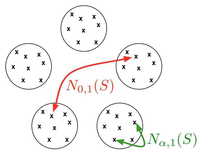
The first step is very simple: We define an artificial data set having only one level of clustering. We therefore start with $N$ data points which are divided into $q$ equally sized subsets. For each pair inside such a subset we draw randomly and independently a similarity from a Gaussian of mean $\alpha$ and variance one, whereas pair similarities of data points in different clusters are drawn as independent Gaussian numbers of zero mean and variance one, cf. Fig. 2 for an illustration. The parameter $\alpha$ controls the separability of the clusters, for small $\alpha<1$ clusters are highly overlapping, and SCAP is expected to be unable to separate the $q$ subsets, whereas for large values $\alpha>3$ a good separability is expected. Alternative definitions of the similarities where data points are defined via high-dimensional data with higher intra-cluster correlations, lead to similar results and are not discussed here.

Figure 2: Artificial data set for testing SCAP: $N$ data points (crosses) are organized into $q$ clusters (full circles), similarities for pair of points in the same cluster are drawn independently from a Gaussian $N_{\alpha,1}(S)$ of mean $\alpha$ and variance 1, between clusters from $N_{0,1}(S)$. The parameter $\alpha>0$ determines the separability of the clusters.

First we study the dependence of the SCAP results on the parameter $\alpha$, see Fig. 3. For $\alpha=1$, we see that there is no signal at all at five clusters, and the error number (measured as the number of points having exemplars in a different cluster) grows starting from a high value. Data are completely mixed, which is clear since $N_{0,1}$ and $N_{1,1}$ are strongly overlapping. For $\alpha=3$, a clear plateau at five clusters appears, and the error rate until this plateau is low. Only when we force the system to form less than five clusters, the error rate starts to grow considerably. This picture becomes even more pronounced for larger $\alpha$; the distributions of intra- and inter-cluster similarities are perfectly separated, SCAP makes basically no errors until it is forced to do so since it forms less than five clusters. The error rate is not found to go beyond five errors, which is very small considering the fact that at least four errors are needed to interconnect the five clusters.

Figure 3: Results of SCAP as a function of $p$ for various values of $\alpha$. Displayed are the number of clusters (black lines) and errors (red lines). Results are for $N=100$, averaged over 1000 samples.

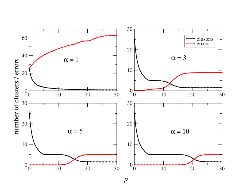
Fig. 4 shows the $N$-dependence of the SCAP results. The parameter $p$ has to be rescaled by $N$ to re-balance the increased number of contributions to the overall similarity in the model’s Hamiltonian. One sees that the initial cluster number for $p=0$ is linear in $N$, but the penalty successfully forces the system to show a collective behavior with macroscopic clusters. The plateau length for different $N$ values is comparable, even if for larger $N$ the decay from the plateau to 1-2 clusters is much more abrupt.

Figure 4: Dependence of the SCAP results for different values of $N$. Curves result from averages over 1000 random samples.

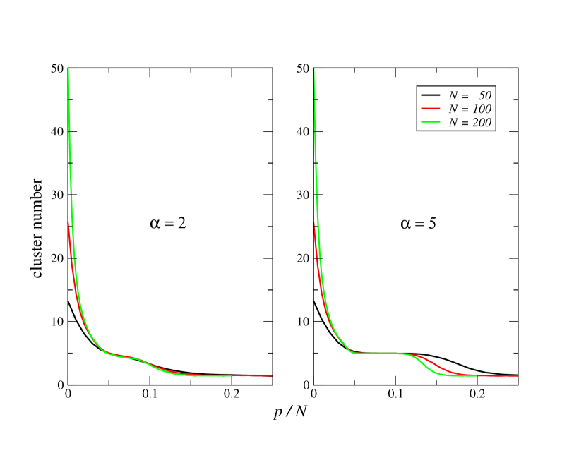
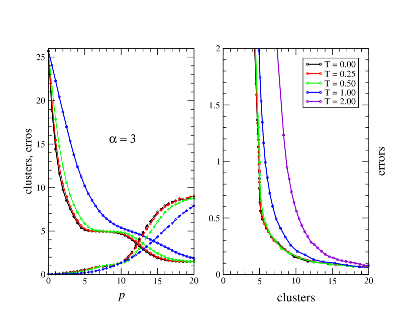
Fig. 5 studies the influence of the formal temperature on SCAP. In some cases finite-temperature SCAP shows more efficient convergence, so it is interesting to see how much information is lost by increasing the formal temperature. The left panel of Fig. 5 represents again the cluster number (resp. error number) as a function of $p$. We see that for very low temperature ($T=0.25$ in the example) results are hardly distinguishable from the zero-temperature results. If we further increase the temperature we observe that the plateau at five clusters becomes less pronounced and shifted to larger $p$. To get rid of this shift, we show in the right panel a parametric plot of the two most interesting quantities: The error number as a function of the cluster number. This plot shows again that the errors start to grow considerably (with decreasing cluster number) as soon as we go below five clusters. For low enough temperatures, the curves practically collapse, so very few of the clustering information is lost. Only for higher temperatures the error number starts to grow already at higher cluster numbers. The pronounced change when we cross the number of clusters is lost. Therefore, as long as the plateau is pronounced in the left panel, also the error number remains almost as low as in zero temperature on the plateau.

Figure 5: Temperature dependence of the SCAP results for $N=100,\,\alpha=3$. The left figure shows the $p$ dependence of the cluster number (full lines) and of the error number (dashed lines). The right figure shows a parametric plot of the numbers of errors vs. clusters. Curves result from averages over 1000 random samples.

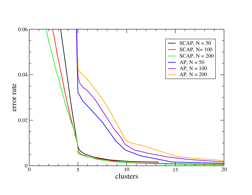
Last but not least, we compare the performance of SCAP to the original AP proposed in FREY . AP shows a slightly different behavior than SCAP. The latter has only one plateau at the correct cluster number, whereas AP shows a long plateau at five clusters, but also less pronounced shoulders at multiples of this number. Both algorithms can be compared directly when plotting the number of errors against the cluster number, see Fig. 6. Note that in principle this test is a bit easier for AP since a part of the data points are self-exemplars, which are not counted as errors. Nevertheless SCAP shows much less errors, in particular also on the plateau of five clusters. The hard constraint in AP forbidding higher order pointing processes is too strong even for a simple data set as the one considered here, simply because the random generation of the similarities makes all points on statistically equivalent, not preferring one as a cluster center. The more flexible structure of SCAP is able to cope with this fact and is therefore results in a more precise clustering. Note that this difference increases with growing size $N$ of the data set: Whereas the error number of SCAP at five clusters slightly decreases with $N$, the corresponding number for AP grows. This is again due to the hard constraint which forces inside a cluster more and more data points to refer to the cluster exemplar.

Figure 6: SCAP vs. AP: The number of errors (divided by $N$) is plotted against the cluster number, for $\alpha=3$ and various values of $N$. Curves result from averages over 1000 samples.

3.2 Hierarchical cluster organization

Figure 7: Artificial data with two-level hierarchical organization. Data (crosses) are organized in clusters (full circles), which themselves are collected in larger clusters (dashed circles). Similarities are drawn from Gaussians as shown in the figure, with $0<\alpha_{0}<\alpha_{1}$.

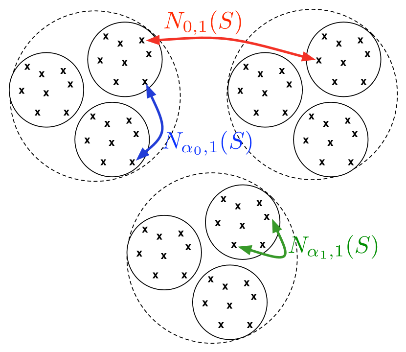
To test if SCAP is also able to detect a hierarchical cluster organization we have slightly modified the generator, as shown in Fig. 7. We divide the set of $N$ data points into $q_{0}$ superclusters, and each of these into $q_{1}$ clusters (in the Fig. $q_{0}=q_{1}=3$). Similarities are drawn independently for each pair of points. If points are in the same cluster, we use a Gaussian $N_{\alpha_{1},1}(S)$ of mean $\alpha_{1}$ and variance 1, if they are in the same supercluster but not in the same cluster, we use $N_{\alpha_{0},1}(S)$, and for all pairs coming from different superclusters we draw similarities from $N_{0,1}(S)$. The means fulfill $0<\alpha_{0}<\alpha_{2}$.

Figure 8: SCAP for a systems with two hierarchical levels of clustering, for $N=180,\ q_{0}=q_{1}=3,\ \alpha_{0}=3,\ \alpha_{1}=6$, averages are performed over 2000 samples. The black line shows the cluster number, two clear plateaus at 9 clusters resp. 3 super-clusters are observed. The red line gives the number of data points selecting an exemplar in a different cluster, the green line even in a different super-cluster. Both quantities are divided by 6 to put them on the same scale as the cluster number.

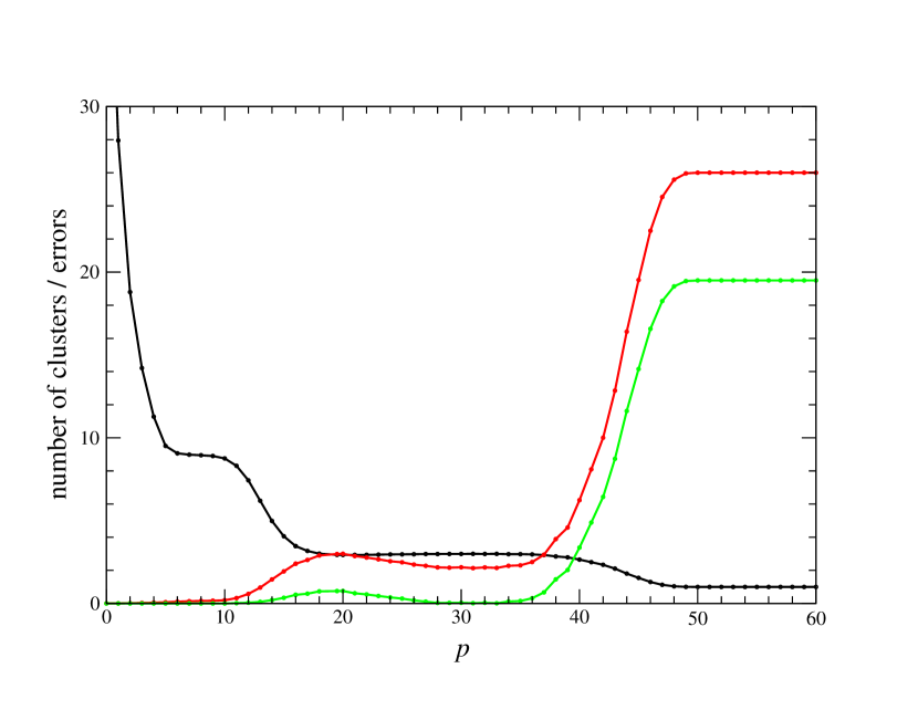
Fig. 8 shows the findings for $N=180,\ q_{0}=q_{1}=3,\ \alpha_{0}=3,\ \alpha_{1}=6$. We clearly see that SCAP is able to uncover both cluster levels, pronounced plateaus appear at 3 and 9 clusters. The plot also shows two different error measures: The number of points which choose an exemplar which is not in the same cluster (red line in the figure), and the number of points choosing even an exemplar in a different supercluster (green line). As long as we have more than 9 clusters, there are very few of both error types (increasing $\alpha_{0}$ further decreases this number). Once we force clusters at the finest level to merge, the first type of error starts to grow. The second grows if we observe some merging of superclusters, i.e. if the cluster number found by SCAP is around or below 3. Note the little bump in the errors at the beginning of the three-cluster plateau: There even some links between different superclusters appear. In fact, in this region the algorithm does not converge in messages in many cases, leading to many errors. In the middle of the plateau, however, convergence is much more stable and error rates are small.

To summarize this section, SCAP is able to infer the cluster structure of artificial data, even if the latter are organized in a hierarchical way. Results are very robust and show less errors than the AP with its hard constraints.

4 Extension to semi-supervised clustering

In case labels are provided for some data points, they can be exploited to enhance the algorithmic performance. We propose the following way: Identically labeled data are collected in macro-nodes, one for each label. Since macro-nodes are labeled, they do not need an exemplar, but they may serve as exemplars for other data. If there are $N$ unlabeled points and $m$ known labels, the exemplar mapping thus gets generalized to ${\bf c}:\{1,...,N\}\mapsto\{1,...,N,N+1,...,N+m\}$ where indexes $N+1,...,N+m$ correspond to macro-nodes. We define the similarity of an arbitrary unlabeled point to a macro-node as the maximum of similarities between the point and all elements of the macro-node . The Hamiltonian now becomes:

$${\cal H}_{2}[{\bf c}]=-\sum_{\mu=1}^{N}S(\mu,c_{\mu})+p_{1}\sum_{\mu=1}^{N}\chi_{\mu}[{\bf c}]+p_{2}\sum_{\nu=N+1}^{N+m}\chi_{\nu}[{\bf c}]$$ (21)

Note that neither the sizes of the training set nor of the macro-nodes appear explicitly. They are implicitly present via the determination of the similarities between data and macro-nodes. In principle, we can choose different values of $p_{1}$ and $p_{2}$, more precisely $p_{1}>p_{2}$, to reduce the cost of choosing macro-nodes as exemplars as compared to normal data points. However, this usually forces data to choose the closest macro-node instead of making a collective choice using the geometrical information contained in the data set. We found $p_{1}=p_{2}=p$ to work best.

Figure 9: Factor graph and message direction: Circles (variable nodes) are unlabeled data points, squares (factor nodes) constraints due to unlabeled (light) and macro-nodes (dark). Similarities act as $(N+m-1)$-dimensional external fields on the unlabeled data points. Messages are exchanged between all connected pairs of data points and constraints.

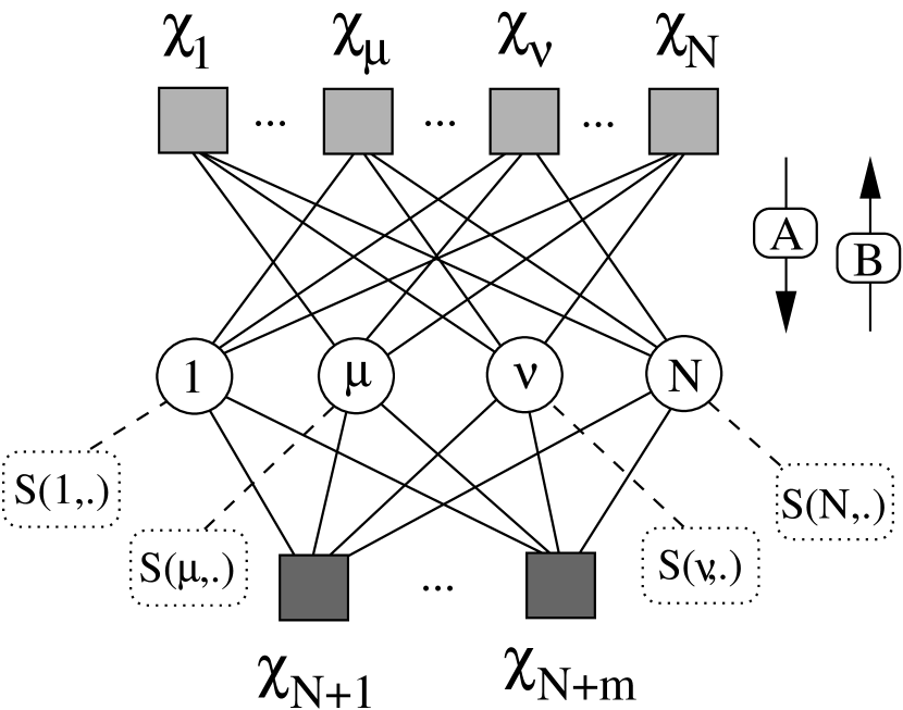
Compared to Fig. 1, the factor graph becomes slightly more complicated. As is shown in Fig. 9, $m$ new factor nodes are added to the graph representing the constraints constituted by the macro-nodes. This modification allows, however, to follow exactly the same route from the Hamiltonian to the final SCAP equations:

$$a_{\mu\to\nu} = {\rm min}[0,\,-p+\sum_{\lambda\neq\mu,\nu}{\rm max}(0,\,r_{\lambda\to\mu})]$$ (22)

$$r_{\nu\to\mu} = S(\nu,\mu)-{\rm max}_{\lambda\neq\mu,\nu}\left[S(\nu,\lambda)+a_{\lambda\to\nu}\right]$$

Remember that $\mu\in\{1,...,N\}$ corresponds to the unlabeled data points, whereas $\nu\in\{1,...,N+m\}$ enumerates the constraints and thus the possible exemplars. At infinite $\beta$, the exemplar choice becomes polarized to one solution (for non-degenerate similarities) and reads

$$c_{\nu}^{\star}={\rm argmax}_{\mu\in\{1,...,N+m\},\mu\neq\nu}\left[S(\nu,\mu)+a_{\mu\to\nu}\right]\ .$$ (23)

Compared to Eqs. (2.3,15) only the number of constraints becomes modified. The introduction of macro-nodes actually allows for a very elegant generalization of SCAP from the unsupervised to the semi-supervised case.

4.1 Artificial data

To test the performance of unsupervised vs. semi-supervised SCAP, we turned first to some artificial cases.

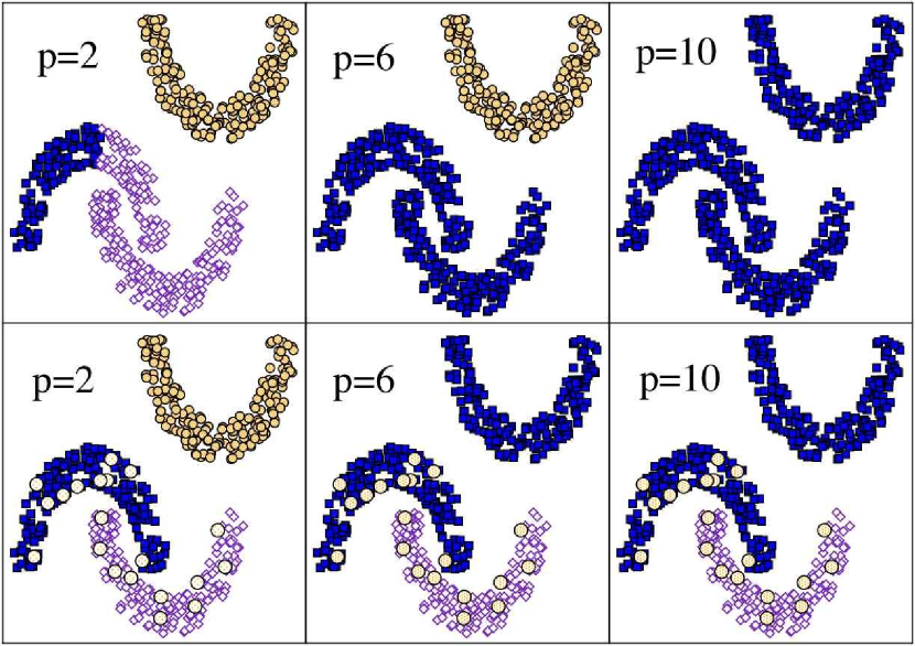
Data set 1: We randomly selected points in two dimensions clustered in a way clearly visible to human eye (Fig. 10). The similarity between data points is measured by the negative Euclidean distance. The clusters are so close that the distance between points on the borders of two clusters is sometimes comparable to the distance between points inside one single cluster. This makes the clustering by unsupervised methods harder. For example, look at Fig. 10, upper row: In this case, the best unsupervised SCAP clustering makes a significant fraction of errors, and does not recognize the two clusters. The best results with unsupervised SCAP are actually obtained when we allow it to divide the data into four clusters.

Figure 10: Upper row: 3 best clusterings seen by unsupervised SCAP. $N=600$, $300$ in each cluster. Lower row: same data set with $t$ trainers (larger circles) for each cluster.

Figure 11: Histogram of the number of errors for 10 000 random choices of $t=5,10,20$ labeled data points. For better visibility, bars are reduced in width and shifted relative to each other for different training-set sizes (bin size 5).

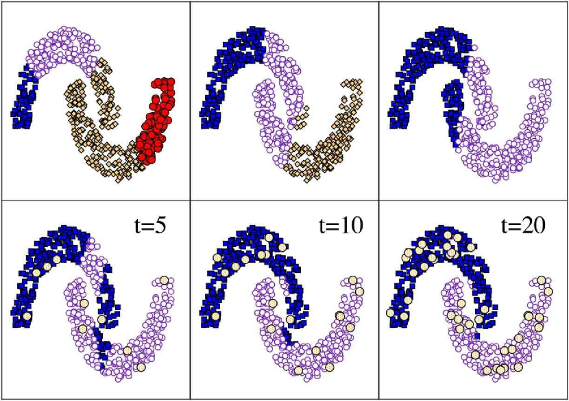
On the other hand semi-supervised SCAP recognizes two clusters very fast. When we introduce some labeled points, we find a significant improvement of the output, cf. Fig. 10, lower row. Already as few as 5 labeled points per cluster increase the performance substantially. Larger training sets lead typically to less errors. In the semi-supervised SCAP, clustering is very stable and does not change when we increase $p$.

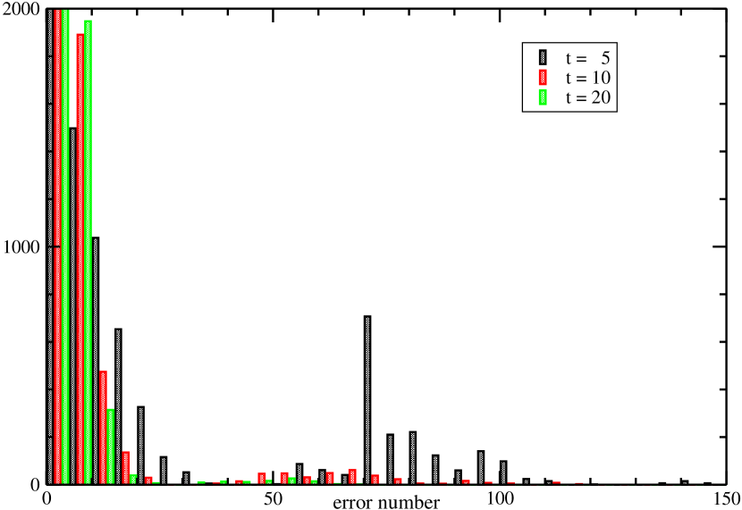
In Fig. 10 we show the clusters for one random choice of labeled set. In general one can argue that the clustering would change with the way the labeled set is distributed inside a cluster. In Fig. 11 we show a histogram for 10000 random selections of the training set, for training set size $t=5,\ 10,\ 20$. We observe that a majority of clusterings found makes only few errors (the peak for less then 5 errors is cut in height for better visibility), but a small number of samples lead to a substantial error number. These samples are found to have labeled exemplars which are concentrated in regions mostly far form the regions where clusters are close, so a relatively large part of these regions is assigned erroneously to the wrong label. The probability of occurrence of such unfavorable situations goes down exponentially with the size of the training data set.

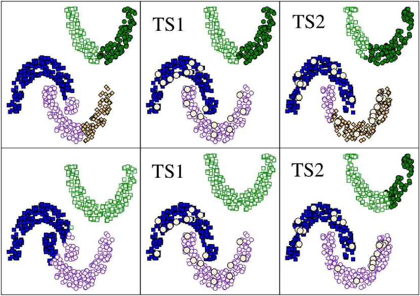
Data set 2: With partial labeling, there are often cases where no information is available on some of the classes. Semi-supervised SCAP is able to deal with this situation because it can output clusters without macro-nodes, i.e. clusters without reference to any of the trainers’ labels. As an example, we add to the artificial data set a third cluster of similar size and shape, without adding any new trainer. As shown in Fig. 12 and 13, the algorithm detects correctly both the labeled and the unlabeled clusters for a wide range of parameters.

Figure 12: Upper row: $N=600$, with 200 data points in each cluster. In all three cases we choose $p=0.5$. In the semi-supervised case $t=10$ each of the lower clusters; $t=0$ for the upper one. The two semi-supervised results are for different training sets (TS1 and TS2). Lower row: same data with $p=1$.

Figure 13: $N=600$, with 200 data points in each cluster. First and second rows contains clustering for unsupervised and semi-supervised learning for $p=2,6,10$ (left to right). Semi-supervised: 10 trainers each for lower clusters, 0 for the upper one. One can see how increasing $p$ leads to an artificial merging of the labeled clusters ($p=6$). However, in the Semi-supervised case a stable region of p arises where the third cluster is well discerned while the labeled ones are still naturally separated.

4.2 Iris data

This is a classic data set used as a bench mark for testing clustering algorithm IRIS . The data consist of measurements of sepal length, sepal width, petal length and petal width, performed for 150 flowers, chosen from three species of the flower Iris. Unsupervised SCAP already works well making only 9 errors. Introducing $t$ trainers per class, the error number further decreases as shown in table 1.

t	3	4-10	15-30	40
errors	7	6	2	1

Table 1: Errors in labeling Iris data, in dependence on the number $t$ of labeled data points.

We also performed semi-supervised clustering where we provided labels for only two out of the three data sets. Depending on the number and distribution of labeled points the algorithm produced 5-9 errors. Semi-supervised SCAP worked better when we provided information on the clusters corresponding to versicolor and virginica species. This is not surprising as these two are known to be closer to each other than to setosa, whose points set is well discerned even in the unsupervised case.

5 Summary and outlook

In this paper, a further simplification of soft-constraint affinity propagation, a message-passing algorithm for data clustering, was proposed. We have presented a detailed derivation, and have discussed time- and memory-efficient implementations. The latter are important in particular for the clustering of huge data sets of more than $10^{4}$ data points, an example would be gene which shall be clustered according to their expression profiles in genome-wide micro-array experiments. Using artificial data we have shown that SCAP can be applied successfully to hierarchical cluster structures, a model parameter (the penalty $p$ for exemplars) allows to tune the clustering to different resolution scales. The algorithm is computationally very efficient since it involves updating ${\cal O}(N^{2})$ messages, and it converges very fast.

SCAP can be extended to semi-supervised clustering in a straightforward way. Semi-supervised SCAP shares the algorithmic simplicity and stability properties of its unsupervised counter part, and can be seen as a natural extension. The algorithm allows to assign labels to previously unlabeled data, or to identify additional classes of unlabeled data. This generalization allows to cluster data even in situations where cluster shapes are involved, and some additional information is needed to distinguish different clusters.

In its present version, SCAP does not yet fully exploit the information contained in the messages, only the maximal excess similarity is used to determine the most probable exemplar. In the case where labels are not exclusive, one can also use the information provided by the second, third etc. best exemplar. This could be interesting in particular in cases, where similarity information is sparse, a popular example being the community search in complex networks.

In a future work we will explore these directions in parallel to a theoretical analysis of the algorithmic performance on artificial data, which will provide a profound understanding of the strength and also the limitations of (semi-supervised) SCAP.

Acknowledgments: We acknowledge useful discussions with Alfredo Braunstein and Andrea Pagnani. The work of S. and M.W. is supported by the EC via the STREP GENNETEC (“Genetic networks: emergence and complexity”).

References

- (1) M. Leone, Sumedha, and M. Weigt, Bioinformatics 23, 2708 (2007).
- (2) A.K. Jain, M.N. Murthy, and P.J. Flynn, ACM Computing Surveys 31, 264 (1999).
- (3) R.O. Duda, P.E. Hart, and D.G. Stork, Pattern Classification, 2nd. ed. (Wiley-Interscience, 2000).
- (4) O. Chapelle, B. Schölkopf, and A. Zien (eds.), Semi-Supervised Learning (MIT Press, Cambridge MA 2006).
- (5) G. Getz, N. Sehntal and E.Domany, Proceedings of “Learning with Partially Classified Training Data” ICML 2005, p.37.
- (6) R.R. Sokal, C.D. Michener, University of Kansas Scientific Bulletin (1958).
- (7) S.C. Johnson, Psychometrika 2, 241 (1967).
- (8) J. McQueen, in Proc. 5th Berkeley Symp. on Math. Stat. and Prob., L. Le Cam, J. Neyman (ed.) (Uni. of California Press 1967).
- (9) M. Blatt, S. Wiseman, and E. Domany, Phys. Rev. Lett. 76,3251 (1996).
- (10) J.S. Yedidia, W.F.Freeman, and Y.Weiss, IEEE Trans. Inform. Theory 47, 1 (2005).
- (11) F.R. Kschischang, B.J. Frey, and H.A. Loeliger, IEEE Trans. Inform. Theory 47, 1 (2001).
- (12) B.J. Frey and D. Dueck, Science 315, 972 (2007).
- (13) M. Mézard and G. Parisi, Eur. Phys. J. B 20, 217 (2001).
- (14) A.K. Hartmann and M. Weigt, Phase Transitions in Combinatorial Optimization Problems (Wiley-VCH, Berlin 2005)
- (15) R.O. Duda, P.E. Hart, Classification and Scene Analysis (Wiley, New York 1973).