Also at: ]LIGO Laboratories, California Institute of Technology, Pasadena, CA 91125
Also at: ]LIGO Laboratories, California Institute of Technology, Pasadena, CA 91125
Bayesian comparison of Post-Newtonian approximations of gravitational wave chirp signals
Abstract
We estimate the probability of detecting a gravitational wave signal from coalescing compact binaries in simulated data from a ground-based interferometer detector of gravitational radiation using Bayesian model selection. The simulated waveform of the chirp signal is assumed to be a spin-less Post-Newtonian (PN) waveform of a given expansion order, while the searching template is assumed to be either of the same Post-Newtonian family as the simulated signal or one level below its Post-Newtonian expansion order. Within the Bayesian framework, and by applying a reversible jump Markov chain Monte Carlo simulation algorithm, we compare PN1.5 vs. PN2.0 and PN3.0 vs. PN3.5 wave forms by deriving the detection probabilities, the statistical uncertainties due to noise as a function of the SNR, and the posterior distributions of the parameters. Our analysis indicates that the detection probabilities are not compromised when simplified models are used for the comparison, while the accuracies in the determination of the parameters characterizing these signals can be significantly worsened, no matter what the considered Post-Newtonian order expansion comparison is.
pacs:
04.80.N, 95.55.Y, and 07.60.LI Introduction
Kilometer-size ground-based interferometric detectors of gravitational radiation have become operational at several laboratories around the world LIGO , VIRGO , GEO , TAMA . From locations in the United States of America, Italy, Germany, and Japan, these instruments have started to search, in the kilohertz frequency band, for gravitational waves emitted by astrophysical sources such as spinning neutron stars, supernovae, and coalescing binary systems.
Among the various sources of gravitational radiation that these instruments will attempt to observe, coalescing binary systems containing neutron stars and/or black holes are expected to be the first to be detected and studied. These signals have a unique signature that enables them to be extracted from wide-band data by digital filtering techniques Helstrom68 . This signature is their accelerating sweep upwards in frequency as the binary orbit decays because of energy loss due to the emission of gravitational radiation. Coalescing binaries have a potential advantage over other sources in signal-to-noise ratio (SNR) by a factor that depends on the square-root of the ratio between the corresponding number of cycles in the wave trains Thorne87 .
The standard technique used for extracting these “chirps” from the noisy data is called Matched Filtering. In the presence of colored noise, represented by a random process , the noise-weighted inner product between the data stream recorded by the detector and the gravitational waveform template is defined as
| (1) |
where the symbol over and denotes their Fourier transform, is the one-sided power spectral density of the noise , , are the limits of the frequency band of interest, and the ∗ represents complex conjugation. From this definition the expression of the SNR can be written in the following form Helstrom68
| (2) |
By analyzing the statistics of the , it is possible to make statements about the presence (or absence) of such a gravitational wave signal in the data. This operation of course needs to be performed over the entire bank of templates over which the SNR statistics is built upon, since a gravitational wave signal is in principle determined by a (finite) set of continuous parameters.
The effectiveness of the matched filtering procedure relies on the assumption of exactly knowing the analytic form of the signal (possibly) present in the data. Recent breakthroughs in numerical relativity P05 ; CLMZ06 ; BCCKM06 have started to provide a complete description of the radiation emitted during the inspiral, merger, and ring-down phases of generic black hole merger scenarios. Although the ability of obtaining numerically all the templates needed in a data analysis search (perhaps hundred of thousands of them) might be practically impossible, in principle we should be able to compare these numerically derived waveforms against various analytic templates obtained under different approximating assumptions. Work in this direction has already started to appear in the literature BCP06 ; BMWCK06 ; PBBCKWPM07 within the so called “frequentist framework”, in which estimates in the reduction in SNRs and inaccuracies of the determination of the parameters characterizing the signal, due to the use of approximated waveforms, have been derived. Depending on the magnitude of these degradations one can decide whether to use these approximated waveforms as templates in a data analysis search.
Since it can be argued that contiguous PN approximations should well characterize the differences between the “true signal” present in the data and the highest-order PN approximation, in this paper we perform such a comparison within the Bayesian framework. An analogous, frequentist analysis has recently been performed by Cutler and Vallisneri CutVallis:2007 for the case of super massive black holes binaries observed by LISA (the Laser Interferometer Space Antenna). Their approach relied on the use of the Fisher-Information matrix, which is known to give good results in the case of large (hundreds to thousands) SNRs. In the case of ground-based interferometers instead, since the expected SNRs will be probably smaller than , a parameter estimation error analysis based on the Fisher-Information matrix would lead to erroneous results Vallis:2007 .
In this paper we will estimate the loss in probability of detection (i.e. loss of evidence of a signal to be present in the data) as a function of the SNR in the following two cases: (i) the true signal present in the data is a spin-less PN3.5 waveform and the search model is represented by a spin-less PN3.0, and (ii) the true signal is a spin-less PN2.0 waveform and the model is a spin-less PN1.5 waveform. We have limited our analysis to these two separate cases in order to cover the region of the PN approximations that have already, or are in the process of, being used in the analysis of the data collected by presently operated ground-based interferometers.
Our approach relies on a Bayesian Markov Chain Monte Carlo (MCMC) technique, as MCMC methods have successfully been applied to a large number of problems involving parameter estimations Gilks:1996 in experimental data sets. In our analysis the chirp signals (the one present in the data and the one used as the model) are characterized by five parameters: the two masses of the system, and , their time to coalescence , the coalescence phase , and their distance from Earth.
Bayesian MCMC methods have already been proven to be capable of estimating the five parameters of a PN2.0 chirp signal embedded into noisy data of a single interferometer when using a PN2.0 based model RoeverMeyerChristensen:2006 , and in a coherent search in the time domain for nine parameters using a PN2.5 model RoeverMeyerChristensen:2007 and a PN3.5 model RoeverMeyerGuidiVicereChristensen:2007 for the phase. However, it has never been shown before how the resulting evidence and probability distributions of the parameters are affected by the usage of different PN models. Here we will estimate the evidence of a signal being buried in noise and, at the same time, derive the probability distribution of its parameters when the gravitational wave form of the model is a simplified version of the signal present in the data. A Bayesian analysis naturally justifies Occam’s Razor Jaynes:2003 ; Loredo:1992 due to the penalization of unreasonably complex models by the integration over the parameter space. The paper is organized as follows. In Section II we provide a brief summary of the Bayesian framework and its implementation in our problem. After deriving the expressions of the likelihood function and the priors for the parameters searched for, in Sec. III we describe the Markov-Chain Monte Carlo sampling technique adopted for calculating the posterior distributions. We then specify in Sec. IV the different simulations we have conducted by introducing the wave forms, noise specifications, and parameter sets. The final results of our simulations are presented in Sec. V, displaying the MCMC based posterior distributions for the parameters and involved models. The estimated posterior probabilities of the models are presented as a function of SNR with the corresponding uncertainties over the noise realizations. We find that the difference in detection probability when using a simplified model rather than the true one is negligibly small in comparison to these uncertainties. The posterior credibility regions of the parameters reveal offsets from the true parameter values that can be much larger than the statistical uncertainty, for both the PN1.5/2.0 and PN3.0/3.5 model comparisons. The PN2.0/2.0 and PN3.5/3.5 comparisons on the other hand, always yield credibility regions that cover the true parameter values. Finally, in Sec. VI we provide our comments and concluding remarks.
II The Bayesian formulation
In this section we will derive the Bayesian full probability model for our problem, which involves the comparison between the two possibilities of having either a signal and noise or just noise in the data. This requires the determination of the likelihoods, the prior distributions for the parameters associated with the models, and the resulting posterior distributions.
II.1 Model definition
Let us suppose we observe a data stream containing the instrumental noise and a chirp signal that we will regard as the “true” signal. Here, is the vector representing all the parameters associated with the signal, and the noise is assumed to be a stationary Gaussian random process of zero mean. In the Fourier domain the observed data can equivalently be written as (where tilde denotes the Fourier transform operation) and we will refer to this expression as model .
In what follows we will assume the “true” signal to be the gravitational wave emitted by a coalescing binary system and represented by a spin-less Post-Newtonian approximation in phase and Newtonian in amplitude for which . Here and are the masses of the rotating objects, is the coalescence time, the absolute distance to the binary system, and the phase of the signal at coalescence.
We will then describe the detection and estimation of the parameters of the “true” signal by relying on a spin-less lower-order Post-Newtonian waveform, . This simpler model will be referred to as model .
The derivation of the detection probability implies a comparison between model and the null-model, which postulates mere noise within the data. This model will bereferred to as model . Note that no parameter enters into this model.
II.2 The likelihood function
Since we have assumed the distribution of the random process associated with the noise of the detector to be Gaussian of zero-mean, it follows that the likelihood function is proportional to the exponential of the integral of the squared and normalized residuals between and signal template over the frequency band of interest . We define the data to be modeled by with its “true” parameter vector . The comparison with the simplified model , results in the following expression for the likelihood function
| (3) |
where is the one-sided power spectral density of the noise.
By substituting into Eq. 3, the likelihood function becomes
| (4) |
In analogy to Eq. 4, under model (with no parameters) the likelihood assumes the following form
| (5) |
For comparison reasons, in the case of using the “true” model the likelihood function becomes
| (6) |
which will then give information about the impairment in detection when using model instead of . Note, that the investigation of this question requires to do the two different model comparisons separately, i.e. vs. and vs. Gregory:2005 .
The next step needed for completing our Bayesian full probability model is the identification of suitable prior distributions for the five parameters characterizing the chirp signal. Our derivation will closely follow that described in RoeverMeyerChristensen:2006 ; RoeverMeyerChristensen:2007 .
II.3 Prior distributions
The derivation of appropriate priors bears significant influence on the evidence of a signal presence within noise, since the prior identifies the size of the parameter space which the evidence is based on.
A detailed description of the derivation of the prior distributions, and in particular for the masses , , and distance , can be found in RoeverMeyerChristensen:2006 ; RoeverMeyerChristensen:2007 . In short, the masses are assumed to be uniformly distributed over a specified range, , and the prior distribution for the distance is chosen to be a cumulative distribution of having systems out to a distance smaller than , , proportional to the cube of the distance, . In order to obtain a proper prior distribution that does not diverge once integrated to infinity, it is down-weighted by including an exponential decaying. This accounts for the Malmquist effect Sandage:2001 and includes the assumption of uniform distribution for the masses. The resulting distribution function can be written as follows RoeverMeyerChristensen:2006
| (7) | |||||
where
| (8) |
and is the so-called “Indicator function”, equal to when and zero elsewhere. The latter term containing the log-amplitude in the sigmoid function of Eq. 7 is the down weighing term mentioned earlier, and it depends on two constants and . These are determined by requiring a smooth transition of a inspiral system being detectable with two specified probabilities at two given distances. In RoeverMeyerChristensen:2006 ; RoeverMeyerChristensen:2007 and are determined by choosing a inspiral system to be detectable with probabilities and out to distances Mpc and Mpc respectively. In our work we will also make such a choice.
Fig. 1 shows the joint prior distribution of the masses , , and marginal distribution of the distance , using Eq. 7. Although initially a uniform distribution is assigned to the masses, the conjunction of distance and masses results in a higher detectability of large masses. The number of possible binary systems increases quadratically with the distance but the down weighing of the prior is significantly seen above Mpc as we allow masses of up to . In RoeverMeyerChristensen:2006 ; RoeverMeyerChristensen:2007 for example, the masses where restricted to and therefore the prior values on the distance were much smaller with a distribution mode at around Mpc.
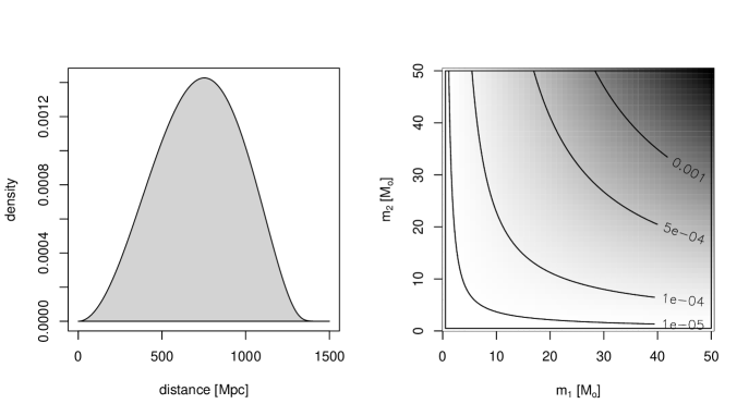
As far as the time to coalescence is concerned, we have assumed it to be uniformly distributed over a time interval of second centered around the value identified by the masses of the binary and the lower frequency cut-off of the detector PDB01 . This search range for the time to coalescence is larger than that used in RoeverMeyerChristensen:2006 because when using the simplified model the posterior peak can be offset from the true value by more than the posterior width.
Finally, we chose the phase of the signal at coalescence, , to be uniformly distributed over the interval , i.e. .
The choice of priors is different when it comes to the analysis of model . Since this model postulates mere noise, there are no parameters entering the likelihood, which is therefore a constant.
The final remaining step in defining the Bayesian procedure is to assign prior probabilities to the models themselves. Since we have no a priori knowledge, the unbiased choice is equal probability for each.
II.4 Posterior distribution
By applying Bayes’ theorem using the likelihoods and priors defined above, we then derive the multidimensional posterior probability distribution for the model and its parameters
| (9) |
where corresponds to the two models . In the same way, it is possible to derive the posterior for the comparison of vs. . A Bayesian analysis naturally justifies Occam’s Razor Jaynes:2003 ; Loredo:1992 due to the penalization of unreasonably complex models by integrating over the parameter space resulting in the preference for a simpler model.
III Bayesian model selection and parameter estimation
There exist various techniques for tackling this multi-dimensional problem. One possible approach is to calculate the so called Bayes factors Kass:1995 ; Han:2001 ; Gregory:2005 , which are the ratios of the global likelihoods of the models that are involved. The Bayesian Information Criterion (BIC) Schwarz:1978 can be used as an approximation to the Bayes factor. However, it is possible to address the problem of sampling from the multidimensional posterior distribution in Eq. 9 by implementing a relatively new procedure, called Reversible Jump MCMC (RJMCMC) technique Green:1995 ; GreenHjortRichardson:2003 , which simultaneously addresses the problems of model selection and parameter estimation. The RJMCMC is combined with traditional fixed dimension MCMC techniques that sample from the parameters of the current model. In the following we will briefly review the MCMC algorithm that we will use in our analysis.
III.1 Metropolis Coupled Markov chain Monte Carlo
In Simulated Tempering Marinari:1992 , the “temperature” becomes a dynamic variable on which a random walk is conducted during the entire sampling process. The joint distribution of temperature and remaining parameters, however, requires the normalization constants of the distributions given the temperature. Other approaches like the Tempered Transition method Neal:1996 or the Metropolis-Coupled chain (a.k.a. parallel tempering algorithm) Geyer:1991 do not need normalization constants. The latter approach has been advocated in the astrophysical literature Gregory:2005 and it has also been implemented in RoeverMeyerChristensen:2007 ; UmstaetterThesis:2006 .
In a Metropolis-Coupled chain Geyer:1991 , sampling is done in parallel from different distributions . The real posterior distribution of interest is denoted by with parameter vector , whereas the distributions of higher orders are chosen in such way that the sampling process is facilitated. Usually, different temperature coefficients are applied Hansmann:1997 that flatten out the posterior modes. During the sampling from the distributions, from time to time, attempts are made to swap the states of a randomly chosen pair of distributions.
The posterior in the present context can be regarded as a canonical distribution
| (10) |
where
| (11) | |||||
with inverse temperatures . For higher values of , the posterior modes are flattened out and the sampling process is eased. A temperature scheme for our Metropolis-Coupled chain uses different values with , where is the temperature of the original posterior distribution. As in UmstaetterThesis:2006 ; RoeverMeyerChristensen:2007 , the prior distribution is purposely not involved in the temperature scheme as the prior information at high temperatures is preserved. Eq. 10 converges to the prior distribution if whereas a temperature scheme, had it been applied to the entire posterior distribution, would merely yield a uniform distribution.
The inverse temperatures are unknown parameters that must be determined prior to each simulation. It is obvious that the highest temperature needs to account for the nature of the likelihood surface. The stronger the signal, the higher the modes and the more likely it becomes for the MCMC sampler to get trapped. The acceptance probability of a proposed jump in a basic Metropolis-Hastings algorithm is determined by the product of the ratios between the proposals, the priors, and the likelihoods Metropolis:1953 ; Hastings:1970 ; Gilks:1996 of the proposed parameter vector and current state parameter vector. For a coarse assessment of the nature of the posterior surface, we can neglect the prior distribution as it is much smoother than the likelihood surface. With symmetric proposals, the likelihood ratio is therefore the key factor in analyzing the depth of the modes in the posterior surface.
Although in the simplified model comparison the parameter estimates can be far off the true parameter values, in the true model comparison the true parameter values are expected to be good estimates of the parameters. This fact can be used for a coarse assessment of the nature of the likelihood surface. Since the log-likelihood of the true model at the true parameter values is , it can be compared to the log-likelihood of the null-model . The probability to overcome a proposed MCMC jump between these two likelihood values determines the convergence of a MCMC sampler. The acceptance probability is therefore related to the difference of the log-likelihoods . We want the hottest temperature to allow jumps within the posterior surface and we want this to happen about every, say, iterations. This number allows occasional jumps at the hottest temperature (smallest inverse temperature) which is therefore chosen to be
| (12) |
We then use an exponential temperature scheme for chains:
| (13) |
For each iteration and each chain, new parameter values are proposed. Of course this is only meaningful when the current state of the chain is not the null-model. If the present state of the sampler is model (or depending on the comparison), independent normal distributions are chosen to propose new jumps. Pilot runs are first used to find appropriate proposal variances. The acceptance probability for a proposed candidate is derived by computing the Metropolis-Hastings ratio Gilks:1996 ; Metropolis:1953 ; Hastings:1970 . The proposed swaps between arbitrary pairs of chains are done in the way described in Geyer:1991 with the temperature scheme highlighted above.
The transdimensional jumps between null-model and model (or ) are conducted by RJMCMC steps Green:1995 . We implemented a death and a birth proposal which either attempts to jump from model (or ) to model or from model to model (or ).
III.2 Reversible Jump Markov chain Monte Carlo
The reversible jump approach requires a random variable with distribution that matches the dimensions of the parameter space across models. In addition, a function is defined that does the dimension matching. In the present case it is a function based on death and birth events. The one-to-one transformation in the ’birth’ transition creates a new signal with parameter vector and has the form . The inverse ’death’ transformation that annihilates the signal, , has form . The Jacobian of both transformations is equal to . The acceptance probability for the creation process is therefore
| (14) |
where is drawn from . The annihilation process is in turn given by
| (15) |
where is the parameter vector of the current existing signal. Since we chose equal prior probabilities for both models, we have .
As one can see in Eq.14, for the creation process, the prior distribution at an existing parameter is found in the enumerator while the proposal distribution at the existing parameter is present in the denominator. On the other hand, in Eq.15, for the annihilation process, the proposal value of a new proposed parameter vector is found in the enumerator while the prior is in the denominator. This means that a larger parameter space, which naturally yields smaller prior values, results in more likely accepted deaths than accepted births. As a consequence, the sampler will prefer sampling from the null-model which means that the evidence of a signal will be smaller if we increase the parameter space. This makes perfect sense as we expect the evidence of a signal to fade if we integrate over a larger parameter space.
The other fact that the proposal distribution enters on opposite sides of the fraction in Eq.14 and Eq.15 reveals the difficulty on the choice of the proposal distribution. In order to understand the effect of the proposal distribution, let us consider the following three scenarios
-
1.
Suppose we do not know the major posterior mode and therefore choose the parameter vector of a new signal to be drawn from a wide spread proposal distribution. We could choose the proposal distribution to be the same as the prior distribution, in which case prior and proposal would cancel out. From the sampling point of view, the samples would account for the prior distribution and the acceptance probability would merely contain the likelihood. However, it would be unlikely to find the narrow mode in the likelihood surface by ineptly poking around in the entire parameter space restricted by the prior. Such a RJMCMC sampler would rarely accept jumps between the models. Only very long runs would give sufficient information about what proportion the sampler naturally stays in which model in order to draw reliable conclusions.
-
2.
Suppose we wrongly assume the posterior mode to be concentrated in some area of the parameter space far away from the actual posterior mode. We would choose the proposal distribution to have the major probability in some wrong area of the parameter space. Naturally the draws from such distribution would privilege proposals in the wrong area of the parameter space but the acceptance probability would repress births and support deaths in the area as the proposal values would be naturally high. The sampler is balanced but mixing would be poor as proposes in the correct area of the parameter space are rare, even though their acceptance would be facilitated. The mixing would be even worse than in the first scenario and even longer runs would be needed to reveal reliable information about how long the sampler naturally stays on average in which model.
-
3.
Suppose we have a vague idea about where the major posterior mode is located and choose our proposal density to be centered around that area. The samples would be drawn preferential in that particular area of parameter space but the ratio of proposal and prior would compensate for that in the acceptance probability. However, the likelihood ratio in this area would have a major impact and the sampler is more likely to jump between the models revealing the proper ratio and model probability in a much shorter sampling period.
We see that the choice of a proper proposal distribution is very important. A good proposal distribution ought to have the major probability mass concentrated around the expected posterior mode but with long tails in order to cover the entire prior. This is achieved by a mixture distribution between a normal distribution with small variance and a uniform distribution that covers the prior range. If we are to compare the null-model and the true model , we are in a lucky position. The mean of the proposal distribution is most likely to be found around the true parameter values and we only need to find a variance in the same order of magnitude as the posterior mode which can be determined by pilot runs.
Things are different when we compare null-model and the simplified model . The posterior mode can not be expected at the true parameter values as the wave form of the simplified model is definitely not best fit at the true parameter values. Just augmenting the variance of a proposal distribution with mean at the true parameter values would result in bad mixing. We therefore need pilot runs at higher signal-to-noise ratio in order to determine the vague center of the posterior mode in the simple model case. The information acquired from such runs serves to determine a suitable proposal distribution.
III.3 Within-model Metropolis-Hastings sampling and re-parameterization
The sampling process of the individual chains when the current state of the Markov chain is in the model that postulates a signal, is done by a common MH step Metropolis:1953 ; Hastings:1970 ; Gilks:1996 . The proposals here is tailored to the expected posterior shape by choosing a very heavy tailed distribution. This was accomplished by mixing a normal distribution with exponentially varying variance UMDVWC:2004 ; MaxEnt:2004 ; UmstaetterThesis:2006 .
The high correlation of the mass parameters , and in the posterior distribution needed to be accounted for by re-expressing them in terms of the following Newtonian and 1.5 PN time to coalescence Chronopoulos:2001
| (16) |
| (17) |
where and . This turned out to work very well as a re-parameterization technique for our sampler.
Since and can be written in terms of and according to the following expressions
| (18) |
| (19) |
where and , it follows that the Jacobian of this transformation is equal to
| (20) |
Since in the original parameter space we defined a joint density for , the new joint prior distribution of , , and is given by
| (21) |
The sampling techniques described in the previous subsections are then used to sample from this new multidimensional parameter space .
IV Description of the simulations
For our simulations we have created data sets from “true” wave forms of three hypothetical binary inspiral systems (BI). We will consider two scenarios where the “true” wave form is either of PN 2.0 or PN 3.5 order. The detection of each scenario is attempted by either a PN 1.5 or a PN 3.0 wave form respectively.
In the first scenario, PN3.0/3.5, “true” model containing a PN3.5 wave form is used for creating the observed data . In the frequency domain a PN3.5 signal has the form Arun:2005 ; CutVallis:2007
| (22) |
where
| (23) |
with
| (24) |
and
| (25) |
and
| (26) |
with coalescence time and coalescence phase , involved masses and , total mass , reduced mass , and chirp mass .
The amplitude is related to the intensity of gravitational wave Chronopoulos:2001 and in the stationary phase approximation, , where is the distance between detector and source. The model is determined by the five parameters . The proportional factor depends on the relative orientation between detector and source, and we will assume it to be constant and equal to since we are more generally interested in the broad assessment of the evidence of a signal.
The signal used for detection is the 3.0 PN approximation, which will serve as the simplified model . The PN3.0 approximation formulated in the frequency domain is given by the following expression
| (27) |
where
| (28) |
In the exact same way the second scenario involving PN1.5/2.0 wave forms is approached where the data are created using a supposedly “true” signal
| (29) |
where
| (30) |
The simplified model uses the lower 1.5 PN expansion
| (31) |
The distance of each binary system is varied in order to obtain different signal-to-noise ratios. The noise realizations are drawn in such a way that they correspond to the approximated expression of the one-sided power spectral density of initial LIGO citeChronopoulos:2001
| (32) |
with being the minimum noise of the detector and Hz the frequency at which the sensitivity of the detector reaches its maximum.
The noise samples are generated directly from the noise spectrum in the following way. Let us assume the noise to be white, Gaussian distributed (i.i.d. standard normal at time ). Its finite Fourier transform is given by
| (33) |
which we can write as
We aim for deriving expected values and variance of the real part and imaginary part of the Fourier transform. Since is normally distributed with zero mean, it follows that also the expectation values and . From this consideration it follows that the variances of the real and imaginary parts of the Fourier transform of the noise are equal to
| (35) | |||||
and in the same way
| (36) |
while the expectation value of the product between the real and imaginary part of the noise is equal to zero. For large it is and . Therefore, the samples of can be generated by sampling and according to a white spectrum of Gaussian noise of variance . These considerations indicate that we can generate the noise samples directly in the Fourier domain by sampling the real and imaginary parts of the noise from two independent random number generators that are Gaussian distributed and have both equal variance ( being the one-sided power spectral density of the noise).
Since the time required to perform a single-signal simulation was several days on the Jet Propulsion Laboratory Dell XEON cluster (running 1024 Intel Pentium 4 Xeon processors), we decided to perform only three simulations for three different binary systems. These were selected to be close to the “corners” of the () region of the mass-space, corresponding respectively to the mass-pairs given in Tab. 1.
| system | |||||||
|---|---|---|---|---|---|---|---|
| B1 | 42.76933s | 0.2 rad | Mpc | ||||
| B2 | 5.26426s | 0.2 rad | Mpc | ||||
| B3 | 0.10778s | 0.2 rad | Mpc |
The reason why we chose binary systems of such particular mass constellations can be seen in the following Fig. 2 where the masses are drawn in the re-parameterized -plane.
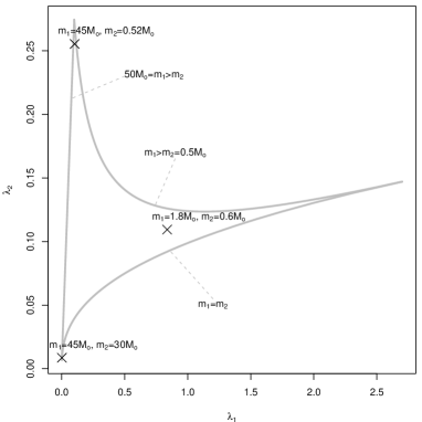
Here, the chirp mass is defined as and the mass function , which is the ratio between the reduced mass and the total mass of the binary system. Fig. 2 shows the three mass constellations close to the three corners of the triangular plane. The bottom left corner corresponds to large masses with low mass ratio, in the top left corner mass constellations are found with large and small masses (large mass ratio). Towards the right corner, the masses become small.
V Results
We created data sets for the three different binary systems given in Tab. 1, and changed their distances in such a way that the resulting SNRs would give a detection probability varying within its extremes. This resulted in varying the SNR within the interval (). For the binary system B1, we simulated 12 different distances of varying step width between and Mpc. We found this step width to be sufficient in order to capture the variability of the calculated detection probability as a function of the SNR. For binary system B2 we similarly took 12 different distances between and Mpc, while for system B3 we considered 16 different distances in the range of Mpc in steps of Mpc. For each of the 40 distances considered we generated 20 different noise realizations, resulting in a total of 800 data sets. Our MCMC sampler was applied four times on each data set for covering the specified model comparisons. This yields a total of simulated Metropolis-Coupled MCMC chains, each of which was stopped after iterations after inspecting that such a number was sufficient for our purpose.
The simulated data were sampled at Hz for a duration of about s, and they were produced by embedding the different signals into noise samples that where generated in the Fourier domain as described in Sec.IV. Since all MCMC runs were conducted after pilot runs at higher SNRs, the burn-in period was kept very short as the proposal distributions were optimized to the target distribution and mixing was very efficient. From the MCMC output we discarded just the first iterations as burn-in, while short-term correlations in the chain were eliminated by “thinning” the remaining terms: every 100 item was kept in the chain.
The integration bandwidth for the likelihood was chosen from Hz up to the frequency of the last stable orbit or Hz, whichever is the smaller. Since the SNR is negligible above Hz, we fixed this to be the upper frequency cut-off. For the B1 system, we derived a frequency of Hz at the last stable orbit which gives an integration limit of Hz for B1. This translates in complex samples that contribute to the posterior distribution. In the case of system B2 instead, the last stable orbit is at Hz, resulting in complex samples involved in the determination of the likelihood function. Finally, for the high mass binary system B3 in our set of systems the last stable orbit is at Hz, implying now only complex samples over which the likelihood is calculated.
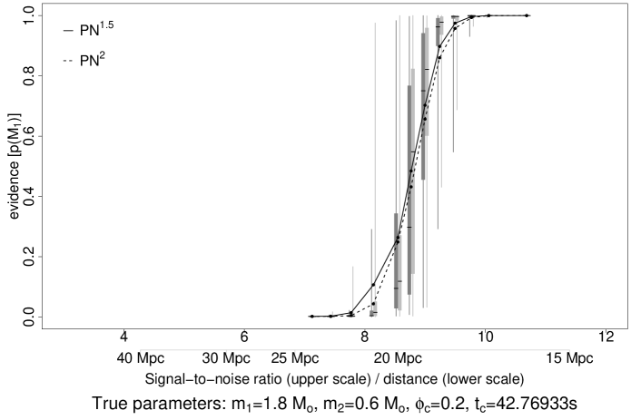
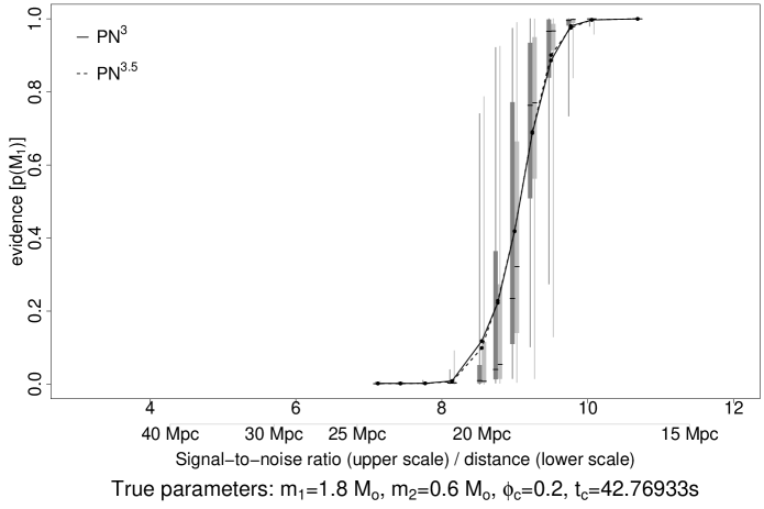
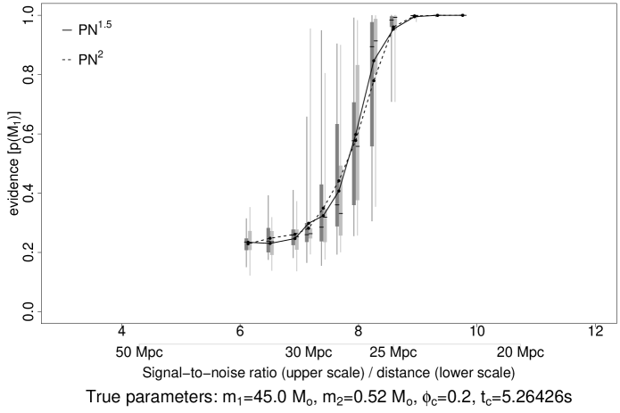
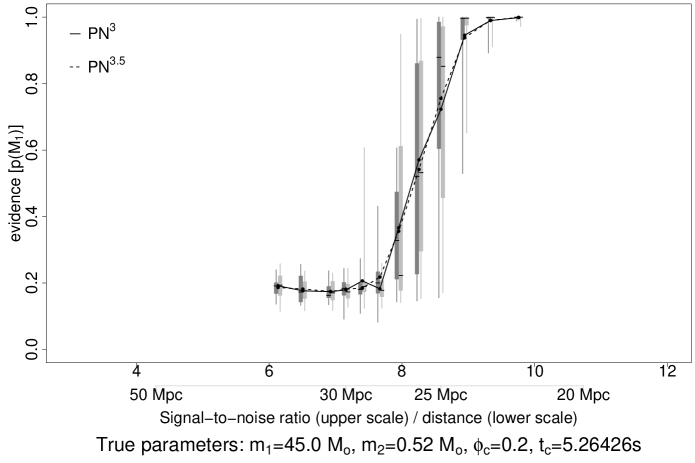
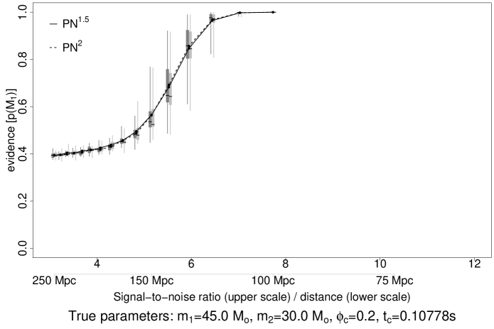
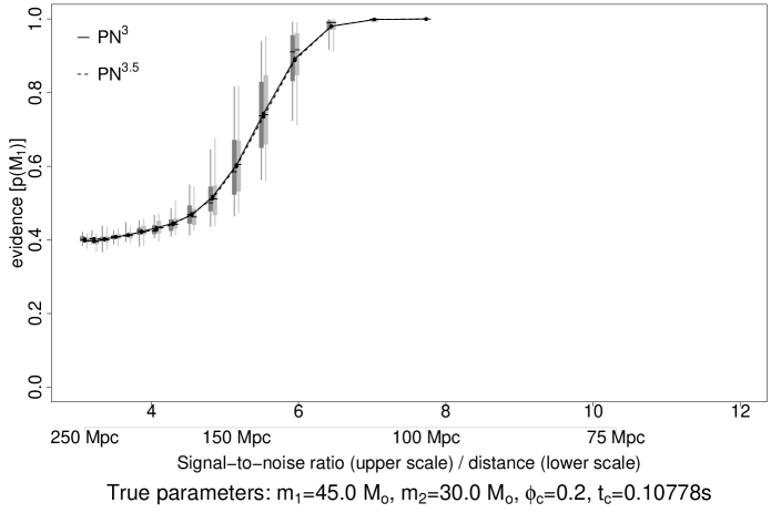
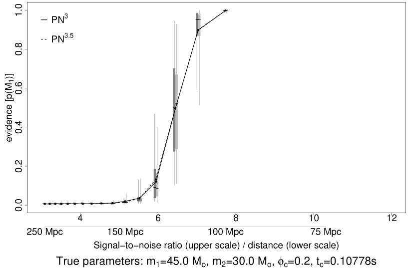
After we conducted the MCMC simulations we derived the posterior detection probabilities for the competing models from the MCMC outputs regarding the three example binary systems, the four different model comparisons, and the different sets of SNRs. For each binary system we computed the posterior probabilities for the considered scenarios and contrasted the probability of detection based on a lower order PN expansion against the one using the true wave form. This is displayed in Figs. 3, 4, 5 respectively.
 |
| (a) |
 |
| (b) |
 |
| (a) |
 |
| (b) |
 |
| (a) |
 |
| (b) |
In order to derive the detection curves we computed the proportions of the states in which the Markov chain recurred to the null model or the model containing a signal. This was done for the entire set of noise realizations for a given SNR. Lines connect the estimates of the posterior detection probabilities resulting in an interpolated function of the SNR. This is a monotonically increasing function of the SNR, reaching asymptotically as the SNR goes to infinity. A common feature to these figures is the uncertainties due to the noise that the signal detection probability shows at a given SNR. In particular, these uncertainties are more pronounced when the gradient of the detection probabilities is at its maximum. Note also that the difference between the detection probabilities associated to the “true model” and the approximated one is much smaller than these uncertainties. The uncertainties are displayed as vertical bars: the 50% quartiles (thick bars), and the outer quartiles (thin lines) associated with the 20 noise realizations. The inner 50% quartiles are divided by a small line which represents the median. It is interesting to see in Fig. 3 that, in some cases, for a given binary system and SNR, detection probabilities as low as or as high as are possible, merely on the effect of the noise realization.
It is worth mentioning that analyses performed within the frequentist framework Chronopoulos:2001 ; Canitrot:2001 ; PBBCKWPM07 and aimed at comparing the detectability of a signal by using a simplified wave form were focused entirely on estimating the resulting loss of SNR. The Bayesian model comparison presented here has the inherent ability to estimate probabilities and their uncertainties due to noise, providing much more insights into this issue.
Another interesting feature shown by the detection probability curves is their asymptotic dependence on the SNR. While the probability of detection always converges to as the SNR goes to infinity, it does not necessarily always goes to zero with the SNR. The reason for this lies in the Bayesian approach in which we assumed equal prior probability for both, the null-model and the model that contains a signal. In the Bayesian context, all probabilities represent a degree of belief. They are based on the prior information and on the information that is given by the data by means of the likelihood. The more data we have, the more new information we obtain from the posterior distribution. The less data we have, the more impact the prior has on the posterior. In an extreme scenario with no data at all, the posterior is equal to the prior. We used this fact to test the correctness of our RJMCMC sampler as it must sample properly from the prior distributions and prior model probabilities when no data are present. The three binary systems considered in this paper each imply different likelihoods. For example B1, with its small masses, has a spectrum that nicely falls into the part of the observable band of the detector where the instrumental noise is at its minimum. On the other hand, the system B3 shows an energy spectrum whose upper frequency cut-off is equal to Hz, with a resulting frequency bins over which the likelihood is calculated.
The diverse data sets are reflected in Figs. 3, 4, 5. For B1 with its involved samples, the detection probability converges to almost zero for low SNRs as the data provide sufficient evidence for the non-existence of a signal even though the prior suggests a probability of . It is in the nature of the Bayesian approach that the scarcer data for B2 and B3 provide less evidence resulting in a posterior detection probability of around and , respectively, when the SNR approaches zero. A different choice for the prior probability on would change the course of the posterior detection curves but with increasing number of data samples and SNR, the likelihood dominates the posterior distribution.
In order to point this up, we created a graph comparable to Fig. 5 (bottom) in which the results of B3 based on the PN3.0/3.5 comparison are shown with a different prior probability of for the null model. The model that contains a signal has consequently a prior probability of .The result is illustrated in Fig. 6.
This plot corresponds to bottom graph of Fig. 5 with the only difference that a more pessimistic prior probability on the null model has been applied. When comparing Fig. 6 to Fig. 5 (bottom), we see that the detection probability is significantly lower at SNR due to the higher prior probability on the null model. However, at an SNR of around , the detection curve jumps up quickly in Fig. 6 and a detection probability of is reached in both figures roughly at an SNR of because the evidence of a signal in the data is overruling the prior probability in both cases.
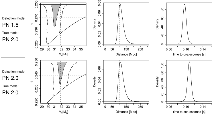
We will now focus on the parameter estimates. We have compiled plots which address the impact of the use of lower PN order wave forms on the bias of posterior distributions of the parameters. Along the lines of Figs. 3, 4, 5, we plot the posterior distributions of the parameters when the posterior detection probability reaches a value of . The posterior distribution of the parameters is hereby an integration over the noise by incorporating all realizations of the MCMC outputs. Each output corresponds to the SNRs at which the detection probabilities in Figs. 3, 4, 5 reach their maximum. We only concentrated on the four parameters , , , as the phase is of no particular physical interest. We displayed the posterior density of the masses as a 2D joint probability density in the form of a contour plot. We computed the two-dimensional 50% and 95% credibility regions.
For the three considered binary systems we generated a total of 36 plots for the distributions of the chirp mass and the mass function , as well as density plots for the distance and the time to coalescence . We have chosen to plot the joint posterior probability of the mass parameters in the -space because they are not as much correlated as in their posterior, which produce hard to visualize posterior densities. Although we could plot the posterior in the space, the joint posterior probability of and is physically more meaningful. We divided the 36 plots into three sets corresponding to B1 (Fig. 7), B2 (Fig. 8), and B3 (Fig. 9).
 |
| (a) |
 |
| (b) |
 |
| (a) |
 |
| (b) |
 |
| (a) |
 |
| (b) |
Figs. 7, 8, 9 display the true parameter values chosen in our simulations (dashed line in the case of and , and intersection of two dashed lines in the plots). From visual inspection we notice that when the model matches the signal present in the data the posteriors cover well the true parameter values. In Fig. 7, however, the joint posterior distribution of the mass parameters are offset from the true values in the PN1.5/2.0 comparison. The PN3.0/3.5 detection, on the other hand, reveals a much smaller offset for this particular signal. However, this is not true in general, as it can be seen for the PN3.0/3.5 comparison shown in Fig. 8. The offsets of the posterior distributions from the true values of the mass parameters are very obvious in both, the PN1.5/2.0 and PN3.0/3.5 comparisons. The posterior is shifted over several of its standard deviation. Very striking is also the error in the time to coalescence for the PN3.0/3.5 comparison in the B2 signal. The mass parameters and and time to coalescence are obviously the parameters subject to biases when using a simplified model. This is physically understandable since these three parameters define the phase of the signal. The posterior distributions of the mass-related parameters shown in Fig. 9 reveal smaller offsets. This is because the spread of the posterior distribution is less pronounced and the bias is therefore smaller compared to the posterior standard deviation. The posterior distribution of time to coalescence, however, is strongly offset from the true parameter value in the PN3.0/3.5 comparison.
The graphical output only serves as a visualization. For an honest comparison, numbers are needed. To this end, in Tab. 2, we show the true values, the 95% posterior credibility interval, the median and the mean of the chirp mass , based on the MCMC outputs. Tab. 3, Tab. 4, and Tab. 5 show the same entries for the parameters , , and , respectively. The right-most column of the tables compares whether the true values of the binary systems fall into the corresponding 95% posterior credibility intervals.
| simulation | 95% credibility | posterior | posterior | true value falls | |
|---|---|---|---|---|---|
| identification | true value | interval (CI) | mean | median | into 95% CI |
| B1: PN1.5/2.0 | |||||
| B1: PN2.0/2.0 | |||||
| B1: PN3.0/3.5 | |||||
| B1: PN3.5/3.5 | |||||
| B2: PN1.5/2.0 | |||||
| B2: PN2.0/2.0 | |||||
| B2: PN3.0/3.5 | |||||
| B2: PN3.5/3.5 | |||||
| B3: PN1.5/2.0 | |||||
| B3: PN2.0/2.0 | |||||
| B3: PN3.0/3.5 | |||||
| B3: PN3.5/3.5 |
The results seen in these tables show that the mass function, , and the time to coalescence, , are the parameters that are most biased when estimated with a simplified model. Note, first of all, that in all cases, the true values fall into the 95% credibility intervals when the estimation is based on the true model. For the distance and the chirp mass the 95% credibility intervals cover the true values in all comparisons. However, when applying a simplified model, the 95% credibility interval of the mass function does not cover the true value in three cases: {B1:PN1.5/2.0, B2:PN1.5/2.0, and B2:PN3.0/3.5)}. In the case of the time to coalescence , we find instead four cases: {B2:PN1.5/2.0,B2:PN3.0/3.5,B3:PN1.5/2.0,B3:PN3.0/3.5}. Combining these cases, we have a total of 5 out of the 6 simple model comparisons (PN1.5/2.0 and PN3.0/3.5) that fail to retrieve all their parameters within the 95% credibility region. The only simple model comparison that yields 95% credibility intervals that overlap all the true parameter values is B1: PN1.5/2.0, although this is only marginal.
In summary, we see that the bias in the estimated parameters based on a simpler model is larger than the statistical uncertainty. However, we should note that the SNR we have been considering corresponds to the value at which the posterior detection probability just reaches the value of one. Since the statistical error is a monotonically decreasing function of the SNR while the bias is not, we conclude that the difference between statistical and systematic error increases for larger SNRs.
These results reveal that parameter estimates based on simplified models are not very reliable, since the systematic error is higher than the uncertainty of the posterior distribution. Furthermore, the use of higher order post Newtonian wave forms does not abate this problem, as it has been shown in Fig. 8.
VI Conclusion
We have shown that, within the Bayesian framework, the probability of detection is not impeded by using a simplified model for detecting wave forms of higher PN order in the low-SNR regime. The Bayesian approach provides the means to gain insight into the variation of the detection probability over different noise realizations. We have shown that the difference between the posterior detection probabilities corresponding to the true and the simplified model is very small as compared to its variance over different noise realizations. We have further shown that the systematic error in the Bayesian estimates, on the other hand, can be larger than the statistical uncertainties. This is also in agreement with results obtained within the frequentist approach, discussed in the literature by others Chronopoulos:2001 ; Canitrot:2001 ; PBBCKWPM07 . However, it is based on finding the best fit of the involved wave forms while in our Bayesian framework an integration is performed over the entire posterior distribution which implies detection and estimation simultaneously. We can therefore analyze the posterior distributions, conditioned on the model that involves a signal which provides us with credible estimates in the low-SNR regime.
We find that the estimates of and based on simplified models need to be taken with caution in both the PN1.5/2.0 and in the PN3.0/3.5 case as the offset is unpredictable. The only parameter that is accurately recovered throughout our simulations is the distance which is clear as it only appears in the amplitude term and is not affecting the phase evolution of the signal. The chirp mass could also be retrieved within the 95% credibility intervals but yet shows a visible offset. With increasing SNR, however, the statistical error becomes smaller while the systematical offset remains constant. Given these findings we conclude that post Newtonian approximations, regardless of order, can be precarious for detecting “true” gravitational wave forms.
VII Acknowledgments
This research was performed at the Jet Propulsion Laboratory, California Institute of Technology, under contract with the National Aeronautics and Space Administration. The supercomputers used in this investigation were provided by funding from JPL Office of the Chief Information Officer. This work was supported by the NASA Postdoctoral program Fellowship appointment conducted at JPL (R.U.), and by the research task 05-BEFS05-0014 (M.T.).
References
- [1] The LIGO project home page is at http://www.ligo.caltech.edu.
- [2] The virgo project home page is at http://www.virgo.infn.it/.
- [3] The geo-600 project home page is at http://www.geo600.uni-hannover.de/.
- [4] The tama project home page is at http://tamago.mtk.nao.ac.jp/.
- [5] C.W. Helström, editor. Statistical Theory of Signal Detection. Pergamon Press, London, 1968.
- [6] K.S. Thorne. Gravitational radiation. In Three Hundred Years of Gravitation, pages 330–458. Cambridge University Press, 1987. S.W. Hawking, and W. Israele, eds.
- [7] F. Pretorius. Evolution of binary black-hole spacetimes. Physical Review Letters, 95:121101, 2005.
- [8] M. Campanelli, C.O. Lousto, P. Marronetti, and Y. Zlochower. Accurate evolutions of orbiting black-hole binaries without excision. Physical Review Letters, 96:111102, 2006.
- [9] J.G. Baker, J. Centrella, D. Choi, M. Koppitz, and J. van Meter. Gravitational-wave extraction from an inspiraling configuration of merging black holes. Physical Review Letters, 96:111102, 2006.
- [10] A. Buonanno, G. B. Cook, and F. Pretorius. Inspiral, merger, and ring-down of equal-mass black-hole binaries. Physical Review D, 75:124018, 2006.
- [11] J.G. Baker, J.R. van Meter, S.T. McWilliams, J. Centrella, and B.J. Kelly. Consistency of post-newtonian waveforms with numerical relativity. Classical and Quantum Gravity, pages arXiv:gr–qc/0612024v1, 2006.
- [12] Y. Pan, A. Buonanno, J.G. Baker, J. Centrella, B.J. Kelly, S.T. McWilliams, F. Pretorius, and J.R. van Meter. A data-analysis driven comparison of analytic and numerical coalescing binary waveforms: nonspinning case. Classical and Quantum Gravity, page arXiv:0704.1964v1, 2006.
- [13] C. Cutler and M. Vallisneri. Lisa detections of massive black hole inspirals: parameter extraction errors due to inaccurate template waveforms. Classical and Quantum Gravity, page arXiv:0707.2982, 2007.
- [14] M. Vallisneri. Use and abuse of the fisher information matrix in the assessment of gravitational-wave parameter-estimation prospects. Classical and Quantum Gravity, pages arXiv:gr–qc/0703086, 2007.
- [15] W. R. Gilks, S. Richardson, and P. J. Spiegelhalter, D. J. Green, editors. Markov chain Monte Carlo in practice. Chapman and Hall, London, 1996.
- [16] C. Röver, R. Meyer, and N. Christensen. Bayesian inference on compact binary inspiral gravitational radiation signals in interferometric data. Classical and Quantum Gravity, 23(15):4895–4906, August 2006.
- [17] C. Röver, R. Meyer, and N. Christensen. Coherent Bayesian inference on compact binary inspirals using a network of interferometric gravitational wave detectors. Physical Review D, 75(6):062004, March 2007.
- [18] C. Röver, R. Meyer, G. M. Guidi, A. Viceré, and N. Christensen. Coherent Bayesian analysis of inspiral signals. Classical and Quantum Gravity, 24(19):S607–S615, October 2007.
- [19] E. T. Jaynes. Probability Theory: The Logic of Science. Cambridge University Press, 2003.
- [20] T. J. Loredo. Statistical challanges in modern astronomy, chapter The promise of Bayesian inference for astrophysics, pages 275–297. Springer-Verlag, New York, 1992.
- [21] P. C. Gregory, editor. Bayesian Logical Data Analysis for the Physical Sciences. Cambridge University Press, 2005.
- [22] A. Sandage. Encyclopedia of Astronomy and Astrophysics. Institute of Physics Publishing, Bristol, 2001.
- [23] A. Pai, S. Dhurandhar, and S. Bose. Data-analysis strategy for detecting gravitational-wave signals from inspiraling compact binaries with a network of laser-interferometric detectors. Physical Review D, 64:042004, 2001.
- [24] R. E. Kass and A. E. Raftery. Bayes factors. Journal of the American Statistical Association, 90(430):773–795, 1995.
- [25] C. Han and B. P. Carlin. Markov chain Monte Carlo methods for computing Bayes factors: A comparative review. Journal of the American Statistical Association, 96(455):1122–1132, 2001.
- [26] G. Schwarz. Estimating the dimension of a model. The Annals of Statistics, 6(2):461–464, 1978.
- [27] P. J. Green. Reversible jump Markov chain Monte Carlo computation and Bayesian model determination. Biometrika, 82(4):711–732, 1995.
- [28] P. J. Green, N. L. Hjort, and S. Richardson, editors. Highly Structured Stochastic Systems. Oxford University Press, 2003.
- [29] E. Marinari and G. Parisi. Simulated tempering: A new Monte Carlo scheme. Europhysics Letters, 19:451–454, 1992.
- [30] R. M. Neal. Sampling from multimodal distributions using tempered transitions. Statistics and Computing, 6:353–366, 1996.
- [31] C. J. Geyer. Markov chain Monte Carlo maximum likelihood. In E. M. Keramidas, editor, Computing science and statistics: Proceedings of the 23rd Symposium on the Interface, pages 156–163. Interface Foundation, Fairfax Station, VA, 1991.
- [32] R. Umstaetter. Bayesian Strategies for Gravitational Radiation Data Analysis. PhD thesis, University of Auckland, 2006.
- [33] U. H. E. Hansmann. Parallel tempering algorithm for conformational studies of biological molecules. Chemical Physics Letters, 281:140–150, 1997.
- [34] N. Metropolis, A. W. Rosenbluth, M. N. Rosenbluth, A. H. Teller, and E. Teller. Equation of state calculations by fast computing machines. Journal of Chemical Physics, 21(6):1087–1092, 1953.
- [35] W. K. Hastings. Monte Carlo sampling methods using Markov chains and their applications. Biometrika, 57:97–109, 1970.
- [36] R. Umstätter, R. Meyer, R.J. Dupuis, J. Veitch, G. Woan, and N. Christensen. Estimating the parameters of gravitational waves from neutron stars using an adaptive MCMC method. Classical and Quantum Gravity, 21:S1655–S1665, 2004.
- [37] R. Umstätter, R. Meyer, R.J. Dupuis, J. Veitch, G. Woan, and N. Christensen. Detecting gravitational radation from neutron stars using a six-parameter adaptive MCMC method. In AIP Conference Proceedings - Bayesian inference and Maximum Entropy Methods in Science and Engineering: 24th, volume 735, pages 336–343. American Institute of Physics, 2004. International Workshop on Bayesian Inference and Maximum Entropy Methods in Science and Engineering.
- [38] A.E. Chronopoulos and T.A. Apostolatos. Less accurate but more efficient family of search templates for detection of gravitational waves from inspiraling compact binaries. Physical Review D, 64:042003, 2001.
- [39] K. G. Arun, B. R. Iyer, B. S. Sathyaprakash, and P. A. Sundararajan. Parameter estimation of inspiralling compact binaries using 3.5 post-newtonian gravitational wave phasing: The nonspinning case. Physical Review D, 71:084008, 2005.
- [40] P. Canitrot. Systematic errors for matched filtering of gravitational waves from inspiraling compact binaries. Physical Review D, page 082005, 2001.