First excitations in two- and three-dimensional random-field Ising systems
Abstract
We present results on the first excited states for the random-field Ising model. These are based on an exact algorithm, with which we study the excitation energies and the excitation sizes for two- and three-dimensional random-field Ising systems with a Gaussian distribution of the random fields. Our algorithm is based on an approach of Frontera and Vives which, in some cases, does not yield the true first excited states. Using the corrected algorithm, we find that the order-disorder phase transition for three dimensions is visible via crossings of the excitations-energy curves for different system sizes, while in two-dimensions these crossings converge to zero disorder. Furthermore, we obtain in three dimensions a fractal dimension of the excitations cluster of . We also provide analytical droplet arguments to understand the behavior of the excitation energies for small and large disorder as well as close to the critical point.
pacs:
75.10.Nr, 75.40.Mg, 02.60.Pn, ,
1 Introduction
Many disordered systems are characterized by an extremely rough energy landscape [1, 2, 3]. This leads to the existence of configurations that are quite different from ground-state configurations but have an energy very close to the ground-state energy. The behavior of such systems differs considerably from the behavior of ordered systems and has attracted the attention of many physicists during the last decades. The most prominent example of a magnetic system with quenched disorder exhibiting many valleys in the energy landscape is the spin-glass model [4].
Another basic model from statistical physics that exhibits quenched disorder is the random-field Ising model (RFIM). In the RFIM, the sensitivity to the actual configuration of the disorder and the roughness of the energy landscape are not as strong as in spin glasses but nevertheless present and important to understand the behavior [5].
A RFIM sample consists of Ising spins on a -dimensional regular hypercubic lattice with lateral length in each dimension. Neighbouring spins interact ferromagnetically with strength . In addition, on each site a random magnetic field acts on spin . The are quenched random variables chosen according to some probability distribution. One common choice is a Gaussian normal distribution of zero mean and standard deviation . With a Gaussian disorder, the ground state and the FES are nondegenerate.
The Hamiltonian of the RFIM is
| (1) |
The current state of knowledge on the Gaussian RFIM can be sketched as follows: No ordered phase can persist in the infinite system for , the lower critical dimension is [6]. For , there is a continous phase transition at a critical field between an ordered ferromagnetic phase and a disordered paramagnetic phase [7]. It is possible to analyse the phase transition at zero temperature since the random fields are a relevant perturbation as shown by Fishman and Aharony [8].
Compared to other disordered models such as spin glasses, the RFIM has the practical advantage that in any dimension the problem of finding the ground state can be solved with fast graph-theory based algorithms. This means that the running time increases only like a low-order polynomial in . This has led to numerous studies of the ground state landscape of the RFIM, e.g. [7, 9, 10]. The system sizes that can be analyzed this way are considerably larger than those that can be equilibrated via Monte-Carlo techniques at small temperatures [11, 12].
Using these approaches one is not restricted to study only ground states. Even better, it is also possible to study the properties of the RFIM at very low but nonzero temperatures with suitably modified ground-state techniques. To do this, the ground state must be perturbed in some way to gain low energy states. Various attempts have been made in this direction, among them Refs. [5, 7].
In this study, we investigate first excited states (FESs) in the RFIM and their differences to ground states. In particular we present in Sec. 2 an algorithm to obtain exact FESs, in contrast to a previous attempt [13], where some FESs were missed. In Sec. 3, we show first that indeed a considerable fraction of true FESs was missed in Ref. [13]. Next we apply our algorithm to study FESs both in the ordered and disordered phase. In particular, we investigate the scaling behavior of the excitation energy and the fractal properties of the FESs. These findings are finally contrasted with arguments based on extreme-value considerations and on the droplet theory for the excitations in a hierarchical landscape. Finally, we finish with conclusions.
2 Algorithm
A fast ground-state algorithm for the RFIM was first suggested in Ref. [14] and is explained in detail in Ref. [15]. The main idea is to transform the RFIM to a network consisting of a directed, weighted graph . is the set of nodes and being the set of edges. are edge labels denoting capacities. There are two distinguished nodes and called the source and the sink. All other nodes are called inner nodes. In , a -cut is defined as a partition of into two disjoint sets and with and . We call and the two sides of the cut. To each , a capacity
| (2) |
is assigned. Note, this means that only edges with the “right” direction contribute to . We will also use an equivalent description of a cut by a vector () with if for and else.
The problem of finding the ground state of the RFIM can be reduced to the problem of finding the cut with the smallest capacity among all possible cuts in such a network. This problem can be solved by determining the maximum flow of the network, as proven by Ford and Fulkerson [16]. As already mentioned, the ground state is nondegenerate, hence is also unique for the model with Gaussian distribution of the random fields.
We will now describe the algorithm of finding the first excited state as developed by Frontera and Vives (FV), adopting most of their terminology. By means of an example, we show why there are cases in which this algorithm fails to find the FES. The necessary adjustments are subsequently explained.
Let be a network corresponding to a RFIM sample. Its minimum cut can be calculated with a maximum-flow algorithm. We say an edge is contained in , if and . We denote the set of edges that are contained in as and write . The set of nodes that are on either side of any edge is called , i.e. .
The set of all possible cuts (corresponding to all possible spin configurations) of is . Any edge divides into two disjoint subsets, the set of cuts that contain and the set that do not.
Next, a second network is defined that includes a perturbation of strength . The difference between and is that the capacity of one edge of the minimum cut is increased by an amount , so that
| (3) |
Each cut of is also well defined in , but its capacity has increased if is contained in . For the remaining cuts of that do not contain , the capacity does not change, i.e.
| (4) |
Since we chose , is the cut with
the minimum capacity in for both and
(the capacity of all cuts of is
increased by in ). The minimum cut of
the complementary set is called
. For and all other cuts of this set,
the capacity is the same in both networks.
It follows that depending
on , there are two possibilities for the minimum cut of
:
| (5) |
If is chosen large enough (e.g. , the maximum flow in the ground state), the minimum cut of is always .
Let be the cut with the second smallest capacity in , corresponding to the first excited state. This cut must differ from the minimum cut by at least one edge. Frontera and Vives claim that because of this, “there exists (at least) one edge of so that is in ”. We will show below that this assumption is not always true.
To understand the algorithm of Frontera and Vives, we assume for a moment that the assumption is true. Then, in order to find the capacity of the second minimum cut, one would have to choose a suitably large . After that, is determined for all networks depending on the edges contained in the minimum cut . From all the resulting cuts, the one with the minimum capacity in the original network is accepted and called .
| (6) |
However, the FES has not necessarily been found yet, since the algorithm still has a problem: It assumes that the minimum cut necessarily includes an edge that the second minimum cut does not include. This is wrong, since there is also the possibility that all edges of the minimum cut are still contained in the second minimum cut which differs from the old one in that it additionally contains another edge.
This can be illustrated by looking at Fig. 1, an example network where the GS cut is drawn in. When the capacity of the edge connecting with node is enlarged by a sufficiently large amount , the flow through the new network is limited by the edges to the sink. Therefore, in the resulting cut that is shown in the figure, all inner nodes have changed their side of the cut, and the capacity of is . is not identical with the true second minimum cut that is depicted in Fig. 2 and has a capacity , so that .
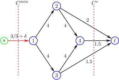
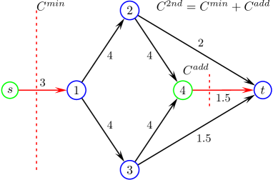
We change the algorithm by leaving the original algorithm untouched (obtaining an intermediate cut after the first step) and introducing a second step. In this step, we go through all nodes except those belonging to . For each of these nodes , we consecutively check if it is favorable to assign to the other side of the cut (in the vector notation of a cut, set if and vice versa). This would result in a new cut for which . As a result, additional edges contribute to the capacity of . We denote their contribution with so that . Note that performing this test for a node belonging to would result also in removing some edges from the cut, hence this is already taken care of by the FV algorithm.
If there are nodes where , the FES is given by the minimum cut among the nodes , if no such node exists, the FES is .
Note that there can never be a negative contribution to since with this would mean to remove an edge that was included in in the GS (while adding other edges at the same time). But in this case the removed edge would have been already considered in the first step.
For the extension of the FV algorithm, it is sufficient to look at single
spin flips, i.e. at moving exactly one node from one side of the cut
to the other. We explain this for a node with , the
other case can be treated analogously. The change
for affects the
capacity of the new cut in the following way:
There are possibly nodes
and . In this case
an amount of is added to as soon as is set to .
Since there are no predecessor nodes
with =1,
hence incoming edges into do not have to be considered for
the calculation of , due to (2).
It might seem plausible that there exist situations where, instead of adding the capacities to , also node (and possibly more nodes) should be moved to the other side of the cut. In fact, some of these situations would lead to a smaller . However, in such a situation it would lead to an even smaller (remember that we are only interested in the second smallest cut) to invert only node instead of inverting both node and node . This is due to the fact that with our method, there can never be a negative contribution to .
The pseudo code for the full algorithm for calculating the FES is shown in Fig. 3.
| algorithm First Excited State |
| Transform the RFIM to a network |
| Calculate of that corresponds to the ground state |
| with |
| for each edge Frontera-Vives algorithm |
| minimum cut of |
| if then |
| end if |
| end for |
| for all nodes extension to obtain true FES |
| if then |
| for all nodes with |
| end for |
| else if then |
| for all nodes with |
| end for |
| end if |
| if |
| with node inverted |
| end if |
| end for |
| return and |
| end |
Finally, we discuss the running time of the algorithm. The running time of the FV algorithm scales like [13] when the running time of the minimum cut has scales as . The additional part introduced here is linear in and therefore does not increase the full running time of the algorithm in a noticeable way.
3 Results
We calculated first excited states of samples at different random field strengths and different system sizes up to in (resp. in ). For the largest three-dimensional system size , samples were calculated at each .
A comparison of the states generated with the Frontera-Vives algorithm with those generated using the complete algorithm that is described above, shows that the differences are noticeable though not drastic. For small systems in with spins at , the FV algorithm does not find the true FES in of the cases. With growing system size, this percentage decreases. In two-dimensional samples (systems of this size were mainly investigated in [13]), the percentage is and in three-dimensional systems of , of the excitations generated by the FV algorithm are incorrect - both in the ferromagnetic and paramagnetic region. In the transition region between the two phases, the error rate is considerably smaller since a large number of first excited states consist of more than one spin and are therefore spotted correctly by the FV algorithm.
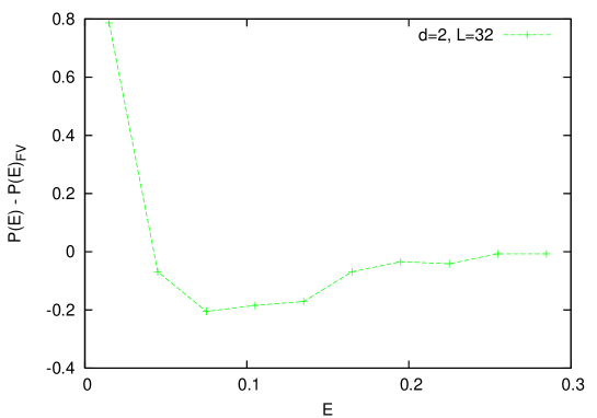
Since the FV algorithm creates states with a higher excitation energy, the difference is also visible in the distributions of the excitation energy. The difference is positive for small and negative for larger , as shown in Fig. 4.
In our analysis of the properties of the FESs, the main quantities of interest are the energy difference to the GS and the size of the excitation cluster, given by the number of spins that change their orientation in the FES. By plotting the disorder-averaged excitation energy against for various , we see that for large , the becomes independent of , i.e. . The value of the plateau scales like .
For that reason, we rather plot instead of vs. . The resulting curve for is shown in the main part of Fig. 5, the corresponding curve for is plotted in the inset.
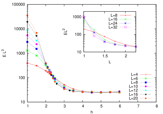
For , the curves of all system sizes coincide as expected. Slightly above the phase transition, the rescaled energy grows with decreasing . For larger systems, the slope is larger. An interesting point is that in the different curves intersect in a narrow region that is close to . This behavior can only be seen in three dimensions. In there is no single intersection point and the intersections approache with increasing , reflecting the absence of a phase transition in two-dimensions [6]. Hence, it seems to be possible to locate the phase transition from the scaling behavior of the excitation energy. We are not aware of previous similar findings. In the next section, we will show by simple droplet arguments, that indeed the energy close to should display a behavior. Nevertheless, we are not able to give a full explanation of this behavior around , which seems to originate from corrections to scaling.
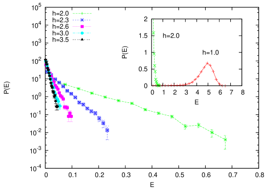
The energy distributions are shown in Fig. 6 for fixed . Close to and beyond the distribution seems to be exponential, as we also find using the simple droplet arguments in the next section. In the inset, the extremely ferromagnetic case is depicted. is peaked at a large in completely ferromagnetic samples, corresponding to flipping spins against the orientations of all neighbors. For a detailed discussion, see again below. Small excitations cannot occur, there is an energy gap between the GS and the FES.
The average size (i.e. the number of flipped spins) of the FES is shown in Fig. 7. Global flips were not taken into account for this plot.
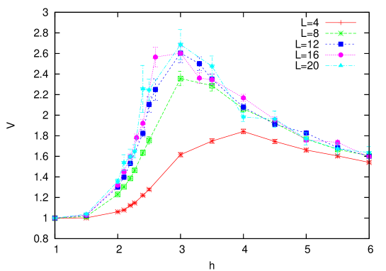
In the ferromagnetic phase, is equal to one. For , it also decreases slowly towards . Thus, in both cases, the FES behaves as expected above. In between, there is a maximum with a size that seems to grow with . The value of where the maximum is located depends on . It shifts towards with growing system size. This is due to the fact that finite systems are most “critical” at a field that approaches when . Since for first excited states, we are restricted to rather small system sizes and the statistical errors are still significant, it remains unclear if the maximum really moves to for larger systems.
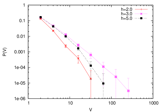
The probability distribution of the excitation volumes is shown in the double logarithmic plot of Fig. 8. Both in very paramagnetic () and ferromagnetic () systems, declines in a fast way. At near the peak of Fig. 7, the decay is not so fast and resembles at least for small a power law. However, to verify that approaches a power law at for large systems, much larger systems would be necessary.
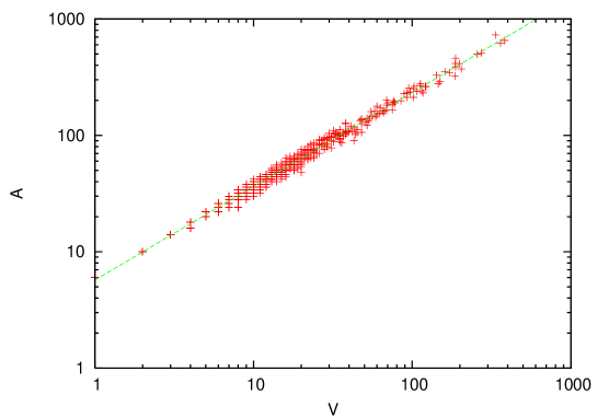
We also analyzed the shape of the excited clusters. The surface of a cluster is given by the number of bonds that connect a spin of the cluster with another spin which is not part of the cluster. By plotting against the volume of the clusters, we gain information on the fractal dimension of the cluster. Since we found that the clusters are compact (, not shown) it follows that . From Fig. 9 (, ) it follows that , leading to which can be compared with an earlier result of Middleton and Fisher [7] obtained for domain-walls.
4 Extreme-value and droplet arguments for the minimal excitations
Now, we try to understand the behavior of the distribution of the droplet energy and the average via analytical arguments for the extreme cases and as well as in the region where the droplet theory holds, hence close to .
The relation for large can be explained by a simple extreme-value argument, which e.g. has also been used to explain the low-temperature behavior of spin glasses [17]. If , the system behaves paramagnetically. Hence, FESs will be essentially single-spin flip excitations which is indeed true for the simulation data, as we have seen above. In this case, the spin with the smallest total local field will flip for the FES. Due to the paramagnetic state, there will be many spins with the same number of “up” neighbors and “down” neighbors. Hence, the total local field will be the same as the quenched local field . The energy of the FES will be given by the smallest absolute value among these spins.111There might be also spins with the number of “up” spins not equal to the number of “down” spins, but with the total local field close to zero. Nevertheless, since the Gaussian is peaked at zero, those will much less frequently comprise the FES compared to the spins discussed here. Thus, the excitation energy is given by the minimum of absolute values of Gaussian random numbers. For simplicity, we assume :
| (7) |
The distribution function of the sample minimum of numbers from a distribution with for is
| (8) |
If is continuous and has a finite weight at the origin (which is true for a Gaussian distribution), one can approximate by for large and gets
with , having the mean
agrees with the numerical simulation data of the mean energy and the predicted exponential decay of occurs indeed in the numerical data and can be seen in Fig. 6
The limit of strongly ferromagnetic systems can also be understood. In
the ferromagnetic phase, there are two possibilities for the FES:
In
smaller samples, the entire system can flip. This
happens if the excess of the random fields is even
smaller than the minimum bond energy that has to be invested for
flipping a single spin. If all spins flip, the bond contribution of
the total energy stays invariant and the random field contribution
changes its sign, so that the
excitation energy is . However, this type of excitation
cannot persist in large systems, since becomes soon
larger than the energy of a second type of excitations, the local
reversal of a single spin. This energy decreases for larger systems:
If the system is fully magnetized, all spins are pointing in the same direction. We discuss the case that all spins are pointing “down”, the reverse case is similar. Hence, we have for all spins. Then, from the spins where the local field is positive, the spin with the maximum local field will have the smallest local field, i.e. will be chosen to be flipped for the FES. Since six bonds of strength from to its neighbors are no longer satisfied, the excitation energy is in three dimensions. So we seek for the sample maximum in the ferromagnetic case.
The sample maximum of values drawn from a distribution has the distribution
| (9) |
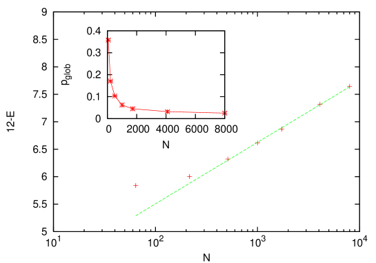
We calculated the integrals numerically and determined the expected value for sample sizes up to . It was found that grows in a logarithmic way with . Therefore we expect that will also grow in a logarithmic way in systems that are large enough that global spin flips are negligible.
The comparison with the numerical data of the FES deep in the ferromagnetic phase at is shown in Fig. 10. In the inset, the probability of a global flip is plotted versus . This probability decreases quickly, and for , global flips occur already in less than of the samples. In the main part, is plotted versus . grows in a logarithmic way as expected, and deviations occur only for the smallest samples where global spin flips are still frequent.
The droplet argument for the minimal excitation, which should be valid close to , starts with the assumption that the contributions from various scales are independent. Further, one takes their (scale-dependent) energy density to scale as , where is the energy fluctuation exponent [18]. The value in 3D is currently found to be by ground-state simulations to be [7]. On scale , for small energies , one will have thus the cumulative excitation energy distribution .
The smallest excitation energy in the whole system is then given by the minimum over all the scales. At each scale, the system splits into independent subvolumes. The minimum excitation energy from a scale has the cumulative distribution
| (10) |
where . This comes simply from the argument that the complement of indicates that all the subvolumes have a smallest excitation of higher energy than . Similar ways of reasoning have been used in other disordered systems [19].
The minimal energy (cumulative) distribution over all the scales can be constructed similarly. The droplet enery is smaller or equal to if the converse is not true: that all the scales would have a minimum higher than that. Thus we obtain
| (11) |
The product is now taken over logarithmic scales, so that .
The product can be converted by standard tricks to a sum and then to an integral, or computed numerically from
| (12) |
where one notes that the argument of the exponential has a prefactor coming from the .
The resulting definite integral, using (), is of the type and does not appear to have a simple closed form solution. Integrating, with fixed over produces for the probability Figure 11. We see that in analogy to the numerical findings for paramagnetic 3d systems the minimum excitation energy distribution is exponential. Here, in is just chosen at random to a small constant. In reality, when the droplet argument is valid it should depend on dimensionality and . Figure 12 shows for a range of values the resulting average droplet energy . In agreement with the most clear-cut numerical data in 3d, the scaling is volumelike ().


5 Summary and discussion
In this paper, we have first presented an algorithm that calculates first excited states in the random-field Ising model. We showed that a former algorithm developed by Frontera and Vives does not find the true first excited states in all cases but and therefore needs to be extended. When comparing the correct algorithm with the Frontera-Vies algorithm, we find that the difference in quantities such as the excitation energy is measurable albeit not drastic for larger systems.
The excitations consist of connected clusters of spins which are reversed with respect to the ground state. In our simulations we study mainly the three-dimensional RFIM, but we also present some results for two dimensions for comparison. Interestingly, there is an intersection of the curves for different system sizes at a point very close to the phase transition point . This behavior cannot be found in the two-dimensional case and seems to reflect the existence of a phase transition.
The volume distribution exhibits a peak close to that becomes sharper with growing system size. However, the size distribution at a fixed near the peak is relatively broad so that statistical errors are large. The fractal dimension of the clusters was determined to be .
Using analytical arguments, we were able to understand the behavior of the average excitation energy in the extreme cases and . To further investigate the origins of the observed energies and their scaling, we have used a droplet argument to derive the energy distribution of the minimal excitations. This line of reasoning is similar to a few others found in the literature (see again e.g. [19], but we are not aware of any where the whole distribution would have been written down. The result reproduces well some features of the numerics, as a volume-like scaling of and the exponential character of the . Hence, the such calculated behavior at follows our numerical observations. Additional corrections to scaling close to seem to be responsible for the observed behavior of the crossing of the curves.
For future work, it would be interesting to look at other types of low excitations with ground states that do not necessarily produce the FES but still a low energy state. States of this kind can be generated much more efficiently, leading to larger systems that can be simulated. Another possibility would be to analyze excitations in higher dimensional systems (see [20] [21] for results in ). However, different approaches from the FES algorithm would have to be used for that since we were already restricted to relatively small system sizes in three dimensions.
6 Acknowledgments
The authors have received financial support from the VolkswagenStiftung (Germany) within the program “Nachwuchsgruppen an Universitäten”, and from the European Community via the DYGLAGEMEM program. MJA would like to acknowledge the support of the Center of Excellence program of the Academy of Finland.
References
- [1] A. P. Young, editor. Spin glasses and Random Fields. World Scientific, Singapore, 1989.
- [2] K. H. Fischer, J. Hertz. Spin Glasses. Cambridge University Press, Cambridge, 1991.
- [3] M. Mézard, G. Parisi, M. Virasoro. Spin Glass theory and beyond. World Scientific, Singapore, 1986.
- [4] K. Binder, A. P. Young. Spin glasses: Experimental facts, theoretical concepts, and open questions. Rev. Mod. Phys., 58:801 – 976, 1986.
- [5] M. Alava, H. Rieger. Chaos in the random field Ising model. Phys. Rev. E, 58:4284, 1998.
- [6] J. Bricmont, A. Kupiainen. Phase transition in the 3d random field Ising model. Communications in Mathematical Physics, 116:539–572, 1988.
- [7] A. A. Middleton, D. S. Fisher. Three-dimensional random-field Ising magnet: Interfaces, scaling and the nature of states. Phys. Rev. B, 65:13411, 2001.
- [8] S. Fishman, A. Aharony. Random field effects in disordered anisotropic antiferromagnets. J. Phys. C, 12:L729–733, 1979.
- [9] A. K. Hartmann, U. Nowak. Universality in three dimensional random-field ground states. Eur. Phys. J. B, 7:105, 1999.
- [10] A. K. Hartmann, A. P. Young. Large-scale low energy excitations in the two-dimensional Ising spin glass. Phys. Rev. B, 66:094419, 2002.
- [11] M. E. J. Newman, G. T. Barkema. Monte Carlo study of the random-field Ising model. Phys. Rev. E, 53:393, 1996.
- [12] H. Rieger. Critical behavior of the three-dimensional random-field Ising model: Two-exponent scaling and discontinuous transition. Phys. Rev. B, 52:6659, 1995.
- [13] C. Frontera, E. Vives. An algorithm for finding the first excited state in the random-field Ising model. Journal of Computational Physics, 169:219–226, 2001.
- [14] J. P. Picard and H. D. Ratliff. Minimum cuts and related problems. Networks, 4:357, 1975.
- [15] A. K. Hartmann, H. Rieger. Optimization Algorithms in Physics. Wiley-VCH, Berlin, 2001.
- [16] L. R. Ford, D. R. Fulkerson. Maximal flow through a network. Can. J. Math., 8:399–404, 1956.
- [17] A. J. Bray, M. A. Moore. Lower critical dimension of Ising spin glasses: a numerical study. J. Phys. C, 17:L463–L468, 1984.
- [18] D. Fisher, A. Huse. Nonequilibrium dynamics of spin glasses. Phys. Rev. B, 38:373–385, 1988.
- [19] A. A. Middleton. Energetics and geometry of excitations in random systems. Phys. Rev. B, 63:060202, 2001.
- [20] A. K. Hartmann. Ground-state clusters of two-, three-, and four-dimensional +/-J Ising spin glasses. Phys. Rev. E, 63:016106, 2000.
- [21] A. A. Middleton. Scaling, domains, and states in the four-dimensional random field Ising magnet. cond-mat/0208182, 2002.