Multipartite entanglement measure for all discrete systems

Beatrix C. Hiesmayr and Marcus Huber
Faculty of Physics, University of Vienna, Boltzmanngasse 5, A-1090 Vienna, Austria
Abstract

Via a multidimensional complementarity relation we derive a novel operational entanglement measure for any discrete quantum system, i.e. for any multidimensional and multipartite system. This new measure admits a separation into different classes of entanglement obtained by using a flip operator 222โ€“, 333โ€“,โ€ฆ, n๐‘›nโ€“times, defining a m๐‘šmโ€“flip concurrence. For mixed states bounds on this m๐‘šmโ€“flip concurrence can be obtained. Moreover, the information content of a n๐‘›nโ€“partite multidimensional system admits a simple and intuitive interpretation. Explicitly, the three qubits system is analyzed and e.g. the physical difference in entanglement of the W๐‘ŠWโ€“state, the Gโ€‹Hโ€‹Z๐บ๐ป๐‘GHZโ€“state or a biโ€“separable state is revealed.

pacs:
03.67.Mn

I Introduction

For many quantum mechanical applications entanglement is the basic ingredient. Mathematically entanglement is well defined. However, no simple operational criterion to detect entanglement versus separability is known. Especially with multipartite entanglement, which is subject to recent research (Ref.ย theory3 ; theory4 ; theory5 ; theory6 ; theory7 ; theory8 ; Meyer ; Boixo ), there are still many open questions regarding its properties. Moreover, it is known that there exist different โ€œkindsโ€ of entanglement, see e.g. Ref.ย Horodeckibig . It is therefore highly desirable to first find an operational measure of entanglement and secondly it should provide a good classification of the different kinds of entanglement as this is the physical property which is explored by various applications such as e.g. quantum cryptography or quantum communication, see also Ref.ย theory1 ; experiment1 ; experiment2 .

In this paper we provide both by defining a novel and very intuitive entanglement measure which is additive for pure states and has the advantage to separate entanglement into 222โ€“, 333โ€“,โ€ฆ, n๐‘›nโ€“flip entanglement and for certain cases even into bipartite, tripartite,โ€ฆn๐‘›nโ€“partite entanglement. It works for any dimension and any number of particles.

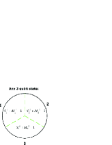
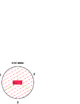
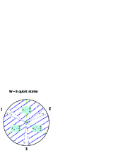
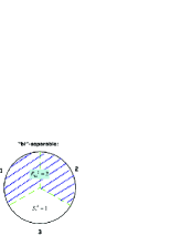
Explicitly, we show for three qubit systems how this novel measure admits the separation of entanglement into genuine bipartite and tripartite entanglement. And moreover how its substructure is revealed, i.e. the entanglement property of each qubit with all others, see also Fig.ย 1.

(a)Refer to caption (b)Refer to caption (c)Refer to caption (d)Refer to caption

Figure 1: Here the information content of three qubits states, 3=โˆ‘s=13(Ss2+Ms2)=โˆ‘s=13Ss2+E12+E23+E13+E1233superscriptsubscript๐‘ 13subscriptsuperscript๐‘†2๐‘ superscriptsubscript๐‘€๐‘ 2superscriptsubscript๐‘ 13subscriptsuperscript๐‘†2๐‘ subscript๐ธ12subscript๐ธ23subscript๐ธ13subscript๐ธ1233=\sum_{s=1}^{3}(S^{2}_{s}+M_{s}^{2})=\sum_{s=1}^{3}S^{2}_{s}+E_{12}+E_{23}+E_{13}+E_{123}, is visualized. In (a) Bohrโ€™s complementarity relation for each qubit is drawn. (b) visualizes the GHZโ€“state, 12โ€‹{|000โŸฉ+|111โŸฉ}12ket000ket111\frac{1}{\sqrt{2}}\{|000\rangle+|111\rangle\}, which is a genuine tripartite state, the bipartite and single properties are zero. In (c) the Wโ€“state, 13โ€‹{|001โŸฉ+|010โŸฉ+|100โŸฉ}13ket001ket010ket100\frac{1}{\sqrt{3}}\{|001\rangle+|010\rangle+|100\rangle\}, is visualized, the single properties are nonzero as well as the bipartite entanglement. In (d) the โ€œbiโ€โ€“separable state, Eq.ย (22), is drawn, which shows as desired only bipartite entanglement though the 333โ€“flip concurrence is nonzero. Therefore, as desired, the particle 333 is independent of particle 111 and 222.

For that we start by proposing the following separation of the information content in a n๐‘›nโ€“partite quantum state of arbitrary dimension ฯ๐œŒ\rho:

Iโ€‹(ฯ)+Rโ€‹(ฯ)โŸsingle property+Eโ€‹(ฯ)โŸentanglement=nsubscriptโŸ๐ผ๐œŒ๐‘…๐œŒsingle propertysubscriptโŸ๐ธ๐œŒentanglement๐‘›\displaystyle\underbrace{I(\rho)+R(\rho)}_{\textrm{single property}}+\underbrace{E(\rho)}_{\textrm{entanglement}}=n (1)

where

Iโ€‹(ฯ)๐ผ๐œŒ\displaystyle I(\rho) :=assign\displaystyle:= โˆ‘s=1n๐’ฎs2โ€‹(ฯ)โŸsingle property of subsystem ssuperscriptsubscript๐‘ 1๐‘›subscriptโŸsuperscriptsubscript๐’ฎ๐‘ 2๐œŒsingle property of subsystem s\displaystyle\sum_{s=1}^{n}\underbrace{{\cal S}_{s}^{2}(\rho)}_{\textrm{single property of subsystem s}} (2)

We will show that for certain cases:

  • โ€ข

    Iโ€‹(ฯ)๐ผ๐œŒI(\rho) contains all locally obtainable information,

  • โ€ข

    Eโ€‹(ฯ)๐ธ๐œŒE(\rho) contains all information encoded in entanglement,

  • โ€ข

    Rโ€‹(ฯ)๐‘…๐œŒR(\rho) is the complementing missing information, due to a classical lack of knowledge about the quantum state.

Moreover, we show how the total amount of entanglement can be separated into m-flip concurrences:

Eโ€‹(ฯ)๐ธ๐œŒ\displaystyle E(\rho) :=assign\displaystyle:= C(2)2โ€‹(ฯ)โŸtwo flip concurrence+C(3)2โ€‹(ฯ)โŸthree flip concurrence+(โ€ฆ)subscriptโŸsuperscriptsubscriptC22๐œŒtwo flip concurrencelimit-fromsubscriptโŸsuperscriptsubscriptC32๐œŒthree flip concurrenceโ€ฆ\displaystyle\underbrace{\textbf{C}_{(2)}^{2}(\rho)}_{\textrm{two flip concurrence}}+\underbrace{\textbf{C}_{(3)}^{2}(\rho)}_{\textrm{three flip concurrence}}+\;\quad(\dots) (3)
+ย C(n)2โ€‹(ฯ)โŸn-flip concurrence.subscriptโŸsuperscriptsubscriptย C๐‘›2๐œŒn-flip concurrence\displaystyle+\underbrace{\textbf{ C}_{(n)}^{2}(\rho)}_{\textrm{n-flip concurrence}}\,.

Furthermore we show that with help of the m-flip concurrence we can, at least for three qubits and possibly for even more complex systems, indeed find a quantity interpretable as:

Eโ€‹(ฯ)๐ธ๐œŒ\displaystyle E(\rho) =\displaystyle= E(2)โ€‹(ฯ)โŸbipartite entanglement+E(3)โ€‹(ฯ)โŸtripartite entanglementsubscriptโŸsubscript๐ธ2๐œŒbipartite entanglementsubscriptโŸsubscript๐ธ3๐œŒtripartite entanglement\displaystyle\underbrace{E_{(2)}(\rho)}_{\textrm{bipartite entanglement}}+\underbrace{E_{(3)}(\rho)}_{\textrm{tripartite entanglement}} (4)

with the substructure:

E(2)โ€‹(ฯ)โŸโŸsubscript๐ธ2๐œŒ\displaystyle\underbrace{E_{(2)}(\rho)} =\displaystyle= E(12)โ€‹(ฯ)+E(23)โ€‹(ฯ)+E(13)โ€‹(ฯ)subscript๐ธ12๐œŒsubscript๐ธ23๐œŒsubscript๐ธ13๐œŒ\displaystyle E_{(12)}(\rho)+E_{(23)}(\rho)+E_{(13)}(\rho) (5)

We proceed in defining or deriving step by step the involved quantities and discuss their physical content.

II The single property ๐’ฎssubscript๐’ฎ๐‘ {\cal S}_{s} and Bohrโ€™s complementary relation:

Bohrโ€™s complementary relation was first discussed to understand the double slit experiment, its information theoretic content can be formulated by the following formula GreenbergerYasin ; Englert :

๐’ฎ2โ€‹(ฯ):=๐’ซ2โ€‹(ฯ)+๐’žcoh2โ€‹(ฯ)โ‰ค1,assignsuperscript๐’ฎ2๐œŒsuperscript๐’ซ2๐œŒsuperscriptsubscript๐’žcoh2๐œŒ1\displaystyle{\cal S}^{2}(\rho):={\cal P}^{2}(\rho)+{\cal C}_{\textrm{coh}}^{2}(\rho)\leq 1\;, (6)

where for all pure states the equality sign is valid. ๐’žcโ€‹oโ€‹hsubscript๐’ž๐‘๐‘œโ„Ž{\cal C}_{coh} is the coherence or in the case of the double slit scenario the fringe visibility which quantifies the sharpness or contrast of the interference pattern (โ€œthe waveโ€“like propertyโ€). Whereas ๐’ซ๐’ซ{\cal P} denotes the path predictability, i.e., the a priori knowledge one can have on the path taken by the interfering system (โ€œthe particleโ€“like propertyโ€). In double slit experiment it is simply defined by ๐’ซ=|PIโˆ’PIโ€‹I|๐’ซsubscript๐‘ƒ๐ผsubscript๐‘ƒ๐ผ๐ผ{\cal P}\;=\;|P_{I}-P_{II}|, where PIsubscript๐‘ƒ๐ผP_{I} and PIโ€‹Isubscript๐‘ƒ๐ผ๐ผP_{II} are the probabilities for taking each path (PI+PIโ€‹I=1)P_{I}+P_{II}=1).

As has been shown this complementary relation is useful to understand several interfering two state system as e.g. particleโ€“antiparticle mixing systemsย HH1 ; SBGH3 or Mott scattering experiments of identical nuclei SBGH3 or even specific thermodynamical quantum system HV .

One can make Bohrโ€™s complementary relation always exact by adding the quantity (dimensionality d๐‘‘d, here 222)

M2โ€‹(ฯ)=ddโˆ’1โ€‹(1โˆ’Tโ€‹rโ€‹(ฯ2))superscript๐‘€2๐œŒ๐‘‘๐‘‘11๐‘‡๐‘Ÿsuperscript๐œŒ2\displaystyle M^{2}(\rho)=\frac{d}{d-1}\left(1-\,Tr(\rho^{2})\right) (7)

to the single particle property ๐’ฎ๐’ฎ{\cal S}

๐’ฎ2โ€‹(ฯ)+M2โ€‹(ฯ)=1superscript๐’ฎ2๐œŒsuperscript๐‘€2๐œŒ1\displaystyle{\cal S}^{2}(\rho)+M^{2}(\rho)=1 (8)

for all states (pure: Mโ€‹(ฯ)=0๐‘€๐œŒ0M(\rho)=0). Mโ€‹(ฯ)๐‘€๐œŒM(\rho) measures the mixedness or linear entropy which equals in this case the uncertainty of individual particles under investigation, clearly a โ€œclassicalโ€ uncertainty.

The complementarity principle seems to be an intrinsic property of all discrete quantum systems. So even considering various dynamics that a quantum system can be exposed to HH1 , the two dimensional complementarity relation still holds true. The next logical step is trying to generalize this relation to for a qudit system.

III Bohrโ€™s complementary relation for d๐‘‘dโ€“dimensional systems

: For a qudit system or a multiโ€“slit system the definition of predictability is not straightforward. One approach has recently been introduced in Ref.ย Janos2 ; Bergou , however, we introduce a similar approach which makes a generalization to multipartite systems possible. To do that we will first introduce the following useful quantity

Pi,jsubscript๐‘ƒ๐‘–๐‘—\displaystyle P_{i,j} :=assign\displaystyle:= Tโ€‹rโ€‹(ฯโ€‹|iโŸฉโ€‹โŸจj|)๐‘‡๐‘Ÿ๐œŒket๐‘–bra๐‘—\displaystyle Tr\left(\rho\,|i\rangle\langle j|\right) (9)

and propose the generalized predictability for a qudit state ฯ๐œŒ\rho

Pgโ€‹(ฯ):=assignsubscript๐‘ƒ๐‘”๐œŒabsent\displaystyle P_{g}(\rho):=
dโˆ’1dโ€‹โˆ‘ฯ€|P0,0โˆ’P1,1+P2,2+(โ€ฆ)+Pdโˆ’1,dโˆ’1dโˆ’1|2๐‘‘1๐‘‘subscript๐œ‹superscriptsubscript๐‘ƒ00subscript๐‘ƒ11subscript๐‘ƒ22โ€ฆsubscript๐‘ƒ๐‘‘1๐‘‘1๐‘‘12\displaystyle\sqrt{\frac{d-1}{d}\sum_{\pi}\left|P_{0,0}-\frac{P_{1,1}+P_{2,2}+(...)+P_{d-1,d-1}}{d-1}\right|^{2}}
=\displaystyle= ddโˆ’1โ€‹โˆ‘i|Pi,iโˆ’1d|2=ddโˆ’1โ€‹โˆ‘iPi,i2โˆ’1dโˆ’1,๐‘‘๐‘‘1subscript๐‘–superscriptsubscript๐‘ƒ๐‘–๐‘–1๐‘‘2๐‘‘๐‘‘1subscript๐‘–superscriptsubscript๐‘ƒ๐‘–๐‘–21๐‘‘1\displaystyle\sqrt{\frac{d}{d-1}\sum_{i}|P_{i,i}-\frac{1}{d}|^{2}}=\sqrt{\frac{d}{d-1}\sum_{i}P_{i,i}^{2}-\frac{1}{d-1}}\;,

where โˆ‘ฯ€subscript๐œ‹\sum_{\pi} denotes the sum over all possible permutations of Pi,jsubscript๐‘ƒ๐‘–๐‘—P_{i,j}. The first line admits for a multi-slit scenario the following simple interpretation: it is the difference of the probability that the particle transverses the slit, e.g. P0,0subscript๐‘ƒ00P_{0,0}, minus the probabilities that the particle takes the way through all the other slits weighted by dโˆ’1๐‘‘1d-1, summed over all slits. For d=2๐‘‘2d=2 it is clearly equivalent to the prior definition of predictability, it ranges from zero to one and is equal to one if one has hundred per cent information about a possible measurement outcome and it is equal to zero if one does not have any information about which degree of freedom would most likely to be measured. Thus is meets all of our conceptual requirements.

Of course it is only one of many ways to describe multi-level predictability, but one that meets all of our conceptual requirements. A different one was introduced in Ref.ย Janos2 .

The coherence is easier to define, it is more straightforward. We can just take the sum over all two dimensional coherences:

Ccโ€‹oโ€‹h,gโ€‹(ฯ)subscript๐ถ๐‘๐‘œโ„Ž๐‘”๐œŒ\displaystyle C_{coh,g}(\rho) :=assign\displaystyle:= (2โ€‹ddโˆ’1โ€‹โˆ‘j=1dโˆ’1โˆ‘i<j|Pi,j|2)12superscript2๐‘‘๐‘‘1superscriptsubscript๐‘—1๐‘‘1subscript๐‘–๐‘—superscriptsubscript๐‘ƒ๐‘–๐‘—212\displaystyle\left(\frac{2d}{d-1}\sum_{j=1}^{d-1}\sum_{i<j}\left|P_{i,j}\right|^{2}\right)^{\frac{1}{2}} (11)
=\displaystyle= (ddโˆ’1โ€‹(Tโ€‹rโ€‹(ฯ2)โˆ’โˆ‘iPi,i2))12superscript๐‘‘๐‘‘1๐‘‡๐‘Ÿsuperscript๐œŒ2subscript๐‘–superscriptsubscript๐‘ƒ๐‘–๐‘–212\displaystyle\left(\frac{d}{d-1}\left(Tr(\rho^{2})-\sum_{i}P_{i,i}^{2}\right)\right)^{\frac{1}{2}}

The last equation is obtained by using Tโ€‹rโ€‹(ฯ2)=โˆ‘|Pi,j|2=โˆ‘Pi,i2+2โ€‹โˆ‘i,j,i<j|Pi,j|2๐‘‡๐‘Ÿsuperscript๐œŒ2superscriptsubscript๐‘ƒ๐‘–๐‘—2superscriptsubscript๐‘ƒ๐‘–๐‘–22subscript๐‘–๐‘—๐‘–๐‘—superscriptsubscript๐‘ƒ๐‘–๐‘—2Tr(\rho^{2})=\sum|P_{i,j}|^{2}=\sum P_{i,i}^{2}+2\sum_{i,j,i<j}|P_{i,j}|^{2}. Again it meets also the conceptual requirements as for d=2๐‘‘2d=2 it is equivalent to the prior definition of coherence, it ranges from zero to one and is equal to one if one has the most coherent superposition of all degrees of freedom and it is equal to zero if one has hundred per cent information about a possible measurement outcome.

Let us now consider the sum of generalized predictability and coherence

Pg2โ€‹(ฯ)+Ccโ€‹oโ€‹h,gโ€‹(ฯ)2=ddโˆ’1โ€‹Tโ€‹rโ€‹(ฯ2)โˆ’1dโˆ’1=โˆ’M2+1superscriptsubscript๐‘ƒ๐‘”2๐œŒsubscript๐ถ๐‘๐‘œโ„Ž๐‘”superscript๐œŒ2๐‘‘๐‘‘1๐‘‡๐‘Ÿsuperscript๐œŒ21๐‘‘1superscript๐‘€21\displaystyle P_{g}^{2}(\rho)+C_{coh,g}(\rho)^{2}=\frac{d}{d-1}Tr(\rho^{2})-\frac{1}{d-1}=-M^{2}+1
โŸนPg2โ€‹(ฯ)+Ccโ€‹oโ€‹h,gโ€‹(ฯ)2โŸ๐’ฎg2โ€‹(ฯ)+M2โ€‹(ฯ)=1โŸนabsentsubscriptโŸsuperscriptsubscript๐‘ƒ๐‘”2๐œŒsubscript๐ถ๐‘๐‘œโ„Ž๐‘”superscript๐œŒ2superscriptsubscript๐’ฎ๐‘”2๐œŒsuperscript๐‘€2๐œŒ1\displaystyle\qquad\Longrightarrow\underbrace{P_{g}^{2}(\rho)+C_{coh,g}(\rho)^{2}}_{{\cal S}_{g}^{2}(\rho)}+M^{2}(\rho)=1 (12)

The last equation is the generalized Bohr complementary relation for d๐‘‘dโ€“dimensional systems we searched for and helps to understand entanglement in multiqudit systems.

IV The entanglement measure and its bounds

Let us now proceed to entangled systems. For pure states it is well known that entanglement can be solely quantified by considering the mixedness or entropy of the subsystems. For a n๐‘›nโ€“partite system where each subsystem s๐‘ s is given by the reduced density matrix ฯs=Tโ€‹r[1,โ€ฆ,sโˆ’1,s+1,โ€ฆ,n]โ€‹(|ฯˆโŸฉโ€‹โŸจฯˆ|)subscript๐œŒ๐‘ ๐‘‡subscript๐‘Ÿ1โ€ฆ๐‘ 1๐‘ 1โ€ฆ๐‘›ket๐œ“bra๐œ“\rho_{s}=Tr_{[1,\dots,s-1,s+1,\dots,n]}(|\psi\rangle\langle\psi|) of dimensionality dssubscript๐‘‘๐‘ d_{s}, the sum of the mixednesses defines an entanglement measure

Eโ€‹(|ฯˆโŸฉ):=โˆ‘s=1nM2โ€‹(ฯs):=โˆ‘s=1nMs2โ€‹(ฯ).assign๐ธket๐œ“superscriptsubscript๐‘ 1๐‘›superscript๐‘€2subscript๐œŒ๐‘ assignsuperscriptsubscript๐‘ 1๐‘›superscriptsubscript๐‘€๐‘ 2๐œŒ\displaystyle E(|\psi\rangle):=\sum_{s=1}^{n}M^{2}(\rho_{s}):=\sum_{s=1}^{n}M_{s}^{2}(\rho)\,. (13)

This is an entanglement measure, i.e. non-increasing under LOCC (local operations and classical communications), additive and meeting all requirements to be an entanglement monotone (see e.g. Ref.ย buchleitnermulti ). The same is true for the Von Neumann entropies of the subsystems defining entanglement of formation Benn , but the linear entropy M2superscript๐‘€2M^{2} bears the benefit that it can be operationally obtained as we will show.

IV.1 Example: A tripartite qubit state

For convenience and clarity we consider now a tripartite qubit system and generalize then for the multipartite case. Consider the tripartite qubit state

|ฯˆโŸฉ=โˆ‘i,j,k=01aiโ€‹jโ€‹kโ€‹|iโ€‹jโ€‹kโŸฉ,ket๐œ“superscriptsubscript๐‘–๐‘—๐‘˜01subscript๐‘Ž๐‘–๐‘—๐‘˜ket๐‘–๐‘—๐‘˜\displaystyle|\psi\rangle=\sum_{i,j,k=0}^{1}a_{ijk}|ijk\rangle\;, (14)

then the mixednesses of the subsystem, e.g. of the first qubit, is straightforward calculated and equivalent to the following expressions obtained by simple algebra:

M12โ€‹(ฯˆ)=M2โ€‹(ฯ1)=superscriptsubscript๐‘€12๐œ“superscript๐‘€2subscript๐œŒ1absent\displaystyle M_{1}^{2}(\psi)=M^{2}(\rho_{1})=
โˆ‘k=01โˆ‘i1โ‰ i1โ€ฒ;i2โ‰ i2โ€ฒ|โŸจฯˆ|โ€‹(ฯƒโŠ—ฯƒโŠ—๐Ÿ™)โ€‹(|i1โ€‹i2โ€‹kโŸฉโ€‹โŸจi1โ€‹i2โ€‹k|โˆ’|i1โ€ฒโ€‹i2โ€ฒโ€‹kโŸฉโ€‹โŸจi1โ€ฒโ€‹i2โ€ฒโ€‹k|)โ€‹|ฯˆโˆ—โŸฉ|2superscriptsubscript๐‘˜01subscriptformulae-sequencesubscript๐‘–1subscriptsuperscript๐‘–โ€ฒ1subscript๐‘–2subscriptsuperscript๐‘–โ€ฒ2superscriptbra๐œ“tensor-product๐œŽ๐œŽ1ketsubscript๐‘–1subscript๐‘–2๐‘˜brasubscript๐‘–1subscript๐‘–2๐‘˜ketsubscriptsuperscript๐‘–โ€ฒ1subscriptsuperscript๐‘–โ€ฒ2๐‘˜brasubscriptsuperscript๐‘–โ€ฒ1subscriptsuperscript๐‘–โ€ฒ2๐‘˜ketsuperscript๐œ“2\displaystyle\sum_{k=0}^{1}\sum_{i_{1}\not=i^{\prime}_{1};i_{2}\not=i^{\prime}_{2}}\bigl{|}\langle\psi|(\sigma\otimes\sigma\otimes\mathbbm{1})\left(|i_{1}\,i_{2}\,k\rangle\langle i_{1}\,i_{2}\,k|-|i^{\prime}_{1}\,i^{\prime}_{2}\,k\rangle\langle i^{\prime}_{1}\,i^{\prime}_{2}\,k|\right)|\psi^{*}\rangle\bigr{|}^{2}
+\displaystyle+ โˆ‘k=01โˆ‘i1โ‰ i1โ€ฒ;i3โ‰ i3โ€ฒ|โŸจฯˆ|โ€‹(ฯƒโŠ—๐Ÿ™โŠ—ฯƒ)โ€‹(|i1โ€‹kโ€‹i3โŸฉโ€‹โŸจi1โ€‹kโ€‹i3|โˆ’|i1โ€ฒโ€‹kโ€‹i3โ€ฒโŸฉโ€‹โŸจi1โ€ฒโ€‹kโ€‹i3โ€ฒ|)โ€‹|ฯˆโˆ—โŸฉ|2superscriptsubscript๐‘˜01subscriptformulae-sequencesubscript๐‘–1subscriptsuperscript๐‘–โ€ฒ1subscript๐‘–3subscriptsuperscript๐‘–โ€ฒ3superscriptbra๐œ“tensor-product๐œŽ1๐œŽketsubscript๐‘–1๐‘˜subscript๐‘–3brasubscript๐‘–1๐‘˜subscript๐‘–3ketsubscriptsuperscript๐‘–โ€ฒ1๐‘˜subscriptsuperscript๐‘–โ€ฒ3brasubscriptsuperscript๐‘–โ€ฒ1๐‘˜subscriptsuperscript๐‘–โ€ฒ3ketsuperscript๐œ“2\displaystyle\sum_{k=0}^{1}\sum_{i_{1}\not=i^{\prime}_{1};i_{3}\not=i^{\prime}_{3}}\bigl{|}\langle\psi|(\sigma\otimes\mathbbm{1}\otimes\sigma)\left(|i_{1}\,k\,i_{3}\rangle\langle i_{1}\,k\,i_{3}|-|i^{\prime}_{1}\,k\,i^{\prime}_{3}\rangle\langle i^{\prime}_{1}\,k\,i^{\prime}_{3}|\right)|\psi^{*}\rangle\bigr{|}^{2}
+\displaystyle+ โˆ‘i1โ‰ i1โ€ฒ;i2โ‰ i2โ€ฒ;i3โ‰ i3โ€ฒ|โŸจฯˆ|โ€‹(ฯƒโŠ—ฯƒโŠ—ฯƒ)โ€‹(|i1โ€‹i2โ€‹i3โŸฉโ€‹โŸจi1โ€‹i2โ€‹i3|โˆ’|i1โ€ฒโ€‹i2โ€ฒโ€‹i3โ€ฒโŸฉโ€‹โŸจi1โ€ฒโ€‹i2โ€ฒโ€‹i3โ€ฒ|)โ€‹|ฯˆโˆ—โŸฉ|2subscriptformulae-sequencesubscript๐‘–1subscriptsuperscript๐‘–โ€ฒ1formulae-sequencesubscript๐‘–2subscriptsuperscript๐‘–โ€ฒ2subscript๐‘–3subscriptsuperscript๐‘–โ€ฒ3superscriptbra๐œ“tensor-product๐œŽ๐œŽ๐œŽketsubscript๐‘–1subscript๐‘–2subscript๐‘–3brasubscript๐‘–1subscript๐‘–2subscript๐‘–3ketsubscriptsuperscript๐‘–โ€ฒ1subscriptsuperscript๐‘–โ€ฒ2subscriptsuperscript๐‘–โ€ฒ3brasubscriptsuperscript๐‘–โ€ฒ1subscriptsuperscript๐‘–โ€ฒ2subscriptsuperscript๐‘–โ€ฒ3ketsuperscript๐œ“2\displaystyle\sum_{i_{1}\not=i^{\prime}_{1};i_{2}\not=i^{\prime}_{2};i_{3}\not=i^{\prime}_{3}}\bigl{|}\langle\psi|(\sigma\otimes\sigma\otimes\sigma)\left(|i_{1}\,i_{2}\,i_{3}\rangle\langle i_{1}\,i_{2}\,i_{3}|-|i^{\prime}_{1}\,i^{\prime}_{2}\,i^{\prime}_{3}\rangle\langle i^{\prime}_{1}\,i^{\prime}_{2}\,i^{\prime}_{3}|\right)|\psi^{*}\rangle\bigr{|}^{2}

where ฯƒ๐œŽ\sigma is the flip operator, i.e. here the Pauli matrix ฯƒxsubscript๐œŽ๐‘ฅ\sigma_{x}. One sees that the squared mixedness of one subsystem is obtained by flipping once in each other subsystem and flipping in all subsystems. Straightforward one obtains the squared mixednesses of the two other systems. As the sum of all mixednesses, Eโ€‹(ฯˆ)๐ธ๐œ“E(\psi), is an entanglement measure it is obvious to add all terms which contain two flips to one quantity which we denote by (C(2))2superscriptsubscriptC22(\textbf{C}_{(2)})^{2} and all terms with three flips to (C(3))2superscriptsubscriptC32(\textbf{C}_{(3)})^{2}. Thus we have separated the total entanglement, Eโ€‹(ฯˆ)๐ธ๐œ“E(\psi), into a sum of terms containing two or three flips, which we name in the following as m๐‘šmโ€“flip concurrence.

IV.2 The m๐‘šmโ€“concurrence for pure states

For multipartite qudit systems the same works. The flip operators can be defined in the following way for a qudit system of dimension d๐‘‘d:

ฯƒkโ€‹ldร—dโ€‹|kโŸฉ=|lโŸฉ,ฯƒkโ€‹ldร—dโ€‹|lโŸฉ=|kโŸฉandformulae-sequencesuperscriptsubscript๐œŽ๐‘˜๐‘™๐‘‘๐‘‘ket๐‘˜ket๐‘™superscriptsubscript๐œŽ๐‘˜๐‘™๐‘‘๐‘‘ket๐‘™ket๐‘˜and\displaystyle\sigma_{kl}^{d\times d}|k\rangle\;=\;|l\rangle,\qquad\sigma_{kl}^{d\times d}|l\rangle\;=\;|k\rangle\quad\textrm{and}
ฯƒkโ€‹ldร—dโ€‹|tโŸฉ=โ€„0โˆ€tโ‰ k,lformulae-sequencesuperscriptsubscript๐œŽ๐‘˜๐‘™๐‘‘๐‘‘ket๐‘กโ€„0for-all๐‘ก๐‘˜๐‘™\displaystyle\sigma_{kl}^{d\times d}|t\rangle\;=\;0\quad\forall\;t\neq k,l (15)

with k,lโˆˆ{0,1,โ€ฆ,dโˆ’1}๐‘˜๐‘™01โ€ฆ๐‘‘1k,l\in\left\{0,1,\dots,d-1\right\}. Note that this is just another definition of the d-dimensional symmetric Gellmann matrices. The squared m๐‘šmโ€“flip entanglement is given by the sum over all possible permutations of m๐‘šm flips, i.e. for n๐‘›n systems there are (nm)๐‘›๐‘š\left(\begin{array}[]{c}n\\ m\end{array}\right) possibilities and each system where a flip is performed is denoted by ฮฑjsubscript๐›ผ๐‘—\alpha_{j} and in order to avoid multiple counting we order the set: {ฮฑj}:=ฮฑ1,ฮฑ2,โ€ฆ,ฮฑmassignsubscript๐›ผ๐‘—subscript๐›ผ1subscript๐›ผ2โ€ฆsubscript๐›ผ๐‘š\{\alpha_{j}\}:=\alpha_{1},\alpha_{2},\dots,\alpha_{m}, where ฮฑ1<ฮฑ2<โ‹ฏ<ฮฑmsubscript๐›ผ1subscript๐›ผ2โ‹ฏsubscript๐›ผ๐‘š\alpha_{1}<\alpha_{2}<\dots<\alpha_{m}:

(C(m))2superscriptsubscriptC๐‘š2\displaystyle(\textbf{C}_{(m)})^{2} =\displaystyle= โˆ‘{ฮฑj}C{ฮฑj}2.subscriptsubscript๐›ผ๐‘—subscriptsuperscriptC2subscript๐›ผ๐‘—\displaystyle\sum_{\{\alpha_{j}\}}\textbf{C}^{2}_{\{\alpha_{j}\}}\;. (16)

Each possibility of m๐‘šm flips is derived by

C{ฮฑj}2:=โˆ‘sโ€‹eโ€‹t|โŸจฯˆ|โ€‹O^{ฮฑj}โ€‹(|{in}โŸฉโ€‹โŸจ{in}|โˆ’|{inโ€ฒ}โŸฉโ€‹โŸจ{inโ€ฒ}|)โ€‹|ฯˆโˆ—โŸฉ|2assignsubscriptsuperscriptC2subscript๐›ผ๐‘—subscript๐‘ ๐‘’๐‘กsuperscriptbra๐œ“subscript^๐‘‚subscript๐›ผ๐‘—ketsubscript๐‘–๐‘›brasubscript๐‘–๐‘›ketsubscriptsuperscript๐‘–โ€ฒ๐‘›brasubscriptsuperscript๐‘–โ€ฒ๐‘›ketsuperscript๐œ“2\displaystyle\textbf{C}^{2}_{\{\alpha_{j}\}}:=\sum_{set}\left|\langle\psi|\hat{O}_{\{\alpha_{j}\}}(|\{i_{n}\}\rangle\langle\{i_{n}\}|-|\{i^{\prime}_{n}\}\rangle\langle\{i^{\prime}_{n}\}|)|\psi^{*}\rangle\right|^{2}

where

โˆ‘sโ€‹eโ€‹t:=โˆ‘iโˆˆ{ฮฑj}โˆ‘li=1diโˆ’1โˆ‘ki<liโˆ‘{in}โ‰ {inโ€ฒ}โŸit=itโ€ฒโ€‹โˆ€tโˆ‰{ฮฑj}assignsubscript๐‘ ๐‘’๐‘กsubscript๐‘–subscript๐›ผ๐‘—superscriptsubscriptsubscript๐‘™๐‘–1subscript๐‘‘๐‘–1subscriptsubscript๐‘˜๐‘–subscript๐‘™๐‘–subscriptโŸsubscriptsubscript๐‘–๐‘›subscriptsuperscript๐‘–โ€ฒ๐‘›subscript๐‘–๐‘กsubscriptsuperscript๐‘–โ€ฒ๐‘กfor-all๐‘กsubscript๐›ผ๐‘—\displaystyle\sum_{set}:=\sum_{i\in\{\alpha_{j}\}}\sum_{l_{i}=1}^{d_{i}-1}\sum_{k_{i}<l_{i}}\underbrace{\sum_{\{i_{n}\}\neq\{i^{\prime}_{n}\}}}_{i_{t}=i^{\prime}_{t}\forall t\notin\{\alpha_{j}\}} (17)

and

O^{ฮฑj}:=(ฯƒkiโ€‹lisโˆˆ{ฮฑj},๐Ÿ™sโˆ‰{ฮฑj})assignsubscript^๐‘‚subscript๐›ผ๐‘—superscriptsubscript๐œŽsubscript๐‘˜๐‘–subscript๐‘™๐‘–๐‘ subscript๐›ผ๐‘—superscript1๐‘ subscript๐›ผ๐‘—\displaystyle\hat{O}_{\{\alpha_{j}\}}:=\left(\sigma_{k_{i}l_{i}}^{s\in\{\alpha_{j}\}},\mathbbm{1}^{s\notin\{\alpha_{j}\}}\right) (18)

which defines a n๐‘›nโ€“tensor product where the flip operator are positioned at ฮฑjsubscript๐›ผ๐‘—\alpha_{j} and else the unity is taken. Note that this works for nโ€“partite systems with dimensions d1subscript๐‘‘1d_{1} to dnsubscript๐‘‘๐‘›d_{n}. And the total entanglement is given by

Eโ€‹(ฯˆ):=โˆ‘m=2nC(m)2=โˆ‘s=1nMs2โ€‹(|ฯˆโŸฉโ€‹โŸจฯˆ|)assign๐ธ๐œ“superscriptsubscript๐‘š2๐‘›subscriptsuperscriptC2๐‘šsuperscriptsubscript๐‘ 1๐‘›superscriptsubscript๐‘€๐‘ 2ket๐œ“bra๐œ“\displaystyle E(\psi):=\sum_{m=2}^{n}\textbf{C}^{2}_{(m)}=\sum_{s=1}^{n}M_{s}^{2}(|\psi\rangle\langle\psi|) (19)

This, for pure systems, is equal to the sum of the squared mixednesses of the subsystems. Also if we set d=n=2๐‘‘๐‘›2d=n=2 this is just the definition of Wootterโ€™s concurrence Wootters multiplied by two.

IV.3 The m๐‘šmโ€“concurrence for mixed states

Pure states are quite a strong restriction and for mixed states, the mixedness of the subsystem will not suffice, because it stems from both entanglement and classical uncertainty. The m๐‘šmโ€“flip concurrence for mixed density matrices can be defined by:

(Cgmโ€‹(ฯ))2:=inf|ฯˆiโŸฉ,piโ€‹โˆ‘|ฯˆiโŸฉ,pipiโ€‹(C(m)โ€‹(|ฯˆiโŸฉ))2assignsuperscriptsubscriptsuperscriptC๐‘š๐‘”๐œŒ2subscriptinfketsubscript๐œ“๐‘–subscript๐‘๐‘–subscriptketsubscript๐œ“๐‘–subscript๐‘๐‘–subscript๐‘๐‘–superscriptsubscriptC๐‘šketsubscript๐œ“๐‘–2\displaystyle(\textbf{C}^{m}_{g}(\rho))^{2}:=\textbf{inf}_{|\psi_{i}\rangle,p_{i}}\sum_{|\psi_{i}\rangle,p_{i}}p_{i}\;(\textbf{C}_{(m)}(|\psi_{i}\rangle))^{2} (20)

That this is part of an analytically correct entanglement measure is obvious, because:

  • (1)

    โˆ‘m=2n(C(m)โ€‹(|ฯˆโŸฉ))2superscriptsubscript๐‘š2๐‘›superscriptsubscriptC๐‘šket๐œ“2\sum_{m=2}^{n}(\textbf{C}_{(m)}(|\psi\rangle))^{2} is an entanglement measure for pure states.

  • (2)

    Any separable density matrix can be decomposed into a convex sum of pure separable states, hence the infimum equals zero for all separable states.

  • (3)

    Any entangled density matrixโ€™s decomposition contains at least one entangled pure state, hence Cgmโ€‹(ฯ)subscriptsuperscriptC๐‘š๐‘”๐œŒ\textbf{C}^{m}_{g}(\rho) is part of an entanglement measure which is nonzero for all entangled states.

IV.4 Bounds on the m๐‘šmโ€“flip concurrence

We can derive bounds for the m๐‘šmโ€“flip concurrence by defining in an analogous way to Hill and Wootters flip density matrix Wootters the m๐‘šmโ€“flip density matrix:

ฯ~{ฮฑj}m=O{ฮฑj}(|{in}โŸฉโŸจ{in}|โˆ’|{inโ€ฒ}โŸฉโŸจ{inโ€ฒ}|)ฯโˆ—โ‹…\displaystyle\widetilde{\rho}_{\left\{\alpha_{j}\right\}}^{m}=O_{\left\{\alpha_{j}\right\}}(|\{i_{n}\}\rangle\langle\{i_{n}\}|-|\{i^{\prime}_{n}\}\rangle\langle\{i^{\prime}_{n}\}|)\;\rho^{*}\cdot
โ‹…O{ฮฑj}โ€‹(|{in}โŸฉโ€‹โŸจ{in}|โˆ’|{inโ€ฒ}โŸฉโ€‹โŸจ{inโ€ฒ}|)โ‹…absentsubscript๐‘‚subscript๐›ผ๐‘—ketsubscript๐‘–๐‘›brasubscript๐‘–๐‘›ketsubscriptsuperscript๐‘–โ€ฒ๐‘›brasubscriptsuperscript๐‘–โ€ฒ๐‘›\displaystyle\cdot\;O_{\left\{\alpha_{j}\right\}}(|\{i_{n}\}\rangle\langle\{i_{n}\}|-|\{i^{\prime}_{n}\}\rangle\langle\{i^{\prime}_{n}\}|) (21)

and calculating the ฮปm{ฮฑj}superscriptsubscript๐œ†๐‘šsubscript๐›ผ๐‘—\lambda_{m}^{\left\{\alpha_{j}\right\}}โ€™s which are the squared roots of the eigenvalues of ฯ~{ฮฑj}mโ€‹ฯsuperscriptsubscript~๐œŒsubscript๐›ผ๐‘—๐‘š๐œŒ\widetilde{\rho}_{\left\{\alpha_{j}\right\}}^{m}\rho. The bound can be derived as (analogously to Ref.ย buchleitner1 )

Bmโ€‹(ฯ):=assignsuperscript๐ต๐‘š๐œŒabsent\displaystyle B^{m}(\rho):=
(โˆ‘{ฮฑj}โˆ‘sโ€‹eโ€‹tmaxโ€‹[0,2โ€‹maxโ€‹({ฮปm{ฮฑj}})โˆ’โˆ‘{ฮปm{ฮฑj}}]2)12superscriptsubscriptsubscript๐›ผ๐‘—subscript๐‘ ๐‘’๐‘กmaxsuperscript02maxsuperscriptsubscript๐œ†๐‘šsubscript๐›ผ๐‘—superscriptsubscript๐œ†๐‘šsubscript๐›ผ๐‘—212\displaystyle\left(\sum_{\{\alpha_{j}\}}\sum_{set}\textbf{max}\left[0,2\textbf{max}\left(\{\lambda_{m}^{\left\{\alpha_{j}\right\}}\}\right)-\sum\{\lambda_{m}^{\left\{\alpha_{j}\right\}}\}\right]^{2}\right)^{\frac{1}{2}}

This is not equivalent to the convex roof, but a good boundary Bmโ€‹(ฯ)โ‰คCgmโ€‹(ฯ)superscript๐ต๐‘š๐œŒsubscriptsuperscriptC๐‘š๐‘”๐œŒB^{m}(\rho)\leq\textbf{C}^{m}_{g}(\rho) as it agreed in all cases we tried with the criterion of partial positive transposition. In literature there exist several possible suggestions how to improve these bounds buchleitner1 .

V m๐‘šmโ€“flip concurrence and m๐‘šmโ€“partite entanglement

Does the m๐‘šmโ€“flip concurrence, C(m)subscriptC๐‘š\textbf{C}_{(m)}, also describe the desired m๐‘šmโ€“partite entanglement? The answer is no, a simple counter example e.g. for tripartite qubits is

12โ€‹{|00โŸฉ+|11โŸฉ}โŠ—(cosโกฮฑโ€‹|0โŸฉ+sinโกฮฑโ€‹|1โŸฉ).tensor-product12ket00ket11๐›ผket0๐›ผket1\displaystyle\frac{1}{\sqrt{2}}\{|00\rangle+|11\rangle\}\otimes(\cos\alpha|0\rangle+\sin\alpha|1\rangle)\;. (22)

Here only the first and second particle are entangled the third one not, thus the tripartite entanglement should be zero, but the 333โ€“flip entanglement derives to:

C(3)2subscriptsuperscriptC23\displaystyle\textbf{C}^{2}_{(3)} =\displaystyle= 4โ€‹|cosโกฮฑโ€‹sinโกฮฑ|2.4superscript๐›ผ๐›ผ2\displaystyle 4|\cos\alpha\sin\alpha|^{2}\;. (23)

Moreover, the m๐‘šmโ€“flip concurrence is not invariant under local unitaries. However, if we introduce โ€œcorrectionsโ€ to the m๐‘šmโ€“flip concurrence such that these new quantities are invariant under local unitaries we obtain the desired m๐‘šmโ€“partite entanglement. For sake of simplicity we stick here to the case of three qubits.
Refer to caption
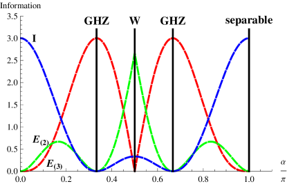
Figure 2: Here the information content in bits of the state ฯฮฑsubscript๐œŒ๐›ผ\rho_{\alpha}, Eq.ย (V), is plotted. The colored, thickened and dashed curves are the single properties I=โˆ‘s=13Ss๐ผsuperscriptsubscript๐‘ 13subscript๐‘†๐‘ I=\sum_{s=1}^{3}S_{s} (blue), the 222โ€“partite entanglement E(2)=E12+E13+E23subscript๐ธ2subscript๐ธ12subscript๐ธ13subscript๐ธ23E_{(2)}=E_{12}+E_{13}+E_{23} (green) and the 333โ€“partite entanglement E(3)=E123subscript๐ธ3subscript๐ธ123E_{(3)}=E_{123} (red). For the GHZโ€“state ฮฑ=ฯ€3/2โ€‹ฯ€3๐›ผ๐œ‹32๐œ‹3\alpha=\frac{\pi}{3}/\frac{2\pi}{3} the 333โ€“partite entanglement is maximal while for the Wโ€“state ฮฑ=ฯ€2๐›ผ๐œ‹2\alpha=\frac{\pi}{2} the 222โ€“partite entanglement is maximal. For ฮฑ=ฯ€6โ€‹5โ€‹ฯ€6๐›ผ๐œ‹65๐œ‹6\alpha=\frac{\pi}{6}\ \frac{5\pi}{6} we obtain another interesting state, the 222โ€“partite entanglement has a second maximum.

Three qubits states: There exist two entangled states, the well known GHZโ€“state and the Wโ€“state, which are obviously in a physically different way entangled. If one traces over one subsystem, in first case one gets a separable state and in the second case an entangled state.

For that let us discuss the states ฯฮฑ=|ฯ•โ€‹(ฮฑ)โŸฉโ€‹โŸจฯ•โ€‹(ฮฑ)|subscript๐œŒ๐›ผketitalic-ฯ•๐›ผbraitalic-ฯ•๐›ผ\rho_{\alpha}=|\phi(\alpha)\rangle\langle\phi(\alpha)| with

|ฯ•โ€‹(ฮฑ)โŸฉketitalic-ฯ•๐›ผ\displaystyle|\phi(\alpha)\rangle =\displaystyle= sinโกฮฑ3โ€‹{|001โŸฉ+|010โŸฉ+|100โŸฉ}+cosโกฮฑโ€‹|111โŸฉ,๐›ผ3ket001ket010ket100๐›ผket111\displaystyle\frac{\sin{\alpha}}{\sqrt{3}}\{|001\rangle+|010\rangle+|100\rangle\}+\cos\alpha\;|111\rangle\;,

which are superposition of the Wโ€“state and a separable state. It is also plotted in Fig.ย 2. For ฮฑ=ฯ€3/2โ€‹ฯ€3๐›ผ๐œ‹32๐œ‹3\alpha=\frac{\pi}{3}/\frac{2\pi}{3} the state is unitary equivalent to the GHZโ€“state (12โ€‹{|000โŸฉ+|111โŸฉ}12ket000ket111\frac{1}{\sqrt{2}}\{|000\rangle+|111\rangle\}). This is at the first side surprising, because the 333โ€“flip and the 222โ€“flip concurrences derive to

C(3)2subscriptsuperscriptC23\displaystyle\textbf{C}^{2}_{(3)} =\displaystyle= 00\displaystyle 0
C(2)2subscriptsuperscriptC22\displaystyle\textbf{C}^{2}_{(2)} =\displaystyle= 83โ€‹(sin4โก(ฮฑ)+3โ€‹cos2โก(ฮฑ)โ€‹sin2โก(ฮฑ)),83superscript4๐›ผ3superscript2๐›ผsuperscript2๐›ผ\displaystyle\frac{8}{3}(\sin^{4}(\alpha)+3\cos^{2}(\alpha)\sin^{2}(\alpha))\;, (25)

i.e. the 333-flip is zero. For the Wโ€“state (ฮฑ=ฯ€2๐›ผ๐œ‹2\alpha=\frac{\pi}{2}) on the other side the 222โ€“flip has a local minimum. These facts suggest that we have to โ€œcorrectโ€ the flip concurrences to obtain the m๐‘šmโ€“partite entanglement in the following way

E(3)subscript๐ธ3\displaystyle E_{(3)} =\displaystyle= E123=C(3)2โ€‹(ฯฮฑ)+C(2)2โ€‹(ฯฮฑ)subscript๐ธ123subscriptsuperscriptC23subscript๐œŒ๐›ผsubscriptsuperscriptC22subscript๐œŒ๐›ผ\displaystyle E_{123}\;=\;\textbf{C}^{2}_{(3)}(\rho_{\alpha})+\textbf{C}^{2}_{(2)}(\rho_{\alpha})
โˆ’{C(2)2โ€‹(Tโ€‹r1โ€‹(ฯฮฑ))+C(2)2โ€‹(Tโ€‹r2โ€‹(ฯฮฑ))+C(2)2โ€‹(Tโ€‹r3โ€‹(ฯฮฑ))}subscriptsuperscriptC22๐‘‡subscript๐‘Ÿ1subscript๐œŒ๐›ผsubscriptsuperscriptC22๐‘‡subscript๐‘Ÿ2subscript๐œŒ๐›ผsubscriptsuperscriptC22๐‘‡subscript๐‘Ÿ3subscript๐œŒ๐›ผ\displaystyle-\{\textbf{C}^{2}_{(2)}\left(Tr_{1}(\rho_{\alpha})\right)+\textbf{C}^{2}_{(2)}(Tr_{2}(\rho_{\alpha}))+\textbf{C}^{2}_{(2)}(Tr_{3}(\rho_{\alpha}))\}
E(2)subscript๐ธ2\displaystyle E_{(2)} =\displaystyle= E12+E13+E23subscript๐ธ12subscript๐ธ13subscript๐ธ23\displaystyle E_{12}+E_{13}+E_{23}
=\displaystyle= C(2)2โ€‹(Tโ€‹r1โ€‹(ฯฮฑ))+C(2)2โ€‹(Tโ€‹r2โ€‹(ฯฮฑ))+C(2)2โ€‹(Tโ€‹r3โ€‹(ฯฮฑ)).subscriptsuperscriptC22๐‘‡subscript๐‘Ÿ1subscript๐œŒ๐›ผsubscriptsuperscriptC22๐‘‡subscript๐‘Ÿ2subscript๐œŒ๐›ผsubscriptsuperscriptC22๐‘‡subscript๐‘Ÿ3subscript๐œŒ๐›ผ\displaystyle\textbf{C}^{2}_{(2)}(Tr_{1}(\rho_{\alpha}))+\textbf{C}^{2}_{(2)}(Tr_{2}(\rho_{\alpha}))+\textbf{C}^{2}_{(2)}(Tr_{3}(\rho_{\alpha}))\;.

It is clear that the sum is unchanged, because we add the sum of the 222โ€“flip concurrence of the reduced density matrices and subtract it. As the 222โ€“flip concurrence of the subsystems are here equivalent to two times the Wootters-Hill concurrence Wootters this sum is clearly invariant under local unitaries. Therefore all that is left to show is that E(3)subscript๐ธ3E_{(3)} cannot get negative. This is easily proven because the entanglement stored in the subsystems can only be lower or at most equivalent to the entanglement stored in the subsystems. This can of course be generalized for mixed states through the convex roof.

With these definitions of the 222โ€“ and 333โ€“partite entanglement we obtain a simple interpretation of the physical difference of the Wโ€“ and the GHZโ€“entanglement. The state ฯฮฑsubscript๐œŒ๐›ผ\rho_{\alpha}, Eq.ย (V), is for ฮฑ=0๐›ผ0\alpha=0 separable, the single property in each subsystem is maximal (see also Fig.ย 2). As ฮฑ๐›ผ\alpha increases the single properties Iโ€‹(ฯฮฑ)=โˆ‘s=13Ss2๐ผsubscript๐œŒ๐›ผsuperscriptsubscript๐‘ 13superscriptsubscript๐‘†๐‘ 2I(\rho_{\alpha})=\sum_{s=1}^{3}S_{s}^{2} have to decrease due to Bohrโ€™s complementary relation (Ss2+Ms2=1superscriptsubscript๐‘†๐‘ 2superscriptsubscript๐‘€๐‘ 21S_{s}^{2}+M_{s}^{2}=1) as their mixednesses increase. For ฮฑ=ฯ€3๐›ผ๐œ‹3\alpha=\frac{\pi}{3} or ฮฑ=2โ€‹ฯ€3๐›ผ2๐œ‹3\alpha=\frac{2\pi}{3} the single properties are zero, thus entanglement is maximal and it is a genuine 333โ€“partite entangled state, the GHZโ€“state. For ฮฑ=ฯ€2๐›ผ๐œ‹2\alpha=\frac{\pi}{2} the 222โ€“partite entanglement is maximal, while the single properties obtain a local maximal and the 333โ€“partite entanglement is zero as desired. There is another interesting state e.g. at ฮฑ=ฯ€6/5โ€‹ฯ€6๐›ผ๐œ‹65๐œ‹6\alpha=\frac{\pi}{6}/\frac{5\pi}{6}, here 222โ€“partite entanglement has another maximum (see Fig.ย 2).

Refer to caption
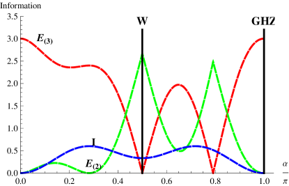
Figure 3: Here the information content in bits of the state ฯ„ฮฑsubscript๐œ๐›ผ\tau_{\alpha}, Eq.ย (27), is plotted. The colored, thickened and dashed curves are the single properties I=โˆ‘s=13Ss๐ผsuperscriptsubscript๐‘ 13subscript๐‘†๐‘ I=\sum_{s=1}^{3}S_{s} (blue), the 222โ€“partite entanglement E(2)=E12+E13+E23subscript๐ธ2subscript๐ธ12subscript๐ธ13subscript๐ธ23E_{(2)}=E_{12}+E_{13}+E_{23} (green) and the 333โ€“partite entanglement E(3)=E123subscript๐ธ3subscript๐ธ123E_{(3)}=E_{123} (red). The single properties I๐ผI are symmetric, however, the genuine 222โ€“ and 333โ€“partite entanglement are not.

Also the above counter example of a biโ€“separable state, Eq.ย (22), obtains the desired interpretation as the 333โ€“partite entanglement E(3)subscript๐ธ3E_{(3)} derives to zero and the 222โ€“partite entanglement to E(2)=E12+E13+E23=2+0+0subscript๐ธ2subscript๐ธ12subscript๐ธ13subscript๐ธ23200E_{(2)}=E_{12}+E_{13}+E_{23}=2+0+0, see also Fig.ย 1ย (d).

In Fig.ย 3 we show the superposition of W and GHZ: ฯ„ฮฑ=|ฯˆโ€‹(ฮฑ)โŸฉโ€‹โŸจฯˆโ€‹(ฮฑ)|subscript๐œ๐›ผket๐œ“๐›ผbra๐œ“๐›ผ\tau_{\alpha}=|\psi(\alpha)\rangle\langle\psi(\alpha)|

|ฯˆโ€‹(ฮฑ)โŸฉket๐œ“๐›ผ\displaystyle|\psi(\alpha)\rangle =\displaystyle= sinโกฮฑ3โ€‹{|001โŸฉ+|010โŸฉ+|100โŸฉ}๐›ผ3ket001ket010ket100\displaystyle\frac{\sin{\alpha}}{\sqrt{3}}\bigl{\{}|001\rangle+|010\rangle+|100\rangle\bigr{\}} (27)
+cosโกฮฑ2โ€‹{|111โŸฉ+|000โŸฉ}.๐›ผ2ket111ket000\displaystyle+\frac{\cos{\alpha}}{\sqrt{2}}\bigl{\{}|111\rangle+|000\rangle\bigr{\}}\;.

The single properties are symmetric, however, the tripartite and the bipartite entanglement depend on the particular superposition. One finds for example another interesting state at (ฮฑ=โ‰ƒ0.8ฯ€\alpha=\simeq 0.8\pi) which maximizes the bipartite entanglement E(2)subscript๐ธ2E_{(2)} while the tripartite entanglement E(3)subscript๐ธ3E_{(3)} is zero (see Fig.ย 3).

For mixed states, if the optimal bounds are known, the m๐‘šmโ€“entanglement derives in the very same way. In Fig.ย 4 we have chosen a mixture of the GHZโ€“state and the Wโ€“state, i.e.

ฯƒโ€‹(ฮฑ)๐œŽ๐›ผ\displaystyle\sigma(\alpha) =\displaystyle= sin2โก(ฮฑ2)โ€‹ฯW+cos2โก(ฮฑ2)โ€‹ฯGโ€‹Hโ€‹Zsuperscript2๐›ผ2subscript๐œŒ๐‘Šsuperscript2๐›ผ2subscript๐œŒ๐บ๐ป๐‘\displaystyle\sin^{2}(\frac{\alpha}{2})\;\rho_{W}+\cos^{2}(\frac{\alpha}{2})\;\rho_{GHZ}\; (28)

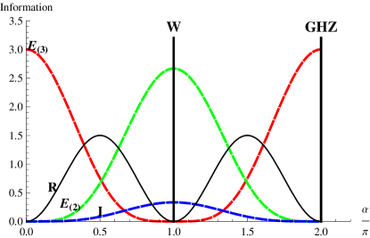
The complementing missing information, due to classical lack of knowledge about the quantum state, Rโ€‹(ฯƒโ€‹(ฮฑ))๐‘…๐œŽ๐›ผR(\sigma(\alpha)), is maximal for ฮฑ=ฯ€2๐›ผ๐œ‹2\alpha=\frac{\pi}{2} as expected.

Refer to caption
Figure 4: Here the information content in bits of the state ฯƒโ€‹(ฮฑ)๐œŽ๐›ผ\sigma(\alpha), Eq.ย (28), is plotted. The colored, thickened and dashed curves are the single properties I=โˆ‘s=13Ss๐ผsuperscriptsubscript๐‘ 13subscript๐‘†๐‘ I=\sum_{s=1}^{3}S_{s} (blue), the 222โ€“partite entanglement E(2)=E12+E13+E23subscript๐ธ2subscript๐ธ12subscript๐ธ13subscript๐ธ23E_{(2)}=E_{12}+E_{13}+E_{23} (green) and the 333โ€“partite entanglement E(3)=E123subscript๐ธ3subscript๐ธ123E_{(3)}=E_{123} (red). The thin, not dashed curve is Rโ€‹(ฯ)๐‘…๐œŒR(\rho), which is the lack of information about the state.

To sum up for 333 qubits we have shown that in a simple and evident way the 222โ€“flip and 333โ€“flip concurrences can be made invariant under local unitaries and these new quantities, the 222โ€“ and 333โ€“partite entanglement, capture then the desired physical differences e.g. of the GHZโ€“state, the Wโ€“state, the biโ€“separable state and of mixed states.

VI The information content of nโ€“partite multidimensional systems

Now returning to the first equation, Eq.ย (1), we see the separation of information in multi-qudit systems: Iโ€‹(ฯ)๐ผ๐œŒI(\rho) quantifies all locally obtainable information as it is just the sum over all obtainable information in every subsystem. Every physical system with d-degrees of freedom can carry one dit of information, which can be separated into predictability and coherence. Of course the combination of n-systems can carry n-dits of information, just as in classical systems. The main difference then is that they cannot all be locally obtained, as for pure entangled systems the sum over all locally obtainable information does not yield n. Here the information is encoded in entanglement, which in itself seems to be separable into different classes of entanglement, as we have seen for the three qubit example. Note that the local information Iโ€‹(ฯ)๐ผ๐œŒI(\rho) is always additive and for the entanglement Eโ€‹(ฯ)๐ธ๐œŒE(\rho) strict additivity is only proven for pure states. For mixed systems only subadditivity of Eโ€‹(ฯ)๐ธ๐œŒE(\rho) can be proven (in the very same way as with entanglement of formation), but additivity is strongly expected (in this case Rโ€‹(ฯ)๐‘…๐œŒR(\rho) can clearly only contain classical uncertainty).

VII Conclusion

We started from Bohrโ€™s complementarity relation, which we generalized for d๐‘‘dโ€“dimensional systems, yielding the information content in every subsystem of a multipartite state ฯ๐œŒ\rho through the single property ๐’ฎsโ€‹(ฯ)subscript๐’ฎ๐‘ ๐œŒ{\cal S}_{s}(\rho). From this relation we are able to consistently quantify the information content in entanglement of pure states as the missing information needed to complement the single properties of all subsystems as nโˆ’โˆ‘s=1n๐’ฎs2โ€‹(ฯ)=โˆ‘s=1nMs2โ€‹(ฯ)๐‘›superscriptsubscript๐‘ 1๐‘›subscriptsuperscript๐’ฎ2๐‘ ๐œŒsuperscriptsubscript๐‘ 1๐‘›subscriptsuperscript๐‘€2๐‘ ๐œŒn-\sum_{s=1}^{n}{\cal S}^{2}_{s}(\rho)=\sum_{s=1}^{n}M^{2}_{s}(\rho). Then we showed that this information can be operationally obtained, thus opening the possibility to derive bounds for the entanglement of multipartite multidimensional systems. Moreover, we have shown that the operations necessary to obtain this measure can be separated into different classes of concurrences, i.e. characterized by the amount of flips m๐‘šm, the m๐‘šmโ€“flip concurrences. Finally that these can be modified to meet our understanding of multipartite entanglement as explicitly shown for three qubits one can correct the m๐‘šmโ€“flip concurrences to m๐‘šmโ€“partite entanglement. This explains the different kind of entanglement of the GHZโ€“state and the Wโ€“state, summarized in Fig.ย 1 and in Fig.ย 2. Moreover, it gives the correct entanglement of any biโ€“separable state. Last but not least we presented a mixed state, where the single properties are complemented by the classical lack of knowledge about the quantum state under investigation. In what way this generalizes for multipartite systems consistently is left for further investigation.

In summary, we found a multidimensional, multipartite and operational entanglement measure which admits a separation into different classes of entanglement and herewith we obtain the information content of any discrete state. This knowledge obviously helps to e.g. decide given a certain state quantum communication or quantum cryptography is possible and to what extend.

Acknowledgement: Thanks to R.A. Bertlmann and Ph. Krammer for enlightening discussions.

References

  • (1) Linden, N., S. Popescu, B. Schumacher, and M. Westmoreland, โ€œReversibility of local transformations of mul- tipartite entanglementโ€, arXiv: quant-ph/9912039.
  • (2) H. Aschauer, W. D r, and H.-J. Briegel, Phys. Rev. A 71, 012319 (2005).
  • (3) W. D r, H. Aschauer, and H.-J. Briegel, Phys. Rev. Lett. 91, 107903 (2003).
  • (4) J. Eisert, H.-J. Briegel, Phys. Rev. A 64, 022306 (2001).
  • (5) A. Borras, A.R. Plastino, J. Batle, C. Zander, M. Casas, and A. Plastino, J. Phys. A: Math. Theor. 40, 13407 (2007).
  • (6) Jian-Ming Cai, Zheng-Wei Zhou, and Guang-Can Guo, โ€œFully multi-qubit entangled statesโ€, arXiv: quant-ph/0609186.
  • (7) David A. Meyer and Nolan R. Wallach, โ€œGlobal entanglement in multiparticle systems Authorsโ€, arXiv: quant-ph/0108104v1.
  • (8) S. Boixo and A. Monras, โ€œAn operational interpretation for global multipartite entanglementโ€, arXiv: quant-ph/0706.2019v2.
  • (9) Ryszard Horodecki, Pawel Horodecki, Michal Horodecki, and Karol Horodecki, โ€œQuantum entanglementโ€, arXiv: quant-ph/0702225v2.
  • (10) Bruss, D., G. M. D Ariano, M. Lewenstein, C. Macchiavello, A. Sen(De), and U. Sen, 2005 โ€œDense coding with multi- partite quantum statesโ€, arXiv:quant-ph/0507146.
  • (11) โ€œScalable multi-particle entanglement of trapped ionsโ€ H. Haeffner, W. Haensel, C. F. Roos, J. Benhelm, D. Chek-al-kar, M. Chwalla, T. Koerber, U. D. Rapol, M. Riebe, P. O. Schmidt, C. Becher, O. G hne, W. D r and R. Blatt, Nature 438, 643 (2005).
  • (12) Almut Beige, Yuan Liang Lim and Christian Schoen, J. Mod. Opt. 54, 397 (2007).
  • (13) D. Greenberger and A. Yasin, Phys. Lett. A 128, 391 (1988).
  • (14) B.-G. Englert, Rev. Lett. 77, 2154 (1996).
  • (15) B. C. Hiesmayr and M. Huber , arXiv:quant-ph/0711.1368., in press: doi:10.1016/j.physleta.2008.02.055.
  • (16) A.ย Bramon, G.ย Garbarino and B.C.ย Hiesmayr, Phys. Rev. A 69, 022112 (2004).
  • (17) B.C. Hiesmayr and V. Vedral, โ€œInterferometric wave-particle duality for thermodynamical systemsโ€, arXiv: quant-ph/0501015.
  • (18) M. Jakob and J. A. Bergou, Phys. Rev. A 76, 052107 (2007).
  • (19) M. Jakob and J.A. Bergou, โ€œQuantitative complementarity relations in bipartite systemsโ€, arXiv: quant-ph/0302075.
  • (20) C.H. Bennett, D.P. DiVincenzo, J.A. Smolin, and W.K. Wootters, Phys. Rev. A 54, 3824 (1996).
  • (21) S. Hill and W.K. Wootters, Phys. Rev. Lett. 78, 5022 (1997).
  • (22) F. Mintert, A.R.R. Carvalho, M. Kus, and A. Buchleitner, Phys. Reports 415, 207 (2005).
  • (23) R. Demkowicz-Dobrzanski, A. Buchleitner, M. Kus, and F. Minert, Phys. Rev. A 74, 052303 (2006).