First determination of the strong coupling constant using NNLO predictions for hadronic event shapes in annihilations
Abstract:
We present the first determination of the strong coupling constant from a fit of next-to-next-to-leading order QCD predictions to event-shape variables, measured in annihilations at LEP. The data have been collected by the ALEPH detector at centre-of-mass energies between 91 and 206 . Compared to results of next-to-leading order fits we observe that the central fit values are lower by about , with considerably reduced scatter among the results obtained with different event-shape variables. The dominant systematic uncertainty from renormalization scale variations is reduced by a factor of two. By combining the results for several event-shape variables and centre-of-mass energies, we find
.
1 Introduction
Quantum Chromodynamics (QCD) is generally accepted to be the correct theory for the description of strong interactions between quarks and gluons [1]. If the quark masses and mixing angles are fixed, then the only free parameter of the theory is the strong coupling constant, . Therefore it is of paramount importance to measure this parameter at the best possible precision. In particular, measurements based on different underlying processes, at different energy scales, constitute an important consistency check of the theory and are used to prove the so-called running of the coupling constant, ie., the decrease of the coupling strength with increasing energy scale [2]. During the last twenty years an enormous wealth of measurements has become available, using many different processes with different initial and final states [3, 4]. These measurements resulted in values for , at different scales , which are perfectly consistent with the expected running of the coupling. When evolved to a single scale, most commonly chosen to be the mass of the Z boson, , the measurements agree with each other within a few percent, and thus can be used to extract a world-average value. The particle data group [4] quotes , which has been improved upon in a more recent global analysis to [5].
Several classes of observables can be identified as useful for an measurement. Inclusive observables, such as the ratio of the cross sections for and or sum rules in deep-inelastic scattering, do not resolve the structure of the hadronic final state. The theoretical predictions are obtained with perturbative QCD (pQCD) and typically known up to next-to-next-to-leading order (NNLO) in the strong coupling constant. Non-perturbative effects related to the transition (hadronisation) of partons (quarks and gluons) to hadrons are strongly suppressed by the scale of the process. Exclusive observables, such as event-shape variables in annihilations, discussed in detail below, resolve topological properties of the hadronic final state and thus are sensitive to gluon radiation. This class of observables shows stronger sensitivity to hadronisation effects, at least in phase-space regions characterised by soft and collinear gluon radiation. Finally, spectroscopic properties of mesons and baryons, such as masses or energy level splittings of heavy quark-antiquark resonances, are necessarily determined by non-perturbative phenomena. Major recent progress in calculations within non-relativistic QCD and lattice QCD has resulted in very precise determinations from this last type of observables [6].
Thanks to the clean initial state and the very large event statistics, annihilations to hadrons at the LEP collider at centre-of-mass energies between 91 and 206 constituted an excellent laboratory for precision tests of QCD in general, and precise measurements of the strong coupling constant in particular [7, 8, 9, 10]. These are complemented by data obtained by the SLD experiment [11] at SLAC at centre-of-mass energy of 91 and by data obtained at the DESY PETRA collider at lower energies, especially the reanalysis of data from the JADE experiment [12].
Many of those measurements were based on event-shape variables such as thrust [13]. These variables probe the structure of the hadronic final state. In the leading-order picture, annihilation to hadrons occurs via and subsequent hadronisation to stable hadrons, resulting in a back-to-back two-jet structure of the event. At the next order of perturbation theory, gluon radiation off quarks will lead to deviations from this two-jet structure due to the appearance of additional jets. In general, event-shape variables quantify the structure of an event by a single measure.
Until recently, pQCD predictions for event-shape observables were known up to next-to-leading order (NLO) in the strong coupling. As a consequence, the residual sensitivity to the choice of the unphysical renormalisation scale, , resulted in systematic uncertainties of the measurements at the 10% level. Those systematic uncertainties are typically estimated by varying over a broad range, eg., , since this variation probes most of the missing higher-order contributions. Using a very large set of event shapes, the DELPHI collaboration observed a large spread in the values extracted from the different observables [14], when fixing . In addition, the measurements preferred rather large values of compared to the world average. On the other hand, simultaneously fitting and the scale resulted in a considerably reduced spread of values, however, at the price of a large spread of preferred parameters, which in addition turned out to be rather small compared to the “natural” choice . Similar observations were made by the other LEP collaborations and on the SLD data [15].
An important part of the missing higher-order contributions was identified to be due to large logarithms in the event-shape variable, related to the incomplete cancellation of real and virtual corrections due to gluon radiation [16, 17, 18, 19, 20, 21]. Once these logarithms are resummed to all orders in pQCD and consistently combined with the fixed-order calculations, the resulting improved predictions lead to a better description of the event-shape variables, most notably close to the two-jet region of the phase space. Consequently, the measurements from fits of these improved predictions were characterised by reduced systematic uncertainties (now at the 5% level) and showed better agreement with other determinations, with typical values in the range . Other systematic uncertainties, from experimental effects and most notably from the estimation of non-perturbative contributions, were smaller than those from the -scale variations. Non-perturbative hadronisation corrections are estimated by either using phenomenological models (string or cluster fragmentation), implemented in Monte Carlo simulations [22, 23, 24], or by adding power-law corrections to the purely perturbative predictions [25].
From all this it became clear that major progress in the pQCD calculations was necessary in order to push the uncertainties of measurements from event shapes below the 5% range, approaching the precision obtained with inclusive observables or lattice calculations. Such major progress has recently been made with the calculation of the NNLO corrections to event-shape variables [26, 27]. Consequently, it is of great interest to include these new corrections in fits for . In this paper we describe first fits of this kind and discuss the results. The measurements are obtained with event-shape distributions measured by the ALEPH experiment [28] at centre-of-mass energies between 91 and 206 . We concentrate on the comparison of the results found at NNLO with those at NLO and NLO matched to resummation of leading and next-to-leading logarithms (NLLA), as used in [28]. In a forthcoming publication results using NNLO matched to NLLA will be discussed in detail.
2 Theoretical predictions
The perturbative expansion for the distribution of a generic observable up to NNLO at centre-of-mass energy , for a renormalisation scale and is given by
| (1) |
Here the event-shape distribution is normalised to the total hadronic cross section . With the assumption of massless quarks we have at NNLO
| (2) |
where the Born cross section for (photon exchange only, with electromagnetic coupling and quark charge ) is
| (3) |
The constant is given by,
| (4) |
where , and the QCD colour factors are
| (5) |
for colours and light quark flavours.
In practice, we use the perturbative coefficients , and , computed in the -scheme in [27], which are all normalised to :
| (6) |
However, , and are straightforwardly related to , and ,
| (7) |
These coefficients are computed at a renormalisation scale fixed to the centre-of-mass energy, and depend therefore only on the value of the observable . They explicitly include only QCD corrections with non-singlet quark couplings and are therefore independent of electroweak couplings. At , these amount to the full corrections, while the corrections also receive a pure-singlet contribution. This pure-singlet contribution arises from the interference of diagrams where the external gauge boson couples to different quark lines. In four-jet observables at , these singlet contributions were found to be extremely small [29].
The QCD coupling constant evolves according to the renormalisation group equation, which is to NNLO:
| (8) |
with the -scheme coefficients
| (9) | |||||
The above equation is solved by introducing as integration constant with , yielding the running coupling constant:
| (10) |
In terms of the running coupling , the NNLO expression for event-shape distributions becomes
| (11) | |||||
The coefficients and have been computed for several event-shape variables [26, 27]. The calculation is carried out using a newly developed parton-level event generator programme EERAD3 which contains the relevant matrix elements with up to five external partons [30, 31, 32, 33]. Besides explicit infrared divergences from the loop integrals, the four-parton and five-parton contributions yield infrared divergent contributions if one or two of the final state partons become collinear or soft. In order to extract these infrared divergences and combine them with the virtual corrections, the antenna subtraction method [34] was extended to NNLO level [35] and implemented for and related event-shape variables [36]. The analytical cancellation of all infrared divergences serves as a very strong check on the implementation. EERAD3 yields the perturbative , and coefficients as histograms for all infrared-safe event-shape variables related to three-particle final states at leading order. As a cross check, the and coefficients have also been obtained from an independent integration [37] of the NLO matrix elements [38], showing excellent agreement. While and can be computed to very high numerical accuracy, the computation of is so CPU-intensive that we could obtain only results with numerical integration errors of typically a few percent. These numerical errors on the -coefficient will be included in the analysis of as described below.
For small values of , the fixed-order expansion, eq. (11), fails to converge, because the fixed-order coefficients are enhanced by powers of , , and . In order to obtain reliable predictions in the region of it is necessary to resum entire sets of logarithmic terms at all orders in . A detailed description of the predictions at next-to-leading-logarithmic approximation (NLLA) can be found in Ref. [39]. There the matching of the NLO and NLLA expressions, which is necessary in order to avoid double counting, is also described. The extension of this matching procedure to NNLO with NNLA is outlined in [17] and will be discussed in detail in a separate publication.
3 Observables and data sets
We have studied the six event-shape distributions thrust [13], heavy jet mass [41], total and wide jet broadening () [42], C-parameter [43] and the Durham jet resolution parameter [44]. The definitions of these variables and a discussion of their properties can be found in Refs. [28] and [39, 40].
The measurements have been carried out by the ALEPH collaboration [28] 111The tables with numbers and uncertainties for all variables can be found at http://aleph.web.cern.ch/aleph/QCD/alephqcd.html., at centre-of-mass energies of 91.2, 133, 161, 172, 183, 189, 200 and 206 . Earlier measurements and complementary data sets from the LEP experiments and from SLD can be found in Refs. [7, 8, 9, 10, 11]. The event-shape distributions were computed using the reconstructed momenta and energies of charged and neutral particles. The measurements have been corrected for detector effects, ie., the final distributions correspond to the so-called particle (or hadron level). The particle level is defined by stable hadrons with a lifetime longer than s after hadronisation and leptons according to the definition given in [47]. In addition, at LEP2 energies above the Z peak they were corrected for initial-state radiation effects. At energies above 133 GeV backgrounds from WW, ZZ and Z were subtracted following the procedure given in [28].
Backgrounds, mainly from W-pair production, were subtracted. The experimental uncertainties were estimated by varying event and particle selection cuts. They are below 1% at LEP1 and slightly larger at LEP2. For further details we refer to Ref. [28].
4 Determination of the strong coupling constant
The coupling constant is determined from a fit of the perturbative QCD predictions to measured event-shape distributions. The procedure adopted here follows closely the one described in Ref. [28]. The six event-shape variables used are , , , , and . The perturbative predictions for the distributions, as described in section 2, are calculated to the same order of perturbation theory for all of these variables. The data set collected by ALEPH at the Z peak with high statistics allows for quantitative comparisons of different pQCD predictions and resulting fits for . The size of missing higher orders, which are inherently difficult to assess, can be different for different variables. Therefore, a combination of measurements using several variables yields a better estimator of than using a single variable. Furthermore, the spread of values of is an independent estimation of the theoretical uncertainty. At centre-of-mass energies above the Z peak the statistical uncertainties are larger and background conditions are more difficult compared to the peak data. Therefore a combination of measurements is particularly important for those energies. We adopt the same combination procedure as described in [28], which is based on weighted averages and takes into account correlations between the event-shape variables. At energies above the measured statistical uncertainties are replaced by expected statistical errors, obtained from a large number of simulated experiments. This avoids biases towards lower values of in the case of small event statistics. The bias originates from larger weights of downward fluctuating bins in the distributions compared to upward fluctuations, as outlined in Ref. [28].
Event-shape distributions are fit in a central region of three-jet production, where a good perturbative description is available. The fit range is placed inside the region where hadronisation and detector corrections are below 25 and the signal-to-background ratio at LEP2 is above one. At the higher LEP2 energies the good perturbative description extends further into the two-jet region, while in the four-jet region the background becomes large. Thus the fit range is selected as a result of an iterative procedure balancing theoretical, experimental and statistical uncertainties. The data are corrected for detector effects, for background from four-fermion processes and for the residual ISR contribution. The background from WW events increases with energy, and after subtraction the content of some bins of the distribution becomes negative. For this reason the fit range is restricted to a region with good signal-to-background ratio.
Since very recently distributions of infrared- and collinear-safe observables at the parton level can be computed in perturbative QCD to third order in , as described in section 2 and in more detail in Ref. [36]. Here we concentrate on fits of NNLO predictions and compare them to pure NLO and matched NLO+NLLA predictions as used in the analysis of Ref. [28]. The nominal value for the renormalisation scale is unity. All these calculations neglect quark masses. Quark mass effects [45] are relevant for the b quark at , where the fraction of events is large, while is still moderate. NLO calculations including a quark mass indicate that the expected change in is of the order of at [46]. The effect is scaling with and decreases to - at 200 GeV. Mass corrections were computed to second order using the matrix elements of [48]. A pole b-quark mass = 5 was used and Standard Model values were taken for the fraction of events. It is worth noting that, since these mass effects are known at NLO only, the NNLO predictions can be corrected only in a partial and not fully consistent manner.
 |
 |
The perturbative QCD prediction is corrected for hadronisation and resonance decays by means of a transition matrix, which is computed with the Monte Carlo generators PYTHIA, HERWIG and ARIADNE, all tuned to global hadronic observables at [47]. The parton level is defined by the quarks and gluons present at the end of the parton shower in PYTHIA and HERWIG and the partons resulting from the color dipole radiation in ARIADNE. Albeit the generators’ limitation to leading-order QCD, a reasonable agreement is observed between the generator parton level and the NNLO prediction inside the fit range within a few percent, as shown in Fig. 1. Corrected measurements of event-shape distributions are compared to the theoretical calculation at particle level.
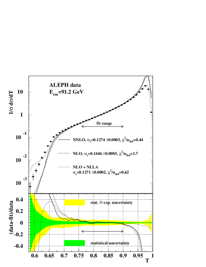
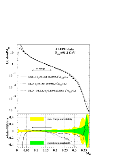
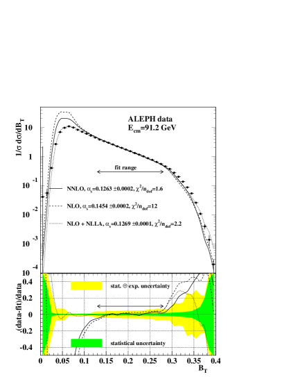
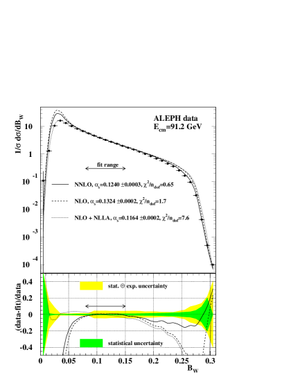
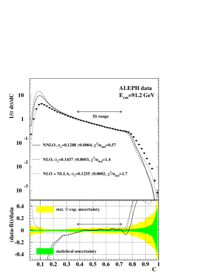
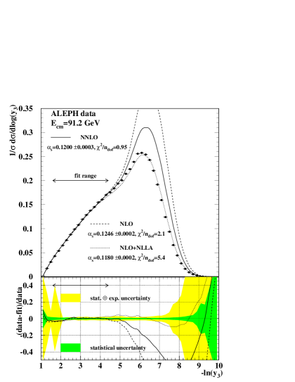
The value of is determined at each energy using a binned least-squares fit. The fit programs of Ref. [28] have been extended to incorporate the NNLO calculations. It has been verified that at NLO+NLLA and using the fit range advocated by ALEPH the results on reported in Ref. [28] are reproduced. Only statistical uncertainties arising from the limited number of observed events, from the number of simulated events used to calculate hadronisation and detector corrections and from the integration procedure of the NNLO coefficient functions are included in the of the fit. Its quality is good for all variables at all energies. Nominal results, based on (1) and using the fitted values of are shown in Figs. 2 and 3 together with the measured distributions. The resulting measurements of are given in Table 1 for 91.2 to 172 GeV and in Table 2 for 183 to 206 GeV.
 |
 |
 |
 |
 |
 |
Furthermore, in Figs. 4 and 5 and in Table 3 we compare the results found when fitting different perturbative predictions to the high-precision data at . In particular we compare the NNLO fits to those obtained with NLO and NLO+NLLA predictions. A detailed description of the latter is given in Ref. [28]. As shown in Figs. 4 and 5 a good description by the NNLO predictions is found for an extended range over the perturbative region compared to NLO. However, in the two-jet region the resummed prediction still yields a better result. Therefore, compared to Ref. [28], the fit range for NNLO and NLO is slightly shifted into the perturbative region. We observe a clear improvement in the fit quality when going to NNLO accuracy. Compared to NLO the value of is lowered by about 10%, but still higher than for NLO+NLLA. Systematic theoretical and experimental uncertainties are discussed in the following section.
| = 91.2 GeV | ||||||
|---|---|---|---|---|---|---|
| variable | ||||||
| 0.1274 | 0.1200 | 0.1261 | 0.1288 | 0.1240 | 0.1263 | |
| stat. error | 0.0003 | 0.0003 | 0.0003 | 0.0004 | 0.0003 | 0.0002 |
| exp. error | 0.0008 | 0.0010 | 0.0011 | 0.0008 | 0.0007 | 0.0007 |
| pert. error | 0.0042 | 0.0039 | 0.0029 | 0.0039 | 0.0029 | 0.0047 |
| hadr. error | 0.0019 | 0.0016 | 0.0044 | 0.0017 | 0.0018 | 0.0018 |
| total error | 0.0047 | 0.0043 | 0.0054 | 0.0043 | 0.0035 | 0.0051 |
| fit range | 0.76-0.90 | 1.6-4.4 | 0.08-0.18 | 0.38-0.72 | 0.08-0.15 | 0.13-0.28 |
| = 133 GeV | ||||||
| variable | ||||||
| 0.1197 | 0.1198 | 0.1216 | 0.1208 | 0.1211 | 0.1177 | |
| stat. error | 0.0035 | 0.0046 | 0.0042 | 0.0030 | 0.0030 | 0.0026 |
| exp. error | 0.0010 | 0.0007 | 0.0011 | 0.0011 | 0.0005 | 0.0012 |
| pert. error | 0.0034 | 0.0034 | 0.0025 | 0.0032 | 0.0022 | 0.0038 |
| hadr. error | 0.0014 | 0.0009 | 0.0028 | 0.0012 | 0.0011 | 0.0014 |
| total error | 0.0052 | 0.0058 | 0.0058 | 0.0047 | 0.0039 | 0.0049 |
| fit range | 0.75-0.94 | 1.6-4.8 | 0.06-0.25 | 0.22-0.75 | 0.05-0.25 | 0.09-0.30 |
| = 161 GeV | ||||||
| variable | ||||||
| 0.1239 | 0.1146 | 0.1267 | 0.1259 | 0.1223 | 0.1231 | |
| stat. error | 0.0054 | 0.0074 | 0.0078 | 0.0046 | 0.0046 | 0.0041 |
| exp. error | 0.0010 | 0.0007 | 0.0011 | 0.0011 | 0.0005 | 0.0012 |
| pert. error | 0.0031 | 0.0032 | 0.0023 | 0.0029 | 0.0020 | 0.0035 |
| hadr. error | 0.0012 | 0.0006 | 0.0022 | 0.0011 | 0.0008 | 0.0013 |
| total error | 0.0064 | 0.0081 | 0.0085 | 0.0056 | 0.0051 | 0.0056 |
| fit range | 0.75-0.94 | 1.2-5.6 | 0.06-0.25 | 0.22-0.75 | 0.05-0.25 | 0.03-0.30 |
| = 172 GeV | ||||||
| variable | ||||||
| 0.1101 | 0.1079 | 0.1095 | 0.1104 | 0.1083 | 0.1125 | |
| stat. error | 0.0072 | 0.0089 | 0.0087 | 0.0064 | 0.0059 | 0.0056 |
| exp. error | 0.0010 | 0.0009 | 0.0011 | 0.0011 | 0.0005 | 0.0012 |
| pert. error | 0.0030 | 0.0032 | 0.0022 | 0.0028 | 0.0019 | 0.0033 |
| hadr. error | 0.0012 | 0.0005 | 0.0021 | 0.0010 | 0.0007 | 0.0012 |
| total error | 0.0079 | 0.0093 | 0.0092 | 0.0069 | 0.0063 | 0.0067 |
| fit range | 0.80-0.96 | 1.2-5.6 | 0.06-0.25 | 0.22-0.75 | 0.05-0.25 | 0.09-0.30 |
| = 183 GeV | ||||||
|---|---|---|---|---|---|---|
| variable | ||||||
| 0.1132 | 0.1070 | 0.1133 | 0.1160 | 0.1114 | 0.1117 | |
| stat. error | 0.0032 | 0.0041 | 0.0039 | 0.0029 | 0.0027 | 0.0027 |
| exp. error | 0.0011 | 0.0009 | 0.0012 | 0.0014 | 0.0005 | 0.0012 |
| pert. error | 0.0029 | 0.0031 | 0.0022 | 0.0027 | 0.0019 | 0.0033 |
| hadr. error | 0.0011 | 0.0004 | 0.0019 | 0.0010 | 0.0007 | 0.0012 |
| total error | 0.0046 | 0.0052 | 0.050 | 0.0043 | 0.0033 | 0.0046 |
| fit range | 0.75-0.94 | 1.2-5.6 | 0.06-0.25 | 0.22-0.75 | 0.05-0.25 | 0.09-0.30 |
| = 189 GeV | ||||||
| variable | ||||||
| 0.1140 | 0.1077 | 0.1118 | 0.1122 | 0.1093 | 0.1124 | |
| stat. error | 0.0020 | 0.0025 | 0.0025 | 0.0017 | 0.0016 | 0.0015 |
| exp. error | 0.0010 | 0.0007 | 0.0013 | 0.0011 | 0.0005 | 0.0013 |
| pert. error | 0.0028 | 0.0031 | 0.0021 | 0.0026 | 0.0018 | 0.0030 |
| hadr. error | 0.0011 | 0.0004 | 0.0018 | 0.0009 | 0.0006 | 0.0012 |
| total error | 0.0037 | 0.0041 | 0.0040 | 0.0034 | 0.0025 | 0.0038 |
| fit range | 0.80-0.96 | 1.6-5.6 | 0.04-0.20 | 0.18-0.60 | 0.04-0.20 | 0.075-0.25 |
| = 200 GeV | ||||||
| variable | ||||||
| 0.1094 | 0.1071 | 0.1079 | 0.1105 | 0.1071 | 0.1082 | |
| stat. error | 0.0022 | 0.0026 | 0.0027 | 0.0018 | 0.0017 | 0.0017 |
| exp. error | 0.0010 | 0.0007 | 0.0014 | 0.0011 | 0.0005 | 0.0013 |
| pert. error | 0.0027 | 0.0031 | 0.0021 | 0.0026 | 0.0018 | 0.0029 |
| hadr. error | 0.0010 | 0.0003 | 0.0017 | 0.0009 | 0.0006 | 0.0011 |
| total error | 0.0037 | 0.0041 | 0.0041 | 0.0035 | 0.0026 | 0.0038 |
| fit range | 0.80-0.96 | 1.6-5.6 | 0.04-0.20 | 0.18-0.60 | 0.04-0.20 | 0.075-0.25 |
| = 206 GeV | ||||||
| variable | ||||||
| 0.1075 | 0.1023 | 0.1093 | 0.1064 | 0.1066 | 0.1056 | |
| stat. error | 0.0021 | 0.0026 | 0.0025 | 0.0017 | 0.0016 | 0.0016 |
| exp. error | 0.0010 | 0.0007 | 0.0011 | 0.0011 | 0.0005 | 0.0012 |
| pert. error | 0.0026 | 0.0031 | 0.0021 | 0.0025 | 0.0017 | 0.0029 |
| hadr. error | 0.0010 | 0.0003 | 0.0016 | 0.0009 | 0.0005 | 0.0011 |
| total error | 0.0037 | 0.0041 | 0.0038 | 0.0034 | 0.0025 | 0.0037 |
| fit range | 0.80-0.96 | 1.6-5.6 | 0.04-0.20 | 0.18-0.60 | 0.04-0.20 | 0.075-0.25 |
 |
 |
 |
 |
 |
 |
| fit range | 0.76 - 0.90 | 0.38 - 0.72 | 0.08 - 0.18 | 0.08 - 0.15 | 0.13 - 0.28 | 1.6-4.4 |
|---|---|---|---|---|---|---|
| NNLO | 0.1274 | 0.1288 | 0.1261 | 0.1240 | 0.1263 | 0.1200 |
| 5.73/13 | 9.07/16 | 10.8/9 | 3.89/6 | 22.6/14 | 14.5/13 | |
| = 0.44 | = 0.57 | = 1.20 | = 0.65 | = 1.61 | = 1.11 | |
| stat.error | 0.0003 | 0.0004 | 0.0003 | 0.0003 | 0.0002 | 0.0003 |
| NLO | 0.1446 | 0.1437 | 0.1353 | 0.1323 | 0.1454 | 0.1246 |
| 1.72 | 1.4 | 4.3 | 1.7 | 11.9 | 2.1 | |
| NLO+NLLA | 0.1271 | 0.1235 | 0.1198 | 0.1164 | 0.1269 | 0.1180 |
| 0.62 | 1.66 | 7.6 | 7.61 | 2.2 | 5.4 |
5 Systematic Uncertainties of
5.1 Experimental Uncertainties
A detailed description of the experimental systematic uncertainties on the measured event-shape distributions is found in Ref. [28]. The resulting uncertainties on the fitted values are estimated in a way similar to that for the event shapes themselves. Changes of the distributions under variations of event and particle selection cuts lead in general to small changes in . In the fit procedure the same expected statistical uncertainties (cf. section 4) are assumed for all variants of the distribution. This procedure reduces purely statistical components in the systematic effect, which are potentially large at LEP2 energies. The total experimental systematic uncertainties of at LEP2 are between 0.5 and 1.5, dominated by limitations of the correction scheme for initial state radiation. Those at LEP1 are below 1 and dominated by imperfections of the simulation of reconstructed neutral hadronic energy deposits. As expected, the experimental uncertainties determined when fitting the NNLO prediction are generally the same as reported by ALEPH using NLO+NLLA fits [28].
5.2 Theoretical Uncertainties
In the case of pure fixed-order predictions, the main source of arbitrariness in the predictions is the choice of the renormalisation scale . The residual dependence of the fitted value of (2) on the renormalisation scale is shown in Fig. 6. A dramatic reduction of the scale dependence by a factor of two is observed when going from NLO to NNLO. But also compared to NLO+NLLA a net improvement is obtained when fitting the NNLO prediction.
 |
 |
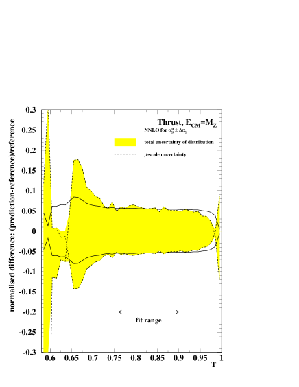
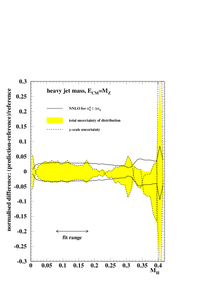
The systematic uncertainty related to missing higher orders is estimated with the uncertainty-band method recommended in Ref. [39]. Briefly, this method derives the uncertainty of from the uncertainty of the theoretical prediction for the event-shape distribution and proceeds in three steps. First a reference perturbative prediction, here NNLO with , is determined using the value of obtained from the combination of the six variables and eight energies, as explained in section 6. Then variants of the prediction with different choices for the scale are calculated with the same value of . In each bin of the distribution for a given variable, the largest upward and downward differences with respect to the reference prediction are taken to define an uncertainty band around the reference theory. In the last step, the value of in the reference prediction is varied, in order to find the range of values which result in predictions lying inside the uncertainty band for the fit range under consideration. In contrast to the original method [39] we do not request the reference prediction to lie strictly inside the uncertainty band, since for the present NNLO calculations the latter is still subject to statistical fluctuations. Instead, we make a fit of the reference theory with as free parameter to the uncertainty band, which includes the statistical uncertainty on the coefficient. The values of fitted to the upper and lower contour of the uncertainty band finally set the perturbative systematic uncertainty. The upward and downward uncertainties are very similar in magnitude and the larger is quoted as symmetric uncertainty. The method is illustrated in Fig. 7, taking thrust and heavy jet mass as examples.
 |
 |
The theoretical error depends on the fit range and on the absolute value of , scaling approximately with at NLO and at NNLO. This behaviour can be seen from (11), where variations of affect all terms, and individual terms compensate each other across the different orders. All compensating terms through , but no compensating terms at are included at NNLO, such that any residual dependence on is to be attributed to these terms.
At LEP2 energies the statistical fluctuations are large. In order to avoid biases from downward fluctuations, the theoretical uncertainties are calculated with the value of obtained by the global combination procedure. For each energy point and in each variable, the error is evolved to the appropriate energy scale and the uncertainty is calculated for the fit range used for the different variables.
The combined value of , used to derive the systematic perturbative error, depends itself on the theoretical error. Hence the procedure of calculating the combination and perturbative error is iterated until convergence is reached, typically after two iterations.
An additional error is evaluated for the b-quark mass correction procedure. This correction has only been calculated to ; no resummed and NNLO expressions are yet available. The difference in obtained with and without mass corrections is taken as systematic error. The total perturbative uncertainty quoted in the tables is the quadratic sum of the errors for missing higher orders and for the mass correction procedure. The total perturbative error is between 3% and 4% at and decreases to between 2% and 3% at LEP2 energies.
The hadronisation model uncertainty is estimated by comparing the standard hadron-level event generator programs HERWIG and ARIADNE to PYTHIA for both hadronisation and detector corrections. The same set of corrections as in Ref. [28] is used. Both corrections are calculated with the same generator in order to obtain a coherent description at the hadron level. The maximum change with respect to the nominal result using PYTHIA is taken as systematic error. It was verified that calculating the detector corrections and the hadronization corrections with different event generator programs yields consistent results. At LEP2 energies the hadronisation model uncertainty is again subject to statistical fluctuations. These fluctuations are observed from one energy to the next and originate from limited statistics of the fully simulated detector-correction functions. Since non-perturbative effects are expected to decrease with , the energy evolution of hadronisation errors has been fitted to a simple parametrisation. The fit was performed for each variable separately. In the fit procedure a weight scaling with luminosity is assigned to the hadronisation uncertainty at each energy point. This ensures that the hadronisation uncertainty at , which is basically free of statistical fluctuations, is not altered by the procedure. As in the case of experimental systematic uncertainties, the hadronisation uncertainty is essentially identical to that published in [28].
The perturbative component of the error, which is the dominant source of uncertainty in most cases, is highly correlated between the energy points. The perturbative errors decrease with increasing , and faster than the coupling constant itself. The overall error is in general dominated by the renormalisation scale dependence.
6 Combined Results
The measurements obtained with the six different variables are combined into a single measurement per energy using weighted averages. The same procedure as in [28] is applied here and it was verified that the combined results using NLO+NLLA with the fit range and weights reported in [28] can be reproduced. A weight is assigned to each observable-dependent measurement proportional to the inverse square of its total error, . The weighted average is then given by
and the combined statistical error is
for which the correlation coefficients are needed. This correlation between fits of to different variables is obtained using a large number of simulated data samples and turns out to be typically 60–80 (cf. Ref. [28]). The correlation of systematic errors is taken into account by recomputing the weighted average for all variations of the analysis, and the change in with respect to the nominal value is taken as error.
| GeV | 91.2 | 133 | 161 | 172 | 183 | 189 | 200 | 206 |
|---|---|---|---|---|---|---|---|---|
| 0.1252 | 0.1202 | 0.1231 | 0.1099 | 0.1122 | 0.1110 | 0.1082 | 0.1064 | |
| stat. error | 0.0002 | 0.0023 | 0.0036 | 0.0048 | 0.0021 | 0.0013 | 0.0014 | 0.0013 |
| exp. error | 0.0008 | 0.0009 | 0.0009 | 0.0009 | 0.0009 | 0.0009 | 0.0009 | 0.0009 |
| pert. error | 0.0037 | 0.0030 | 0.0028 | 0.0027 | 0.0026 | 0.0024 | 0.0024 | 0.0023 |
| hadr. error | 0.0018 | 0.0012 | 0.0009 | 0.0009 | 0.0008 | 0.0008 | 0.0007 | 0.0007 |
| total error | 0.0042 | 0.0041 | 0.0047 | 0.0057 | 0.0035 | 0.0030 | 0.0030 | 0.0029 |
| RMS | 0.0031 | 0.0014 | 0.0043 | 0.0017 | 0.0030 | 0.0023 | 0.0013 | 0.0023 |
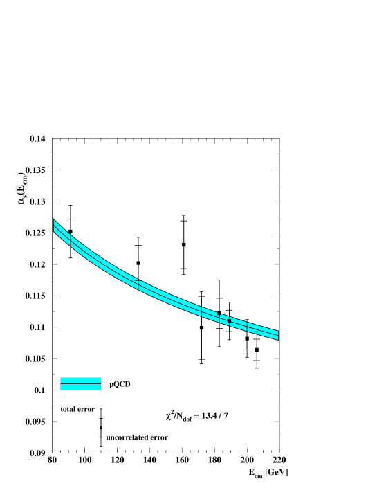
The combination of experimental systematic uncertainties at LEP2 energies is obtained using a luminosity-weighted average of the uncertainties between 133 GeV and 206 GeV. Combined results are given in Table 4, where RMS denotes the root mean squared between the different observables. They are shown in Fig. 8, together with a fit of the QCD expectation. The curve is seen to be in good agreement with the measurements. In the definition of the of the fit only the uncorrelated component of the errors is taken into account, which excludes the perturbative error.
The combined measurements between 133 and 206 GeV are evaluated at the scale of the Z boson mass by using the predicted energy evolution of the coupling constant, eq. (10). The measurements evolved to are given in Table 5. They are again combined using a weighted average, with weights proportional to the inverse square of the total uncertainties. In contrast to the combination from different variables, here the measurements are statistically uncorrelated. Correlations between systematic uncertainties are taken into account and all variations of the determination of have been performed for the weighted average.
| GeV | 91.2 | 133 | 161 | 172 | 183 | 189 | 200 | 206 |
|---|---|---|---|---|---|---|---|---|
| 0.1252 | 0.1276 | 0.1352 | 0.1207 | 0.1247 | 0.1238 | 0.1215 | 0.1196 | |
| stat. error | 0.0002 | 0.0026 | 0.0043 | 0.0058 | 0.0026 | 0.0016 | 0.0017 | 0.0017 |
| exp. error | 0.0008 | 0.0011 | 0.0012 | 0.0012 | 0.0012 | 0.0011 | 0.0011 | 0.0011 |
| pert. error | 0.0037 | 0.0032 | 0.0030 | 0.0030 | 0.0028 | 0.0027 | 0.0027 | 0.0027 |
| hadr. error | 0.0018 | 0.0013 | 0.0011 | 0.0011 | 0.0010 | 0.0009 | 0.0009 | 0.0009 |
| total error | 0.0042 | 0.0045 | 0.0055 | 0.0067 | 0.0041 | 0.0035 | 0.0035 | 0.0035 |
| RMS | 0.0031 | 0.0015 | 0.0053 | 0.0020 | 0.0037 | 0.0029 | 0.0017 | 0.0029 |
The final result is , and the error components are given in Table 6. Included in Table 6 is the combination of measurements at LEP2 energies without the point at . The total uncertainty of the combined LEP2 measurements is smaller than the uncertainty of the LEP1 measurement, because the dominant perturbative uncertainties are reduced at higher energies, even after evolution to .
| data set | LEP1 + LEP2 | LEP2 |
|---|---|---|
| 0.1240 | 0.1238 | |
| stat. error | 0.0008 | 0.0009 |
| exp. error | 0.0010 | 0.0011 |
| pert. error | 0.0029 | 0.0028 |
| hadr. error | 0.0011 | 0.0010 |
| total error | 0.0033 | 0.0033 |
7 Discussion
The improvements achieved by the NNLO fit compared to that at NLO are twofold. First, the renormalisation scale uncertainty on the extracted value of is significantly reduced. This is clearly illustrated in Fig. 6 by comparing the NNLO (solid) and NLO (dashed) curves, in the case of thrust and heavy jet mass. Similar improvements are obtained for the other variables. Second, we find a better description of the event-shape distributions over a larger range. This is evident in Figs. 4 and 5.
Of course, we also have to perform a careful comparison of the NNLO results with those found in NLO+NLLA analyses, which were the state of the art during the LEP era. Once again, Fig. 6 shows that the NNLO perturbative uncertainty is reduced by about 30% compared to NLO+NLLA.
It is also remarkable that the values obtained from fits to different event shapes with NNLO predictions are considerably more self-consistent than those found with either NLO or NLO+NLLA expansions. Not only are the extracted values of more precise, but the spread obtained from the different observables is smaller. This is clearly shown for the data set at in Fig. 9. The key to this dramatic improvement is the rather different size of the NNLO corrections to the various observables.
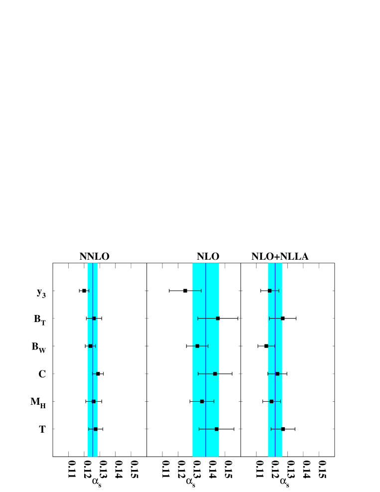
Despite these improvements our final combined result on still appears to be larger than the world average [5]. We recall that the value of obtained from fits with NLO+NLLA predictions is smaller than that obtained with pure NLO calculations alone. Here we observe that when going from NLO to NNLO there is also a trend in the direction of lower values of .
Clearly, resummed predictions are mandatory in the two-jet region. Figures 4 and 5 clearly show the improvement achieved with NLO+NLLA predictions in the two-jet region. Measurements of using NLO+NLLA approximations profit from an extended fit range in this region. While a consistent matching of NNLLA predictions to NNLO would require the analytic resummation of next-to-next-to-leading logarithmic terms, which are not known at present, a matching of existing NLLA expressions to the NNLO calculations requires only the calculation of certain matching coefficients [49]. In this case also a better description in the two-jet region can be expected. First preliminary results have been obtained by us with such matched NNLO+NNLA predictions and fits to data seem to confirm the expected trend towards lower values of . We will address this issue in a forthcoming publication.
Electroweak corrections may also be of a similar size as the NNLO corrections discussed here. At present, these corrections are only known for the inclusive observables like the hadronic cross section [50], where they are found to be sizeable [51], but not for the event-shape distributions. This issue deserves further study and will also be addressed in a forthcoming publication.
8 Conclusions
In this paper we used the newly derived NNLO QCD corrections to event shapes in e+e- annihilation [26, 27] to perform the first determination of the strong coupling constant from event-shape data at NNLO. Our analysis is based on the full set of event-shape distributions measured by the ALEPH collaboration [28] at LEP1 and LEP2.
We observe that the inclusion of NNLO QCD corrections to the different shape variables yields several important effects, when compared to the previously available determinations of , based either on pure NLO calculations or NLO predictions matched to NLL approximations :
-
(a)
The dominant theoretical uncertainty on , as estimated from scale variations, is reduced by a factor 2 (1.3) compared to NLO (NLO+NLLA). A further improvement can be anticipated from a matching of NNLO and NLLA predictions.
-
(b)
The central value obtained at NNLO,
,
is about 10% lower than at NLO, and therefore closer to, albeit still larger than, the world average from other observables. It is also larger than the central value obtained at NLO+NLLA [28], which shows the obvious need for a matching of NNLO+NLLA for a fully reliable result.
-
(c)
The scatter among the values of extracted from the six different event-shape variables is reduced very substantially at NNLO. This is a clear indication that this scatter was largely due to missing higher order perturbative corrections in previous studies.
These observations visibly illustrate the improvements gained from the inclusion of the NNLO corrections, and highlight the need for further studies on the matching of NNLO+NLLA, on the derivation of NNLLA resummation terms, and on the electroweak corrections to event shapes in e+e- annihilation.
Acknowledgements
This research was supported in part by the Swiss National Science Foundation (SNF) under contract 200020-117602, by the UK Science and Technology Facilities Council and by the European Commision’s Marie-Curie Research Training Network under contract MRTN-CT-2006-035505 “Tools and Precision Calculations for Physics Discoveries at Colliders”.
References
-
[1]
R.K. Ellis, W.J. Stirling and B.R. Webber, QCD and Collider Physics,
Cambridge University Press (Cambridge, 1996);
G. Dissertori, I.G. Knowles and M. Schmelling, Quantum Chromodynamics: High Energy Experiments and Theory, Oxford University Press (Oxford, 2003). -
[2]
D.J. Gross and F. Wilczek, Phys. Rev. D8 (1973) 3633;
H.D. Politzer, Phys. Rept. 14 (1974) 129. -
[3]
O. Biebel,
Phys. Rept. 340 (2001) 165;
S. Kluth, Rept. Prog. Phys. 69 (2006) 1771 [hep-ex/0603011]. - [4] W. M. Yao et al. [Particle Data Group], J. Phys. G 33 (2006) 1.
- [5] S. Bethke, Prog. Part. Nucl. Phys. 58 (2007) 351 [hep-ex/0606035].
-
[6]
Q. Mason et al. [HPQCD Collaboration],
Phys. Rev. Lett. 95 (2005) 052002
[hep-lat/0503005];
M. Göckeler, R. Horsley, A.C. Irving, D. Pleiter, P.E.L. Rakow, G. Schierholz and H. Stuben, Phys. Rev. D 73 (2006) 014513 [hep-ph/0502212];
N. Brambilla, X. Garcia i Tormo, J. Soto and A. Vairo, Phys. Rev. D 75 (2007) 074014 [hep-ph/0702079]. -
[7]
D. Buskulic et al. [ALEPH Collaboration],
Z. Phys. C 73 (1997) 409.
-
[8]
P.D. Acton et al. [OPAL Collaboration],
Z. Phys. C 59 (1993) 1;
G. Alexander et al. [OPAL Collaboration], Z. Phys. C 72 (1996) 191;
K. Ackerstaff et al. [OPAL Collaboration], Z. Phys. C 75 (1997) 193;
G. Abbiendi et al. [OPAL Collaboration], Eur. Phys. J. C 16 (2000) 185 [hep-ex/0002012];
G. Abbiendi et al. [OPAL Collaboration], Eur. Phys. J. C 40 (2005) 287 [hep-ex/0503051]. -
[9]
M. Acciarri et al. [L3 Collaboration],
Phys. Lett. B 371 (1996) 137;
M. Acciarri et al. [L3 Collaboration], Phys. Lett. B 404 (1997) 390;
M. Acciarri et al. [L3 Collaboration], Phys. Lett. B 444 (1998) 569;
P. Achard et al. [L3 Collaboration], Phys. Lett. B 536 (2002) 217 [hep-ex/0206052];
P. Achard et al. [L3 Collaboration], Phys. Rept. 399 (2004) 71 [hep-ex/0406049]. -
[10]
P. Abreu et al. [DELPHI Collaboration],
Phys. Lett. B 456 (1999) 322;
J. Abdallah et al. [DELPHI Collaboration], Eur. Phys. J. C 29 (2003) 285 [hep-ex/0307048];
J. Abdallah et al. [DELPHI Collaboration], Eur. Phys. J. C 37 (2004) 1 [hep-ex/0406011]. - [11] K. Abe et al. [SLD Collaboration], Phys. Rev. D 51 (1995) 962 [hep-ex/9501003].
-
[12]
P.A. Movilla Fernandez, O. Biebel, S. Bethke, S. Kluth and
P. Pfeifenschneider [JADE Collaboration],
Eur. Phys. J. C 1 (1998) 461
[hep-ex/9708034];
P. Pfeifenschneider et al. [JADE collaboration], Eur. Phys. J. C 17 (2000) 19 [hep-ex/0001055]. -
[13]
S. Brandt C. Peyrou, R. Sosnowski and A. Wroblewski, Phys. Lett. 12 (1964) 57;
E. Farhi, Phys. Rev. Lett. 39 (1977) 1587. - [14] P. Abreu et al. [DELPHI Collaboration], Eur. Phys. J. C 14 (2000) 557 [hep-ex/0002026].
- [15] P. N. Burrows, H. Masuda, D. Muller and Y. Ohnishi, Phys. Lett. B 382 (1996) 157 [arXiv:hep-ph/9602210].
-
[16]
S. Catani, G. Turnock, B. R. Webber and L. Trentadue,
Phys. Lett. B 263 (1991) 491;
S. Catani, G. Turnock and B. R. Webber, Phys. Lett. B 272 (1991) 368. - [17] S. Catani, L. Trentadue, G. Turnock and B. R. Webber, Nucl. Phys. B 407 (1993) 3.
- [18] G. Dissertori and M. Schmelling, Phys. Lett. B 361 (1995) 167.
-
[19]
S. Catani, G. Turnock and B. R. Webber,
Phys. Lett. B 295 (1992) 269;
Y. L. Dokshitzer, A. Lucenti, G. Marchesini and G. P. Salam, JHEP 9801 (1998) 011 [hep-ph/9801324]. - [20] S. Catani and F. Hautmann, Nucl. Phys. B 427 (1994) 475 [hep-ph/9405388].
- [21] A. Banfi, G. P. Salam and G. Zanderighi, JHEP 0201 (2002) 018 [hep-ph/0112156].
- [22] T. Sjostrand, P. Eden, C. Friberg, L. Lönnblad, G. Miu, S. Mrenna and E. Norrbin, Comput. Phys. Commun. 135 (2001) 238 [hep-ph/0010017].
- [23] G. Corcella et al., JHEP 0101 (2001) 010 [hep-ph/0011363].
- [24] L. Lönnblad, Comput. Phys. Commun. 71 (1992) 15.
-
[25]
B.R. Webber,
Phys. Lett. B 339 (1994) 148
[hep-ph/9408222];
Y.L. Dokshitzer and B.R. Webber, Phys. Lett. B 352 (1995) 451 [hep-ph/9504219]; Phys. Lett. B 404 (1997) 321 [hep-ph/9704298];
Y.L. Dokshitzer, G. Marchesini and B.R. Webber, Nucl. Phys. B 469 (1996) 93 [hep-ph/9512336];
E. Gardi and L. Magnea, JHEP 0308 (2003) 030 [hep-ph/0306094];
E. Gardi and J. Rathsman, Nucl. Phys. B 638 (2002) 243 [hep-ph/0201019];
G.P. Salam and D. Wicke, JHEP 0105 (2001) 061 [hep-ph/0102343]. - [26] A. Gehrmann-De Ridder, T. Gehrmann, E.W.N. Glover and G. Heinrich, Phys. Rev. Lett. 99 (2007) 132002 [arXiv:0707.1285].
- [27] A. Gehrmann-De Ridder, T. Gehrmann, E.W.N. Glover and G. Heinrich, JHEP 0712 (2007) 094 [arXiv:0711.4711].
- [28] A. Heister et al. [ALEPH Collaboration], Eur. Phys. J. C 35 (2004) 457.
- [29] L.J. Dixon and A. Signer, Phys. Rev. Lett. 78 (1997) 811 [hep-ph/9609460]; Phys. Rev. D 56 (1997) 4031 [hep-ph/9706285].
- [30] L.W. Garland, T. Gehrmann, E.W.N. Glover, A. Koukoutsakis and E. Remiddi, Nucl. Phys. B 627 (2002) 107 [hep-ph/0112081] and 642 (2002) 227 [hep-ph/0206067].
- [31] S. Moch, P. Uwer and S. Weinzierl, Phys. Rev. D 66 (2002) 114001 [hep-ph/0207043].
-
[32]
E.W.N. Glover and D.J. Miller,
Phys. Lett. B 396 (1997) 257
[hep-ph/9609474];
Z. Bern, L.J. Dixon, D.A. Kosower and S. Weinzierl, Nucl. Phys. B 489 (1997) 3 [hep-ph/9610370];
J.M. Campbell, E.W.N. Glover and D.J. Miller, Phys. Lett. B 409 (1997) 503 [hep-ph/9706297];
Z. Bern, L.J. Dixon and D.A. Kosower, Nucl. Phys. B 513 (1998) 3 [hep-ph/9708239]. -
[33]
K. Hagiwara and D. Zeppenfeld, Nucl. Phys. B 313 (1989) 560;
F.A. Berends, W.T. Giele and H. Kuijf, Nucl. Phys. B 321 (1989) 39;
N.K. Falck, D. Graudenz and G. Kramer, Nucl. Phys. B 328 (1989) 317. -
[34]
D.A. Kosower,
Phys. Rev. D 57 (1998) 5410
[hep-ph/9710213];
Phys. Rev. D 71 (2005) 045016
[hep-ph/0311272];
J. Campbell, M.A. Cullen and E.W.N. Glover, Eur. Phys. J. C 9 (1999) 245 [hep-ph/9809429]. - [35] A. Gehrmann-De Ridder, T. Gehrmann and E.W.N. Glover, JHEP 0509 (2005) 056 [hep-ph/0505111]; Nucl. Phys. B 691 (2004) 195 [hep-ph/0403057]; Phys. Lett. B 612 (2005) 36 [hep-ph/0501291]; 612 (2005) 49 [hep-ph/0502110].
- [36] A. Gehrmann-De Ridder, T. Gehrmann, E.W.N. Glover and G. Heinrich, JHEP 0711 (2007) 058 [arXiv:0710.0346].
- [37] Z. Kunszt and P. Nason, in Z Physics at LEP 1, CERN Yellow Report 89-08, Vol. 1, p. 373; S. Catani and M. H. Seymour, Phys. Lett. B 378 (1996) 287 [hep-ph/9602277].
- [38] R.K. Ellis, D.A. Ross and A.E. Terrano, Nucl. Phys. B 178 (1981) 421.
- [39] R.W.L. Jones, M. Ford, G.P. Salam, H. Stenzel and D. Wicke, JHEP 0312 (2003) 007 [hep-ph/0312016].
- [40] M. Dasgupta and G.P. Salam, J. Phys. G 30 (2004) R143 [hep-ph/0312283].
- [41] L. Clavelli and D. Wyler, Phys. Lett. B 103 (1981) 383.
- [42] P.E.L. Rakow and B.R. Webber, Nucl. Phys. B 191 (1981) 63.
-
[43]
G. Parisi,
Phys. Lett. B 74 (1978) 65;
J.F. Donoghue, F.E. Low and S.Y. Pi, Phys. Rev. D 20 (1979) 2759. -
[44]
S. Catani, Y.L. Dokshitzer, M. Olsson, G. Turnock and B.R. Webber,
Phys. Lett. B 269 (1991) 432;
N. Brown and W. J. Stirling, Phys. Lett. B 252 (1990) 657; Z. Phys. C 53 (1992) 629. W.J. Stirling et al., Proceedings of the Durham Workshop, J. Phys. G17 (1991) 1567;
S. Bethke, Z. Kunszt, D. E. Soper and W. J. Stirling, Nucl. Phys. B 370 (1992) 310 [Erratum-ibid. B 523 (1998) 681]. - [45] S. Schumann and F. Krauss, arXiv:0709.1027 [hep-ph].
- [46] R. Barate et al. [ALEPH Collaboration], Eur. Phys. J. C 18 (2000) 1 [hep-ex/0008013].
- [47] R. Barate et al. [ALEPH Collaboration], Phys. Rep. 294 (1998) 1.
-
[48]
W. Bernreuther, A. Brandenburg and P. Uwer,
Phys. Rev. Lett. 79 (1997) 189
[hep-ph/9703305];
A. Brandenburg and P. Uwer, Nucl. Phys. B 515 (1998) 279 [hep-ph/9708350];
G. Rodrigo, A. Santamaria and M. S. Bilenky, Phys. Rev. Lett. 79 (1997) 193 [hep-ph/9703358];
P. Nason and C. Oleari, Nucl. Phys. B 521 (1998) 237 [hep-ph/9709360]. - [49] T. Gehrmann and G. Luisoni, in preparation.
- [50] D.Y. Bardin, P. Christova, M. Jack, L. Kalinovskaya, A. Olchevski, S. Riemann and T. Riemann, Comput. Phys. Commun. 133 (2001) 229 [hep-ph/9908433].
- [51] H. Stenzel, JHEP 0507 (2005) 0132 [hep-ph/0501245].