Computing High Accuracy Power Spectra with Pico

Abstract

This paper presents the second release of Pico (Parameters for the Impatient COsmologist). Pico is a general purpose machine learning code which we have applied to computing the CMB power spectra and the WMAP likelihood. For this release, we have made improvements to the algorithm as well as the data sets used to train Pico, leading to a significant improvement in accuracy. For the $9$ parameter nonflat case presented here Pico can on average compute the TT, TE and EE spectra to better than $1\%$ of cosmic standard deviation for nearly all $\ell$ values over a large region of parameter space. Performing a cosmological parameter analysis of current CMB and large scale structure data, we show that these power spectra give very accurate $1$ and $2$ dimensional parameter posteriors. We have extended Pico to allow computation of the tensor power spectrum and the matter transfer function. Pico runs about $1500$ times faster than CAMB at the default accuracy and about $250,000$ times faster at high accuracy. Training Pico can be done using massively parallel computing resources, including distributed computing projects such as Cosmology@Home. On the homepage for Pico, located at http://cosmos.astro.uiuc.edu/pico, we provide new sets of regression coefficients and make the training code available for public use.

1. Introduction

Given the quantity of data available from current experiments such as WMAP and SDSS as well as the prospects for the next generation Planck and DES experiments on the horizon, there is growing need for cosmologists to develop tools that can accurately interpret the flood of data these experiments will gather. A key component in all such analysis is the exploration of the posterior density of the cosmological parameters given the available data. This allows us to constrain and test theoretical models of the Universe. A major computational hurdle in this procedure is the ability to quickly and accurately compute the power spectrum of CMB fluctuations and the matter transfer function. This is accomplished using codes such as CMBFast (Seljak & Zaldarriaga, 1996) and CAMB (Lewis et al., 2000) that evolve the Boltzmann equation for the various constituents of the Universe. Using the default accuracy settings in CAMB the calculation of a single power spectrum takes on the order of a minute. At higher settings, as may be required by upcoming CMB experiments, the computational time can jump to several hours on a modern desktop. Furthermore, computation of constraints based on the data requires evaluating the power spectrum at $\mathcal{O}\left(10^{5}-10^{6}\right)$ models. Decreasing the time required to calculate the CMB power spectrum, while maintaining sub-cosmic variance accuracy, will play an important part of turning raw data into quantitative information about the history and structure of the Universe.

Previous codes aimed at speeding up power spectrum computations such as DASH (Kaplinghat et al., 2002) and CMBwarp (Jimenez et al., 2004) have attempted to reproduce the computation of CMBFast or CAMB. More recently, motivated to develop a code that was both faster than DASH and more accurate than CMBwarp, we released a machine learning code called Pico (Fendt & Wandelt, 2007). It uses a training set of power spectra from CAMB to fit several multivariate polynomials as a function of the input parameters. Along with accurately fitting the power spectra, we also found that Pico was able to directly fit the WMAP likelihood (Spergel et al., 2007; Hinshaw et al., 2007; Page et al., 2007). This was done previously by CMBFit (Sandvik et al., 2004) which used a similar idea of fitting the likelihood with a polynomial in the cosmological parameters. By replacing CAMB and the WMAP likelihood code with Pico we demonstrated that it can quickly explore the parameter space and give nearly identical posteriors. Since the first release of Pico, Auld et al. have applied a neural network code called CosmoNet to flat (Auld et al., 2006) and nonflat (Auld et al., 2007) models. Also Habib et al. have demonstrated that a Gaussian process model introduced in (Heitmann et al., 2006) can predict the CMB power spectrum for flat models based on a very small training set (Habib et al., 2007). Here we discuss some improvements to increase the accuracy of Pico and extend its to application to more general cosmological models. Further, we describe a training method that avoids serial runs of CAMB and is designed to leverage access to massively parallel and even distributed computing resources. For example, we demonstrate that Pico can be trained using the thousands of geographically distinct hosts that contribute to Cosmology@Home.

This paper is organized as follows. Section 2 summarizes some of the improvements to the Pico algorithm and how training sets are generated. In section 3 we demonstrate the performance of Pico in computing the power spectrum, matter transfer function and WMAP likelihood for a $9$ parameter nonflat model. We show that Pico can be used to quickly explore the parameter posterior for this model while accurately reproducing the $1$ and $2$ dimensional marginalized distributions. Lastly we summarize and conclude in section 4.

2. The Algorithm

2.1. Overview

Given a training set of Cosmological parameters $\mathbf{x}$ and CMB power spectra $\mathbf{y}$, Pico models the function $\mathbf{y}=f\left(\mathbf{x}\right)$ in $3$ steps. First it compresses the power spectra using a Karhunen-Loève (Karhunen, 1946; Loève, 1955; Tegmark & Bunn, 1995) technique. For $\ell_{\mathrm{max}}=3000$, the temperature and polarization spectra due to scalar and tensor perturbations can be compressed to $\sim 180$ total numbers. Next the algorithm clusters the input parameters into non-overlapping regions. This is done using a $k$-means algorithm (MacQueen, 1967; Kirby, 2001) or by choosing hyperplanes to manually partition the space. Lastly, Pico models the function by fitting a least-squares polynomial to the compressed power spectra over each cluster. Details of the algorithm can be found in the appendix of Fendt & Wandelt (2007).

2.2. Improved Fitting

The first change to the algorithm is that it now uses the LAPACK libraries to perform matrix decomposition. LAPACK makes the algorithm more stable, allowing the use of higher order polynomials. This gives Pico better fits at low $\ell$ ($<200$) and high $\ell$ ($>1500$). This also makes clustering significantly less important but still useful for improving the low $\ell$ accuracy as well as improving the fit to the WMAP likelihood directly. In particular, we have found that partitioning the training set along values of constant $\Omega_{\mathrm{k}}$ improves the low $\ell$ accuracy in the temperature power spectrum and matter transfer function, while partitioning in $\tau$, the reionization depth, gives a large improvement in computing the polarization power spectrum at low $\ell$.

2.3. Decreasing Numerical Noise

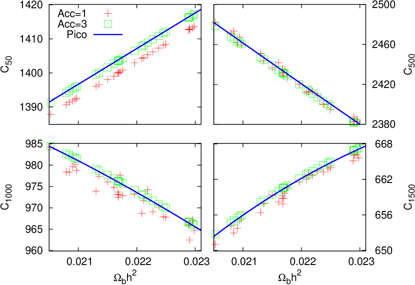
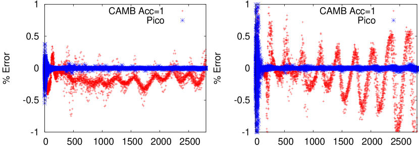
For nonflat models, fitting algorithms are hindered by the fact that at the default accuracy the power spectra computed by CAMB are numerically noisy. This is demonstrated in Figure 1, where we have plotted the power spectrum at the default and high accuracy levels for various $\ell$-values as a function of a single parameter ($\Omega_{\mathrm{b}}h^{2}$) for a nonflat model. Since the power spectrum is not a numerically smooth function of the cosmological parameters, Pico is limited in its ability to fit the true spectra. Also note that the higher accuracy power spectrum does not always smooth over the lower accuracy case. To reduce this noise and limit the effect of interpolation errors we have generated training sets with CAMB using the accuracy parameters set as: Accuracy=3, lAccuracy=3 and lSamp=3. In Figure 2 we have plotted the error between the default and high accuracy power spectra from CAMB for $25$ models around the peak of the WMAP likelihood. The left and right plots show the percent error in the TT and EE spectra. Also shown is the error between the spectra computed by Pico and the high accuracy CAMB runs. Here Pico was trained on the $9$ parameter model discussed in section 3. The figures demonstrate that when trained on high accuracy data Pico computes the power spectrum around the peak of the likelihood to better precision than CAMB at its default accuracy settings.

Figure 1.— The plot shows the value of the temperature spectrum as a function of $\Omega_{\mathrm{b}}h^{2}$ at various $\ell$-values for a nonflat cosmology. The red ($+$) points correspond to to the default CAMB accuracies ($1$,$1$,$1$) and the green ($\Box$) points correspond to higher accuracy settings ($3$,$3$,$1$). While at low $\ell$ the power spectrum is smooth, the default accuracy becomes numerically noisy at higher $\ell$. This is one reason adding $\Omega_{\mathrm{k}}$ as a free parameter increases the difficulty in fitting the power spectrum. Also plotted, as a blue line, is the power spectrum computed by Pico trained on the $9$ parameter nonflat model discussed in section 3.

Figure 2.— The plots show the percent error between the TT (left) and EE (right) power spectrum computed by CAMB at the default accuracy compared to those computed at high accuracy . Also shown is the percent error between the power spectra computed by Pico and the high accuracy CAMB spectra. This test was done on $25$ models all located within $25$ log-likelihoods of the WMAP peak.

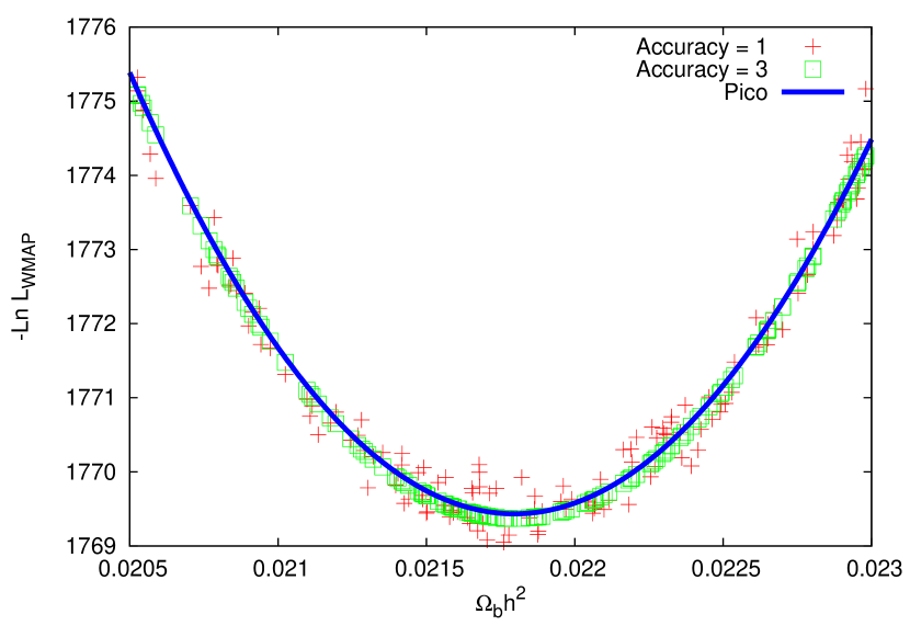
Numerical noise in the power spectrum also leads to noise in the WMAP likelihood as shown in Figure 3. Again, this increases the difficulty in fitting the likelihood with Pico. Just as the power spectrum, this is remedied by running CAMB at higher accuracy. While the level of noise introduced in the likelihood may not be of significant concern when analyzing current CMB data sets, it may represent an important hurdle to overcome for the next generation of experiments. Also evident from Figure 3 is that Pico provides a smooth approximation to the noisy likelihood. This is an important property for algorithms that require differentiating the likelihood such as Hamiltonian Monte Carlo (Hajian, 2007).

Figure 3.— Value of $-\ln L_{\mathrm{WMAP}}$ as a function of $\Omega_{\mathrm{b}}h^{2}$ for a nonflat cosmology. Note that this is near the peak of the likelihood in the full space. The red ($+$) points correspond to the default CAMB accuracies ($1$,$1$,$1$) and the green ($\Box$) points corresponding to using higher accuracy settings ($3$,$3$,$1$). The blue line is the value computed by Pico trained over the $9$ parameter nonflat models discussed in section 3. Note that using the default accuracy in CAMB gives a numerically noisy function, which can lead to variations of $1$ or more log-likelihoods, but Pico gives a smooth function through the high accuracy values.

2.4. Generating the Training Set

As in the first release of Pico, we generate the training set of power spectra and matter transfer function by sampling uniformly from a large box. After training Pico to compute the power spectra, evaluation of the WMAP likelihood, which requires a few seconds, becomes the new bottleneck in parameter estimation. Another significant speed up can be obtained by using Pico to directly fit the likelihood function. However, for the $9$ parameter case we examine in the next section this is a difficult problem. Training Pico over a box in parameter space includes regions that are many thousands of log-likelihoods from the peak and gives a very sparse sampling of the high likelihood region. In practice we are not interested in these areas of parameter space. Instead we aim to compute the likelihood very accurately around the peak of the distribution. This requires generating a training set for Pico that includes only the high likelihood region.

A natural method of accomplishing this is to use the Metropolis Hastings algorithm to find points in the high likelihood region. This can be done efficiently by running CosmoMC Lewis & Bridle (2002) and using Pico to compute the power spectra. To ensure we cover a sufficient volume the chains are run using only the WMAP data and at a higher temperature, meaning the log-likelihood is scaled by a constant factor allowing the chains to explore a larger volume. This step is dominated by the time it takes to run the WMAP likelihood code. Lastly we run the samples through CAMB and the WMAP code to get the true likelihood which will be used to retrain Pico. This step is also quick as it can easily be run in parallel. It is useful to note that this procedure never requires running CAMB in serial making it an ideal application for distributed computing projects such as Cosmology@Home. The training set can be further refined by pruning out data at low likelihood. In the following Pico is trained to compute the likelihood on points within $25$ log-likelihoods of the WMAP peak.

2.5. Polynomial Hierarchy

The process of generating the training set outlined in section 2.4 has the added benefit of giving us a set of power spectra constrained around the peak of the likelihood. We would like to make use of these points by adding them to the power spectra training set. However adding a large weighting of points to a small region of the box will have a negative effet on the accuracy of the algorithm outside this region. Instead we have implemented the ability to use a hierarchy of polynomials with Pico by separately training over the uniformly sampled points in the full box and over only the points in the constrained region. If Pico is given a set of input cosmological parameters within this region it computes the power spectra based on a polynomial fit to this constrained region. For points outside this region, Pico defaults to using the polynomials fit over the full box. While we have found that using only a single set of polynomials trained on the box is sufficient for analysis of current experimental data, this will be a useful feature in the future when data from higher resolution experiments become available.

3. Results

Here we demonstrate the performance of Pico for nonflat cosmologies with the dark energy equation of state, $w_{\mathrm{DE}}$ allowed to vary (but still constant for a given model). In this space Pico fits the power spectrum and likelihood as a function of

$$\left(\Omega_{\mathrm{b}}h^{2},\Omega_{\mathrm{cdm}}h^{2},\Omega_{\mathrm{k}},\theta,\tau,n_{\mathrm{s}},\ln 10^{10}A_{\mathrm{s}},r,w_{\mathrm{DE}}\right).$$

The following sections study the accuracy of Pico in computing the power spectra, matter transfer function, WMAP likelihood as well as its application to parameter estimation based on this $9$ parameter model.

3.1. Power Spectra and Matter Transfer Function

In order to demonstrate Pico’s accuracy and robustness we will test the algorithm for two cases. The first case implements the hierarchy method discussed in section 2.5. Here the training set is divided into two pieces. The first contains $\sim 18000$ samples generated uniformly from the box defined in Table 1, and the second set consists of the $15000$ points constrained to $25$ log-likelihoods from the peak of the WMAP likelihood. For this case the test set consists of $\sim 2000$ points taken from the latter training set. These points were removed from the training set and not used to train Pico.

The models in the training set were run through CAMB at accuracy settings ($3$,$3$,$3$) to compute the true power spectra and transfer functions. As the $\ell$ and $k$ sampling used by CAMB is model dependent it is necessary to spline the power spectra and transfer function so that each is computed at the same $\ell$ or $k$ value. The $\ell$-values were chosen to be those used by CAMB for flat models with lSamp$=3$. For the transfer function we used a unform sampling in $\ln k$. Pico was trained using $6^{\mathrm{th}}$ order polynomials, requiring less than $30$ minutes on a $2.4$GHz desktop.

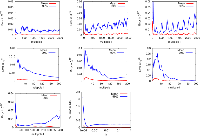
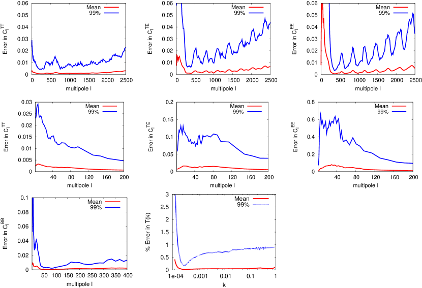
Pico’s performance on this test set is shown in Figure 4. The top $2$ rows show the TT, TE and EE power spectra with the second row focusing on low $\ell$. Results for the BB spectra and matter transfer function are shown in the third row. The two lines in each plot represent the mean error and the error bar that bounds $99\%$ of the test set. For the power spectra the error is plotted in units of the cosmic standard deviation and for the matter transfer function the $y$-axis shows percent error. From the figure we see that over the volume of parameter space important for CMB parameter estimation Pico can compute the power spectra for $99\%$ of models in the training set to better than $4\%$ of cosmic standard deviation, with the mean error around $0.5\%$, over most $\ell$-values. Even the worst fits to the EE power spectra, which occur just after the reionization bump, are only about $25\%$ of the cosmic standard deviation. We also note that many of the models that are fit poorly have very low power in this region so no experiment should be sensitive to these errors. For the transfer function the $99\%$ error bar is around $0.25\%$, and the mean at $0.02\%$, except at very low $k$. This should be sufficient for analysis of data from the next generation of large scale structure experiments.

$0.018$	$<$	$\Omega_{\mathrm{b}}h^{2}$	$<$	$0.034$
$0.06$	$<$	$\Omega_{\mathrm{cdm}}h^{2}$	$<$	$0.2$
$-0.3$	$<$	$\Omega_{\mathrm{k}}$	$<$	$0.3$
$1.02$	$<$	$100\,\theta$	$<$	$1.08$
$0.01$	$<$	$\tau$	$<$	$0.55$
$0.85$	$<$	$n_{\mathrm{s}}$	$<$	$1.25$
$2.75$	$<$	$\ln\left(10^{10}A_{\mathrm{s}}\right)$	$<$	$4.0$
$0$	$<$	$r$	$<$	$2$
$-1.5$	$<$	$w_{\mathrm{DE}}$	$<$	$-0.3$

Table 1Parameter bounds defining the box the training set was sampled from for the example in section 3. This encompasses a volume of at least $3\sigma$ in each parameter around the WMAP maximum likelihood. Note that we also impose the prior that the corresponding Hubble constant for each parameter point lie in the interval $\left[30,100\right]$ which excludes some regions inside the box.

Figure 4.— The above plots compare the performance of Pico with CAMB at high accuracy settings for 9 parameter nonflat models with $w_{\mathrm{DE}}\neq 1$. Pico was trained using the hierarchy method described in section 2.5 and the test set consists of $2000$ points within $25$ log-likelihoods of the WMAP peak. The top two rows show the error compared with CAMB in units of cosmic standard deviation for the TT, TE and EE power spectra at high $\ell$ (top) and low $\ell$ (center). The bottom row shows the error in the BB spectra in units of the cosmic standard deviation and the percent error in the matter transfer function. The two lines on each plot denote the mean error and the error bar that bounds $99\%$ of the test set. We note that much of the error at low $\ell$ in the EE spectra is due to the $1\%$ of models with extremely low power over this range. These spectra are too small to detect even with Planck.

For the second test case the hierarchy method is not used and Pico is only trained on a uniform sample of points from the box in Table 1. For this case the test set consists of a uniform sample of $\sim 2000$ points from the same box. Pico’s performance on this test set is shown in Figure 5. We include this case only to allow comparison with other codes. When Pico is used to explore the parameter posterior based on CMB constraints, which is its main purpose, chains will rarely propose points outside the constrained volume used in the hierarchy method. Therefore Figure 4 provides a better indicator of the types or error incurred by using Pico to compute the power spectra. The regression files on the Pico website implement the hierarchy method.

Figure 5.— The plots are same as those in Figure 4 except here Pico was trained and tested over models sampled uniformly from the box defined by Table 1. Even over this larger region Pico can compute the power spectrum in $99\%$ of the test cases to better than $5\%$ of cosmic standard deviation over most $\ell$ and is never worse than $0.7$ cosmic standard deviation.

3.2. WMAP Likelihood

Next we test the computation of the WMAP likelihood from Pico for two cases. The first uses Pico to compute the power spectrum and then the WMAP code to compute the likelihood and the second uses Pico to directly compute the likelihood. The training set for the likelihood computation consists of $\sim 15000$ points generated using the method described in section 2.4. Another $\sim 2000$ points, generated using the same method, were used as a test set. The absolute error between the likelihood is shown in Figure 6. The plot on the left shows the results of using Pico to compute the power spectrum while the plot on the right shows the results of directly computing the likelihood. For the case of directly evaluating the likelihood, Pico can compute about $90\%$ of the test set better than $0.25$ log-likelihoods. When only using Pico to compute the power spectrum the results are within $0.25$ log-likelihoods for better than $99.5\%$ of the models. The training set and test set were computed using high accuracy CAMB runs and version v2p2p2 of the WMAP likelihood code.

Figure 6.— The plots show the absolute error when evaluating the WMAP likelihood with Pico. In the left plot Pico was used to compute the power spectrum which were fed into the WMAP code. The right plot shows the absolute error when Pico directly evaluates the likelihood. In both cases the likelihood is compared to the value of the WMAP code using high accuracy CAMB power spectra.

3.3. Parameter Estimation

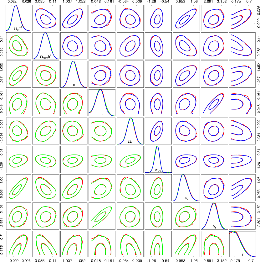
To test the application of Pico to this $9$ parameter model we ran Markov chains using CosmoMC with the WMAP(Hinshaw et al., 2007; Page et al., 2007), ACBAR(Kuo et al., 2004), CBI(Readhead et al., 2004) Boomerang(Montroy et al., 2006; Jones et al., 2006; Piacentini et al., 2006), $2$df(Cole et al., 2005), SDSS (Adelman-McCarthy et al., 2006), and SNLS (Astier et al., 2005) data sets. Chains were run for $3$ cases. The first uses CAMB and the WMAP likelihood code (CAMB$+$WMAP), the second uses Pico to compute the power spectra and transfer function but still uses the official likelihood codes (PICO$+$WMAP) and the third case uses Pico to compute the power spectra, transfer function and the WMAP likelihood (PICO). In third case we did not use Pico to fit the $2$df, SDSS or SNLS likelihood codes. The $1$-dimensional, marginalized posteriors for each of the $9$ parameters are shown along the diagonal in Figure 7. The plots in the lower (upper) triangle in the figure compare the $2$ dimensional posteriors between the PICO$+$WMAP (PICO) case and the CAMB+WMAP case. In all of the plots the CAMB$+$WMAP results are shown in red, the PICO$+$WMAP results in green and the PICO results in red. The lines in the 2D plots denote the $68\%$ and $99\%$ contours. Using $6$ chains run in parallel, the PICO+WMAP chains ran about $60$ times faster than without Pico, requiring about $4$ hours of wall clock time. Using Pico to compute the WMAP likelihood gave another factor of $2.5$ decrease in CPU time giving a total speed up of $\sim 150$ over chains run without Pico. In all cases the chains finished with a Gelman-Rubin statistic less than $1.01$.

Figure 7.— The cosmological parameter posteriors using CAMB and Pico for $9$ parameter nonflat models with $w_{\mathrm{DE}}\neq-1$ based on the WMAP, ACBAR, CBI, Boomerang, SDSS, $2$df and SNLS data sets. The red lines are the result of using CAMB and the WMAP likelihood code. The green lines use Pico to compute the power spectrum but still uses the WMAP likelihood. The blue lines are the result from using Pico to compute the power spectrum and WMAP likelihood. The plots in the lower triangle show the $68\%$ and $99\%$ contours for the chains run using CAMB and PICO with the WMAP likelihood code. The upper triangle compares the CAMB chains to those using Pico to compute the power spectra and WMAP likelihood.

4. Conclusion

This paper describes a major new release of Pico, a fast and accurate code for computing the CMB power spectrum, matter transfer function and the WMAP likelihood. We noted the presence of numerical noise in CAMB at standard accuracy for nonflat models and its effect on the WMAP likelihood. To solve this problem we have generated training sets running CAMB at high accuracy settings. Also we have presented a method of generating a training set that finds the high likelihood region of parameter space without ever running CAMB in serial. This is especially useful for training Pico to fit the WMAP likelihood in large dimensional spaces. Furthermore, Pico can be trained separately on the power spectra in this smaller region of parameter space allowing even more accurate results around the peak of the likelihood while still maintaining the ability to compute the power spectra over a large box in parameter space. The combination of these improvements, along with modifications to the Pico algorithm, have increased its accuracy in computing the power spectrum and likelihood. Also we have extended Pico to compute the power spectrum due to tensor perturbations as well as the matter power spectrum. On the Pico homepage, we provide the new version of Pico and new sets of regression coefficients. We have also released the training code for Pico, allowing users to apply the algorithm to new classes of models and parameter sets. We expect that the accuracy and speed achieved by Pico will be useful for current and future CMB and large scale structure observations. Furthermore, we hope that the concept, embodied by Pico, of exploiting massively parallel computing resources to solve inherently serial numerical problems will find applications beyond the immediate domain of cosmological parameter estimation.

References

- Adelman-McCarthy et al. (2006) J. K. Adelman-McCarthy et al. [SDSS Collaboration], Astrophys. J. Suppl. 162, 38 (2006)
- Astier et al. (2005) P. Astier et al. [The SNLS Collaboration], Astron. Astrophys. 447, 31 (2006)
- Auld et al. (2006) T. Auld, M. Bridges, M. P. Hobson and S. F. Gull, Mon. Not. Roy. Astron. Soc. Lett. 376, L11 (2007)
- Auld et al. (2007) T. Auld, M. Bridges and M. P. Hobson, arXiv:astro-ph/0703445.
- Catlett et al. (2007) C. Catlett et al., HPC and Grids in Action, Ed. Lucio Grandinetti, IOS Press ’Advances in Parallel Computing’ series, Amsterdam (2007)
- Cole et al. (2005) S. Cole et al. [The 2dFGRS Collaboration], Mon. Not. Roy. Astron. Soc. 362, 505 (2005)
- Fendt & Wandelt (2007) W. A. Fendt and B. D. Wandelt, Astrophys. J. 654, 2 (2007)
- Habib et al. (2007) S. Habib, K. Heitmann, D. Higdon, C. Nakhleh and B. Williams, arXiv:astro-ph/0702348.
- Hajian (2007) A. Hajian, Phys. Rev. D 75, 083525 (2007)
- Heitmann et al. (2006) K. Heitmann, D. Higdon, C. Nakhleh and S. Habib, Astrophys. J. 646, L1 (2006)
- Hinshaw et al. (2007) G. Hinshaw et al. [WMAP Collaboration], Astrophys. J. Suppl. 170, 288 (2007)
- Jimenez et al. (2004) R. Jimenez, L. Verde, H. Peiris and A. Kosowsky, Phys. Rev. D 70, 023005 (2004)
- Kaplinghat et al. (2002) M. Kaplinghat, L. Knox and C. Skordis, Astrophys. J. 578, 665 (2002)
- Karhunen (1946) Karhunen, K., Ann, Acad. Sci. Fennicae, 37 (1946)
- Kirby (2001) Kirby, M. 2001, Geometric Data Analysis: An Empirical Approach to Dimensionality Reduction and the Study of Patterns (New York: John Wiley & Sons)
- Kuo et al. (2004) C. l. Kuo et al. [ACBAR collaboration], Astrophys. J. 600, 32 (2004)
- Jones et al. (2006) W. C. Jones et al., Astrophys. J. 647, 823 (2006)
- Lewis et al. (2000) A. Lewis, A. Challinor and A. Lasenby, Astrophys. J. 538, 473 (2000)
- Lewis & Bridle (2002) A. Lewis and S. Bridle, Phys. Rev. D 66, 103511 (2002)
- Loève (1955) Loève, M. 1955, Probability Theory (Princeton: Van Nostrand)
- MacQueen (1967) MacQueen, J. 1967, Proc. 5th Berkeley Symp. on Mathematical Statistics and Probability, 1, 281
- Montroy et al. (2006) T. E. Montroy et al., Astrophys. J. 647, 813 (2006) [arXiv:astro-ph/0507514].
- Page et al. (2007) L. Page et al. [WMAP Collaboration], Astrophys. J. Suppl. 170, 335 (2007)
- Piacentini et al. (2006) F. Piacentini et al., Astrophys. J. 647, 833 (2006) [arXiv:astro-ph/0507507].
- Readhead et al. (2004) A. C. S. Readhead et al., Astrophys. J. 609, 498 (2004) [arXiv:astro-ph/0402359].
- Sandvik et al. (2004) H. B. Sandvik, M. Tegmark, X. M. Wang and M. Zaldarriaga, Phys. Rev. D 69, 063005 (2004)
- Seljak & Zaldarriaga (1996) U. Seljak and M. Zaldarriaga, Astrophys. J. 469, 437 (1996)
- Spergel et al. (2007) D. N. Spergel et al. [WMAP Collaboration], Astrophys. J. Suppl. 170, 377 (2007)
- Tegmark & Bunn (1995) M. Tegmark and E. F. Bunn, Astrophys. J. 455, 1 (1995)