Black hole formation and slow-roll inflation

Abstract

Black hole formation may occur if the spectrum of the curvature perturbation $\zeta$ increases strongly as the scale decreases. As no such increase is observed on cosmological scales, black hole formation requires strongly positive running $n^{\prime}$ of the spectral index $n$, though the running might only kick in below the ‘cosmological scales’ probed by the CMB anisotropy and galaxy surveys. A concrete and well–motivated way of producing this running is through the running mass model of slow roll inflation. We obtain a new observational bound $n^{\prime}<0.026$ on the running provided by this model, improving an earlier result by a factor two. We also discuss black hole production in more general scenarios. We show that the usual conditions $\epsilon\ll 1$ and $|\eta|\ll 1$ are enough to derive the spectrum ${\cal P}_{\zeta}(k)$, the introduction of higher order parameters $\xi^{2}$ etc. being optional.

I Introduction

The primordial curvature perturbation $\zeta$ is only of order $10^{-4}$ on cosmological scales, but it might be of order 1 on smaller scales. Primordial black holes will then form as those scales enter the horizon, with possibly observable consequences. The purpose of this paper is to see to what extent the value of order 1 is reasonable, taking into account observational constraints and current thinking about the origin of $\zeta$.

In Section II we see what is required for black hole formation, in terms of the spectral index $n(\ln k)\equiv d\ln{{\cal P}_{\zeta}}/d\ln k$, which specifies the scale-dependence of the spectrum of $\zeta$. Averaged over the whole range of scales we need strongly increasing $n$ corresponding to running $n^{\prime}\sim 10^{-2}$. Up to this point we assumed nothing about the origin of $\zeta$. In Section III we introduce the assumption that it originates from the inflaton perturbation during slow-roll inflation (the standard paradigm). Within this paradigm, the only extant model giving the required running $n^{\prime}$ is the running mass model, which typically makes $n^{\prime}$ roughly constant hence requiring $n^{\prime}\sim 10^{-2}$ on cosmological scales.

In Section IV we ask whether such a large value of the running is still permitted by current data, thereby updating an earlier work. We find that it is.

The question then arises, whether black hole formation can still be achieved if $n^{\prime}$ is negligible on cosmological scales, as might be required by future data. In Sections V to VIII we show that black hole formation can indeed be achieved within the standard paradigm. Along the way, we are led to consider the standard paradigm in more detail than before.

In Section IX we depart from the standard paradigm, by allowing a curvaton-type mechanism to contribute to the curvature perturbation. We show that black hole formation can occur if there is a switch from the standard paradigm to a curvaton-type paradigm as we go up in scale, or vice-versa. We conclude in Section X.

II Forming black holes

II.1 Viable black hole formation

The curvature perturbation $\zeta$ is time-independent during any era when there is a unique relation $P(\rho)$ between pressure and energy density lms . From the success of the BBN calculation, we know that such is the case to high accuracy a few Hubble times before cosmological scales start to come inside the horizon. On cosmological scales, the spectrum ${{\cal P}_{\zeta}}(k)$ is then observed to be about $(5\times 10^{-5})^{2}$ spergel .

When smaller scales start to come inside the horizon ${{\cal P}_{\zeta}}(k)$ could be bigger. To discuss that case, recall that the typical value of $\zeta({\mathbf{x}})$ in the observable Universe mybox , smoothed on the scale $k^{-1}$, is of order ${{\cal P}_{\zeta}}^{1/2}(k)$. If ${{\cal P}_{\zeta}}^{1/2}(k)$ is bigger than $10^{-2}$ or so, then black holes will form BBN with an abundance that can be ruled out ruleout by a variety of observations. A somewhat smaller value, say ${{\cal P}_{\zeta}}^{1/2}\sim 10^{-3}$, would give an abundance whose effect may be observable in the future. We want to see how such a value may be generated over some range of $k$.

The spectral index $n$ is defined by

$$n(k)-1=\frac{d\ln{{\cal P}_{\zeta}}(k)}{d\ln k}\simeq-\frac{d\ln{{\cal P}_{\zeta}}(N)}{dN}.$$ (1)

In the final expression we assume almost-exponential inflation, with $N(k)$ the number of $e$-folds of inflation remaining after the epoch of horizon exit $k=aH$ for the scale $k$. We will freely use $N$ as an alternative variable to $\ln k$.

We take $N_{0}=50$ unless otherwise stated, where the subscript 0 denotes the epoch of horizon exit for the present Hubble scale $k=H_{0}$. This is the largest observable scale, and smaller scales leave the horizon $\Delta N>0$ $e$-folds later. For scales probed by WMAP and galaxy surveys, $\Delta N\leq 7$ spergel .

Until Section IXB we will assume that the black holes form on the scale leaving the horizon at the end of inflation, corresponding to $N=0$. We will take the criterion for significant black hole formation to be ${{\cal P}_{\zeta}}(0)=10^{-3}$. Then we need $\ln[{{\cal P}_{\zeta}}(0)/{{\cal P}_{\zeta}}(N_{0})]\simeq\ln(10^{-3}/10^{-9})\simeq 14$. With constant $n$ this requires $n-1\simeq 14/N_{0}\simeq 0.3$. This was compatible with observation for many years but is now excluded.

Taking instead $n^{\prime}\equiv dn/d\ln k$ to be constant black hole formation requires

$$14=\ln\left[\frac{{{\cal P}_{\zeta}}(0)}{{{\cal P}_{\zeta}}(N_{0})}\right]=N_{0}(n_{0}-1)+\frac{1}{2}N_{0}^{2}n^{\prime}.$$ (2)

Since observation requires $n_{0}-1\simeq-0.05$ spergel , the first term is negligible and we need $n^{\prime}\simeq 28/N_{0}^{2}\simeq 0.01$. As we will see, this is compatible with observation. At the end of inflation, $n_{\rm end}-1\simeq n^{\prime}\times N_{0}\sim 0.5$. This might be regarded as more or less compatible with the requirement $|n-1|\ll 1$, that must hold if $\zeta$ at the end of inflation is generated by the perturbation in a single light field ss ; treview ; mycurv . We are going to assume such a scenario and therefore rule out $|n_{\rm end}-1|\gtrsim 1$.

Finally, suppose that $n^{\prime}$ increases monotonically as we go down in scale. A significant increase would require $|n_{\rm end}-1|\gtrsim 1$ which we rule out. A significant decrease would require $n^{\prime}_{0}$ significantly bigger than $0.01$, which as we will see would be in conflict with observation.

II.2 The case ${{\cal P}_{\zeta}}\gg 1$

We end this section by discussing briefly the case ${\cal P}_{\zeta}(k)\gg 1$. If $\zeta$ is generated from the inflaton perturbation during slow-roll inflation (the standard paradigm), this is ruled out. The reason is that the regime ${{\cal P}_{\zeta}}\gtrsim 1$ then corresponds to eternal inflation eternal , whose duration is indefinitely long. Then the slow roll model has nothing to do with the observed perturbations, which instead have to be generated when the eternal inflation is over.

However, such a perturbation could also be generated by the perturbation of a curvaton-like field curvaton ; mycurv , as one can readily understand from the non-perturbative formula lms ; deltan ; ss $\zeta=\delta N$ which makes sense no matter how big is $\zeta$. In that case, a local observer would notice nothing amiss before horizon entry, and it is not clear what will happen at horizon entry.

III Running mass model

Now we assume that $\zeta$ is generated by the inflaton perturbation in a single-field slow-roll model. Of the many such models that have been proposed, the only one giving the large positive running required for black hole formation is the running mass model running ; r2 ; r3 ; r4 ; lgl . This model invokes softly broken global supersymmetry during inflation, with a potential

$$V=V_{0}\pm\frac{1}{2}m^{2}(\phi)\phi^{2},$$ (3)

and a running mass $m^{2}(\phi)$ whose form is determined by Renormalization Group Equations (RGE’s).

Over the limited range of cosmological scales, $n(N)$ typically has the two-parameter form

$$\frac{n(N)-1}{2}=se^{c(N_{0}-N)}-c.$$ (4)

With

$$c\simeq 10^{-1}\quad{\rm to}\quad 10^{-2}$$ (5)

this gives

$$n_{0}=2(s-c)-1,\qquad n_{0}^{\prime}=2sc,$$ (6)

whose inverse is

$$c=-\frac{n_{0}-1}{4}\pm\sqrt{\left(\frac{n_{0}-1}{4}\right)^{2}+\frac{n_{0}^{\prime}}{2}}.$$ (7)

We see that significant negative running is forbidden;

$$n_{0}^{\prime}>-(n_{0}-1)^{2}/8\sim-3\times 10^{-4}.$$ (8)

Higher derivatives $n^{(m)}\equiv d^{m}n/d(-N)^{m}$ are suppressed;

$$n^{(m+1)}\simeq cn^{(m)},\qquad m\geq 1,$$ (9)

but as the form (4) is only approximate one should not take higher derivatives too seriously.

Going further down in scale, the form of $n(N)$ depends on the assumed interactions that determine the RGE’s. Typically, $n^{\prime}$ will increase or decrease monotonically. As we have seen, black hole formation will then need $n^{\prime}$ to have a roughly constant value, $n^{\prime}\sim 10^{-2}$, and this can be achieved with suitable interactions lgl . From Eq. (7), $n^{\prime}\sim 10^{-2}$ corresponds to to $c\simeq s\simeq\pm\sqrt{n_{0}^{\prime}/2}$, making $|c|\sim 10^{-1}$, in agreement with the expectation (5).

IV Observational bound on the running mass model

The most recent comparison of the running mass model with observation was made in 2004 using WMAP (year on) and galaxy survey data available at the time r4 . It gave $n_{0}^{\prime}<0.04$ or so, easily allowing black hole formation in versions of the model where $n^{\prime}$ does not increase too strongly going down in scale. In this section we report an update to the earlier bound, using year three WMAP data and more recent galaxy survey results.

In the earlier fit, we took $c$ and $s$ as the parameters to be fitted, and only afterward generated contour plots of $n_{0}$ versus $n^{\prime}_{0}$. In the present fit, we instead took $n_{0}$ and $n^{\prime}_{0}$ as the parameters to be fitted. Taking advantage of the fact that Eq. (4) practically excludes negative $n_{0}^{\prime}$, and that it requires $n^{\prime}$ to have slow variation, we took $n^{\prime}$ to be constant and imposed $n_{0}^{\prime}>0$ as a prior. As in the previous fit we took the tensor perturbation to be negligible since that is a prediction of the model. This differs substantially from the method adopted in spergel where the running of the spectral index was let free to negative values and where tensors were included. In that case a negative value of the running is obtained, with no running excluded at the level of $\sim 1\sigma$ (see e.g. spergel ; kkmr ; easther ; finelli ; ringe ). While this approach is obviously correct when a general set of inflationary models is considered, it is important to stress that in our case, where we don’t consider models with $n^{\prime}<0$, the inclusion of those models could bias the result towards more restrictive bounds. Moreover, a model with $n^{\prime}=0$ gives an acceptable goodness-of-fit to the WMAP data and it is therefore statistically legitimate to assume the prior $n^{\prime}\geq 0$.

As is now common practice, we base our analysis on Markov Chain Monte Carlo methods making use of the publicly available cosmomc package Lewis:2002ah . We sample the following dimensional set of cosmological parameters, adopting flat priors on them: the physical baryon and CDM densities, $\omega_{b}=\Omega_{b}h^{2}$ and $\omega_{c}=\Omega_{c}h^{2}$, the ratio of the sound horizon to the angular diameter distance at decoupling, $\theta_{s}$, the scalar spectral index, $n$, and the optical depth to reionization, $\tau$. We consider purely adiabatic initial conditions. We choose a pivot scale at $k=0.002h^{-1}$Mpc.

The MCMC convergence diagnostics are done on $7$ chains applying the Gelman and Rubin “variance of chain mean”$/$“mean of chain variances” $R$ statistic for each parameter. Our $1-D$ and $2-D$ constraints are obtained after marginalization over the remaining “nuisance” parameters, again using the programs included in the cosmomc package. Temperature, cross polarization and polarization CMB fluctuations from the WMAP 3 year data spergel ; Page:2006hz ; Hinshaw:2006ia ; Jarosik:2006ib are considered and we include a top-hat age prior $10\mathrm{\ Gyr}<t_{0}<20\mathrm{\ Gyr}$.

We also consider the small-scale CMB measurements of the CBI 2004ApJ…609..498R , VSA 2004MNRAS.353..732D , ACBAR 2002AAS…20114004K and BOOMERANG-2k2 2005astro.ph..7503M experiments. We combine the CMB data with the real-space power spectrum of galaxies from the 2dF survey 2005MNRAS.362..505C . We restrict the analysis to a range of scales over which the fluctuations are assumed to be in the linear regime (technically, $k<0.2h^{-1}$ Mpc) and we marginalize over a bias $b$ considered as an additional nuisance parameter.

Figure 1: $68\%$ and $95\%$ c.l. likelihoods in the $n-n^{\prime}$ plane from the WMAP data alone (Top Panel) and WMAP+LSS (Bottom Panel).

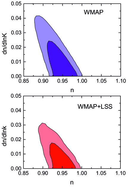
In Figure 1 we plot the $68\%$ and $98\%$ confidence levels in the $n$-$n^{\prime}$ plane for two different choices of our datasets: WMAP data alone, that should be considered as the most conservative result, and “WMAP+LSS” that includes the remaining CMB data and galaxy clustering data from 2dF.

As we can see from the Figure, when negative running is not considered, the data is still in good agreement with a small, but still non-zero running. When the WMAP dataset is considered we found a $95\%$ c.l. upper limit of $n^{\prime}<0.039$, while the spectral index is bound to be $n=0.935_{-0.049}^{+0.039}$ again at $95\%$. The best fit (maximum likelihood) model has a negligible running $n^{\prime}=0.005$ and $n=0.953$. When the remaining cosmological data are included, we found a stronger bound on running, with $n^{\prime}<0.026$, and $n=0.940_{-0.040}^{+0.032}$ at $95\%$ c.l.. The best fit (maximum likelihood) model has parameters $n^{\prime}=0.0026$ and $n=0.951$. We conclude that the value $n^{\prime}\sim 10^{-2}$ required by the running mass model is still viable.

We have checked that our limits on n’ are also consistent with the WMAP results even in the case when a negative running is allowed. The fitted parametes are in reasonable agreement with the limits we quoted above, even if slightly more stringent due to the inclusion of negative running.

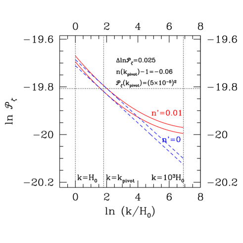
In performing this fit, we chose a pivot point $k=0.002h\,\mbox{Mpc}^{-1}$, corresponding to $\Delta N=1.8$. Our fitted value $n=0.94$ therefore corresponds to $n_{0}=0.94-1.8n^{\prime}$. (Recall that the subscript 0 denotes the scale $k=H_{0}=0.00033h\,\mbox{Mpc}^{-1}$.) In Figure 2, we plot the shape of the spectrum with (i) no running and $n=0.95$, (ii), $n^{\prime}=0.01$, and $n=0.95$ at the pivot point. In the second case, $n-1$ soon climbs to positive values as we go down below the pivot scale. (The finite width of the band is not important at this stage, and will be discussed in Section VI.)

Figure 2: The band corresponds to the spectrum ${{\cal P}_{\zeta}}$ versus $\ln k$, with constant slope corresponding to $n=0.94$. The width of the band corresponds to a fractional uncertainty $0.025$. The range of $\ln k$ corresponds to the range of cosmological scales, explored by observation of the cmb anisotropy and galaxy surveys. We see that the band is narrow enough to make the variation of ${{\cal P}_{\zeta}}$ significant over the cosmological range.

V Slow roll formalism

In the future, observation may require negligible running on cosmological scales. We have seen that this would not permit black hole formation if $n^{\prime}$ increased or decreased monotonically as we go down in scale, but black hole formation may still be possible with a more complicated behavior of $n^{\prime}$. We are going to exhibit a couple of forms of $n(k)$ that would do the job, and still be compatible with slow-roll inflation. In order to do that, we need to consider carefully what the slow-roll approximation involves. 

The slow roll formalism is reviewed for instance in treview ; book ; al ; paris . It starts from the exact Friedmann equation

$$3M_{\rm P}^{2}H^{2}=V(\phi)+\frac{1}{2}\dot{\phi}^{2},$$ (10)

and the exact unperturbed field equation

$$\ddot{\phi}+3H\dot{\phi}+\frac{dV}{d\phi}=0,$$ (11)

from which follow the identity

$$\dot{H}M_{\rm p}^{2}=-\dot{\phi}^{2}/2.$$ (12)

In its most basic form, the slow-roll approximation consists of the two assumptions;

$$\left|\frac{\dot{\phi}^{2}}{H^{2}M_{\rm p}^{2}}\right|\ll 1\qquad\left|\frac{\ddot{\phi}}{H\dot{\phi}}\right|\ll 1.$$ (13)

These assumptions are usually stated in the equivalent forms

$$3M_{\rm P}^{2}H^{2} \simeq V(\phi)$$ (14)

$$3H\dot{\phi} \simeq -V^{\prime}(\phi),$$ (15)

and they imply $\epsilon\ll 1$ where

$$\epsilon\equiv\frac{1}{2}M_{\rm P}^{2}\left(\frac{V^{\prime}}{V}\right)^{2}.$$ (16)

To calculate the spectrum ${{\cal P}_{\zeta}}(k)$ one usually considers additional parameters;

$$\eta \equiv M_{\rm P}^{2}\frac{V^{\prime\prime}}{V}$$ (17)

$$\xi^{2} \equiv M_{\rm P}^{4}\frac{V^{\prime}V^{\prime\prime\prime}}{V^{2}}$$ (18)

$$\sigma^{3} \equiv M_{\rm P}^{6}\frac{V^{\prime 2}V^{\prime\prime\prime\prime}}{V^{3}}.$$ (19)

The last two parameters can have either sign despite the notation.

Using Eq. (15) one finds

$$\frac{d\ln H}{dN} = \epsilon$$ (20)

$$\frac{d(\ln\epsilon)}{dN} = -4\epsilon+2\eta$$ (21)

$$\frac{d\eta}{dN} = -2\epsilon\eta+\xi^{2}$$ (22)

$$\frac{d\xi^{2}}{dN} = -(4\epsilon-\eta)\xi^{2}+\sigma^{3}.$$ (23)

More generally one can define

$$\alpha_{m}\equiv M_{\rm P}^{2m}\frac{V^{\prime m-1}(d^{m+1}V/d\phi^{m+1})}{V^{m}},$$ (24)

which satisfy

$$\frac{d\alpha_{m}}{dN}=\left[(m-1)\eta-2m\epsilon\right]\alpha_{m}+\alpha_{m+1},$$ (25)

Assuming that the first derivative of Eq. (15) is also a valid approximation, one finds

$$\frac{\ddot{\phi}}{H\dot{\phi}}=\epsilon-\eta,$$ (26)

Comparing Eq. (15) with the exact equation, we see that the fractional error in Eq. (15) is ${\cal O}(\epsilon,\eta)$, and so we require the additional condition

$$|\eta|\ll 1.$$ (27)

Assuming that the curvature perturbation is generated from the vacuum fluctuation of $\delta\phi$, its spectrum in the slow roll approximation is given by spec

$${{\cal P}_{\zeta}}(k) = \frac{1}{24\pi^{2}M_{\rm P}^{4}}\frac{V}{\epsilon}\left[1+{\cal O}\left(\epsilon,\eta\right)\right],$$ (28)

$$= \frac{1}{12\pi^{2}M_{\rm p}^{6}}\frac{V^{3}}{\left(3H\dot{\phi}\right)^{2}}\left[1+{\cal O}(\epsilon,\eta)\right]$$ (29)

The right hand side is evaluated at the epoch of horizon exit. The displayed uncertainty takes account of the fractional error in the slow roll approximation that we just estimated, and first order (linear) corrections to the calculation of the vacuum fluctuation described by the Mukhanov-Sasaki equation ms ; ls ; gs ; ewanbeyond (It does not account for nonlinear effects, coming from interactions of $\delta\phi$. Such effects, which would generated non-gaussianity of $\zeta$, are expected to be small maldacena .

Now differentiate Eq. (28) with respect to $\ln k$, using $d\ln k=-dN$ and ignoring the uncertainty. One finds specind

$$n-1 = 2\eta-6\epsilon$$ (30)

$$n^{\prime} = 2\xi^{2}+24\epsilon^{2}-16\epsilon\eta.$$ (31)

The error in $n-1$, coming from the derivative of the error in ${{\cal P}_{\zeta}}$, is ${\cal O}(\xi^{2},\epsilon^{2},\epsilon\eta)$. We will assume that there is no cancellation between the two terms of Eq. (30), and make a similar assumption for $n^{\prime}$ and higher derivatives. Also, we will assume that $\epsilon$ is negligible compared with $\eta$, $\xi^{2}$ and any other relevant $\alpha_{m}$. Then the fractional uncertainty in $n-1$ will be small if and only if

$$|\xi^{2}|\ll|\eta|.$$ (32)

Similarly, the fractional error in $n^{\prime}$ will be small if and only if

$$|\sigma^{3}|\ll|\xi^{2}|.$$ (33)

In principle one can go on to calculate higher derivatives of $n$, requiring a more extended hierarchy

$$|\alpha_{m+1}|\ll|\alpha_{m}|.$$ (34)

From Eq. (21), this is equivalent to

$$\left|\frac{d^{m}{\ln\epsilon}}{dN^{m}}\right|\ll\left|\frac{d^{m-1}{\ln\epsilon}}{dN^{m-1}}\right|.$$ (35)

We have been exploring the validity of successive derivatives with respect to $N$, of the slow-roll approximation Eq. (30) for $n-1$. Barring cancellations, the validity of these up to a given order will be equivalent to the validity of derivatives of the slow-roll approximation for the field equation Eq. (11), up to one higher order. To see this, start with Eq. (26) which expresses the validity of the first derivative of Eq. (11). Put it into Eq. (11), and use $\ln(1+x)\simeq x$ to find the approximation

$$\ln(|V^{\prime}|)=\ln(3H|\dot{\phi}|)+\frac{\epsilon-\eta}{3}.$$ (36)

Assuming that the derivative of the approximation Eq. (26) is also valid, we can differentiate this with respect to $N$:

$$\frac{d\ln|V^{\prime}|}{dN}=\frac{d\ln(3H\dot{\phi})}{dN}+\frac{d}{dN}\left(\frac{\epsilon-\eta}{3}\right).$$ (37)

Barring cancellations, the first term on the right hand side is of order $n-1$ as is easily seen by comparing it with the derivative of Eq.(29). Therefore, barring cancellations, the validity of this approximation is indeed equivalent to the validity of the first derivative of the approximation Eq. (30), and so on for higher derivatives.

The equivalence that we saw in the last paragraph means that the standard slow-roll approximation for $n-1$, $n^{\prime}$ and so on will be valid, if the second, third and so on derivatives of the slow-roll approximation Eq. (26) to the exact field equation Eq. (11) are valid. Reverting to our assumption that $\epsilon$ is negligible, we conclude that the hierarchy Eq. (32), Eq. (33) etc. will hold (justifying the standard formulas for $n-1$, $n^{\prime}$ etc.) to the extent that derivatives of the slow-roll approximation Eq. (26) hold.

With the hierarchy in place, one can systematically improve the predictions (28), (30) and (31) ls ; gs . The hierarchy is in general satisfied by the running mass model, and including the leading order correction ls , the running mass prediction (4) becomes r3

$$\frac{n(N)-1}{2} = \left(s+1.06cs\right)e^{c(N_{0}-N)}-c$$ (38)

$$\simeq \left(s+0.50n^{\prime}\right)e^{c(N_{0}-N)}-c.$$ (39)

Such corrections are usually equivalent to a change in parameters whose values are not known (in this case, a change to $s$), making them of limited practical importance.

Of course, a given inequality in the hierarchy will fail for a few Hubble times if its right hand side passes through zero. For instance, Eq. (32) will fail if $\eta$ passes through zero. Then, if $\epsilon$ is negligible, $n-1$ will pass through zero as well, and while it is doing so the fractional error in its predicted value will become large. According to our fit to the data, $n(N)-1$ will indeed pass through zero on some scale near the bottom end of the cosmologically accessible range, if $n^{\prime}$ has a slowly varying value of order $10^{-2}$. The passage of $n-1$ through zero need not be a matter of concern, as the absolute error remains the same. The running mass prediction (39) should remain valid even as $n$ passes through zero.

More generally, it could happen that derivatives of Eq. (15) beyond the first are invalid over an extended range, so that the hierarchy fails over an extended range. To handle such cases one can use the exact (at first order) Mukhanov-Sasaki equation or an analytic approximation ewanbeyond .

VI Finite difference version of the spectral index

Although the hierarchy leads to simple and widely-used results, we have seen that its use may sometimes be problematic and we will see some more examples of that in the following two sections. For that reason, we explain in this section how the hierarchy can if necessary be avoided.

The starting point is to realise that the prediction Eq. (28), with a suitably small error, will accurately define the variation of ${{\cal P}_{\zeta}}$ over a finite range, even if the mathematical derivative should have large errors (coming for instance from an oscillation or a break). This is illustrated in Figure 2.

Let us therefore redefine $n-1$ so that it specifies a finite difference:

$$\tilde{n}-1\equiv\frac{\ln{\cal P}_{\zeta 2}-\ln{\cal P}_{\zeta 1}}{\Delta\ln k},$$ (40)

where $\Delta\ln k\equiv\ln k_{2}-\ln k_{1}$ and ${\cal P}_{\zeta i}\equiv{{\cal P}_{\zeta}}(k_{i})$. To the extent that observational bounds on the variation of $n(k)$ are quite weak, this finite difference is really about all that observation can determine at present, with $\Delta\ln k\simeq 7$ or so.

The error in $\tilde{n}-1$ generated by a fractional error $x$ in the prediction (28) will be at most of order

$$\delta(\tilde{n}-1)\simeq\frac{x}{\Delta\ln k}.$$ (41)

Let us assume $x\simeq 0.025$, corresponding to Eq. (28) with $\epsilon\ll|\eta|\simeq 0.05$ (the observed value of $|n-1|$). Then the error in the theoretical prediction will be small, if the prediction satisfies

$$|\tilde{n}-1|\gg\frac{x}{\Delta\ln k}\simeq 0.004.$$ (42)

As illustrated in Figure 2, this is very well satisfied if $\tilde{n}-1$ has the observed value $\simeq-0.05$.

We can go a bit further, to consider a finite-difference version of the running;

$$\tilde{n}^{\prime} \equiv \left(\frac{\ln{\cal P}_{\zeta 1}-\ln{\cal P}_{\zeta 3}}{\Delta\ln k/2}-\frac{\ln{\cal P}_{\zeta 3}-\ln{\cal P}_{\zeta 2}}{\Delta\ln k/2}\right)/\left(\Delta\ln k/2\right)$$ (43)

$$= \left(\frac{\ln{\cal P}_{\zeta 2}-2\ln{\cal P}_{\zeta 3}+\ln{\cal P}_{\zeta 1}}{(\Delta\ln k)^{2}/4}\right),$$ (44)

with $2\ln k_{3}\equiv\ln k_{1}+\ln k_{2}$. The error in $\tilde{n}^{\prime}$ generated by the error $x$ in the prediction will be at most of order

$$\delta\tilde{n}^{\prime}\sim\frac{10x}{(\Delta\ln k)^{2}}.$$ (45)

The error will be small if the prediction satisfies

$$|\tilde{n}^{\prime}|\gg\frac{10x}{(\Delta\ln k)^{2}}\simeq 5\times 10^{-3},$$ (46)

where we again set $x=0.025$ as an illustration. Taking account of the uncertainties, the prediction for the finite-difference version of the running may be valid if $n^{\prime}\sim 10^{-2}$.

VII Flow equations

In the above analysis we worked directly with the potential. A different approach works initially with the field $\phi(t)$, connecting only later with the potential. The starting point is Eq. (12), providing a parameter $\epsilon_{H}$ which may be written in various forms;

$$\epsilon_{H} \equiv -\frac{\dot{H}}{H^{2}}=\frac{d(\ln H)}{dN}$$ (47)

$$= \frac{1}{2M_{\rm P}^{2}}\left(\frac{d\phi}{dN}\right)^{2}=2M_{\rm P}^{2}\left(\frac{1}{H}\frac{dH}{d\phi}\right)^{2},.$$

Its derivatives satisfy the exact set of equations

$$\frac{d(\ln\epsilon_{H})}{dN} = -2(\epsilon_{H}+\delta_{1})$$ (48)

$$\frac{d\delta_{m}}{dN} = (\delta_{1}-m\epsilon_{H})\delta_{m}+\delta_{m+1},$$ (49)

where gs ; ewanbeyond

$$\delta_{m}\equiv d^{m}\phi/dt^{m}/H^{m}\dot{\phi}.$$ (50)

Equivalently, one can use $\phi$ instead of $N$ as the variable. Then flow1

$$\frac{d(\ln(\epsilon_{H})}{d\phi} = -2(\epsilon_{H}-\beta_{1})$$ (51)

$$\frac{d\beta_{m}}{d\phi} = \left[(m-1)\beta_{1}-m\epsilon_{H}\right]\beta_{m}+\beta_{m+1},$$ (52)

where flow2

$$\beta_{m}\equiv\left(\frac{2M_{\rm P}}{H}\right)^{m}\left(\frac{dH}{d\phi}\right)^{m-1}\frac{d^{m+1}H}{d\phi^{m+1}},$$ (53)

These are referred to as flow equations.

The flow equations (equivalently Eqs. (49) and (50)) resemble Eqs. (20), (21), and (25) but are exact. Slow roll with the potential hierarchy (34), up to $m=M$, is obtained if there is a hierarchy

$$|\delta_{m+1}|\ll|\delta_{m}|,$$ (54)

or equivalently

$$|\beta_{m+1}|\ll|\beta_{m}|$$ (55)

up to $m=M+1$. Following flow2 one might call this the ‘Hubble hierarchy’, as opposed to the ‘potential hierarchy’ (34).

Conversely, if the potential hierarchy is satisfied up to $m=M$, then one can expect the solution $\phi(t)$ to satisfy the hierarchy (55) (equivalently (54)) up to $m=M+1$, at least for low $M$. This is because the slow-roll approximation (15) is known to be a strong attractor for a wide range of initial conditions. As with the potential hierarchy, the Hubble hierarchy will fail briefly if a parameter ($\delta_{m}$ or $\beta_{m}$ passes through zero, and it might not be valid at all.

VIII Two forms for the potential

Now we consider forms of the potential, which would permit slow roll inflation leading to black hole formation, and be consistent with a negligible value of $n_{0}^{\prime}$. A common procedure for generating potentials consistent with assigned values of (say) $n_{0}$ and $n_{0}^{\prime}$ uses the flow equations. The equations are numerically integrated with an initial hierarchy imposed such as $|\beta_{m+1}|/|\beta_{m}|<1/5$ ce or $1/10$ flow1 . This procedure is quite complicated, and will obviously miss potentials violating the initial hierarchy as discussed at the end of the previous section.

Our procedure will be to simply specify suitable forms for $d(\ln\epsilon)/dN)$. (It resembles the one advocated in andrewflow .) From these the potential can be constructed using

$$\epsilon(N) = \epsilon(N_{0})\exp\left[-\int^{N_{0}}_{N}\frac{d\ln\epsilon}{dN}\right]$$ (56)

$$H(N) = H(N_{0})\exp\left[-\int^{N_{0}}_{N}\epsilon(N)dN\right]$$ (57)

$$\phi(N_{0})-\phi(N) = M_{\rm P}\int^{N_{0}}_{N}\sqrt{2\epsilon(N)}dN$$ (58)

$$V(\phi) = 3M_{\rm P}^{2}H^{2}(\phi).$$ (59)

The value $H(N_{0})$ is determined once the inflation scale $V(N_{0})$ is set, and then $\epsilon(N_{0})$ is obtained from Eq. (28) using the observed value ${{\cal P}_{\zeta}}(N_{0})=(5\times 10^{-5})^{2}$.

To keep things simple we focus on small-field inflation, which corresponds to $\epsilon$ far below 1. To be precise, we assume $\epsilon\ll 1/N_{0}$ for $0<N<N_{0}$, corresponding to tensor fraction $r\ll 16/N_{0}\simeq 0.03$. Then $V$ can be taken to be constant, and black hole formation requires

$$\Delta\ln\epsilon\equiv\ln[\epsilon(N_{0})/\epsilon(0)]\simeq\ln[{{\cal P}_{\zeta}}(0)/{{\cal P}_{\zeta}}(N_{0})]\simeq 14.$$ (60)

The predictions for the spectral index and its running are then

$$\frac{n-1}{2} = \eta\equiv M_{\rm P}^{2}\frac{V^{\prime\prime}}{V}~{}\left(\simeq\frac{1}{2}\frac{d\ln\epsilon}{dN}\right)$$ (61)

$$\frac{n^{\prime}}{2} = \xi^{2}\equiv M_{\rm P}^{4}\frac{V^{\prime}V^{\prime\prime\prime}}{V^{2}}~{}\left(\simeq\frac{1}{2}\frac{d^{2}\ln\epsilon}{dN^{2}}\right)$$ (62)

We have considered following two forms.

$$\frac{d(\ln\epsilon)}{dN}=B\left(\frac{N}{N_{0}}\right)^{p}\left(1-\frac{N}{N_{0}}\right)^{q}-D:{\rm Case~{}I},$$

and

$$\frac{d(\ln\epsilon)}{dN}=B\exp\left[-\left(\frac{N}{N_{0}-\Delta N-A}\right)^{q}\right]-D:{\rm Case~{}II}.$$

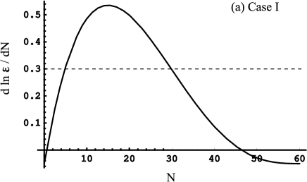
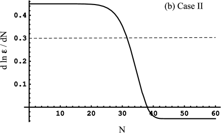
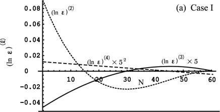
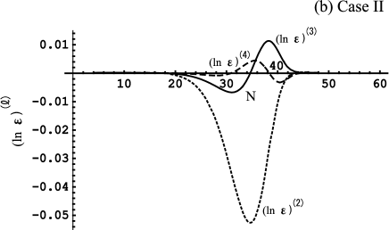
In Fig. 3 we plot the schematic pictures in case I (top) and case II (bottom), respectively. In figure 5 we show the derivatives of $d\ln\epsilon/dN$ with respect to $N$. The hierarchy (35) is in general respected except where the denominators pass through zero.

We impose the observational constraints on ${{\cal P}_{\zeta}}$, $n$ and $n^{\prime}$. To be on the safe side we also impose a rough finite-difference version of the constraint on $n^{\prime}$ in the following way. The WMAP data spans a range roughly $\ell\sim{\cal O}(1)$ – ${\cal O}(10^{3})$, corresponding to $\Delta N\sim 7$ $(\equiv\Delta N$, and $n$ derived from that data has an error of about $0.1$. Therefore, we require that $n$ should change by less than 0.02 in the range $N_{0}$ to $N_{0}-\Delta N$. We have checked that the condition (60) needed for the PBH production is satisfied with all of the observational constrains for $p=1$, $q=3$, $B\simeq 5.5$, $D\simeq 0.05$, $N_{0}=60$ and $\Delta N=5$ for Case I, and $q=10$, $A=5$, $B\simeq 0.5$, $D\simeq 0.05$, $N_{0}=50$ and $\Delta N=10$ for Case II. For the detailed numerical values of $n$ and $n^{\prime}$, see Table 1. It is clear that with a parameterisation like the one in Figure 3, we can make $n$ practically constant over the range $\Delta N\sim 10$ of scales probed by large-scale observations.

	$n(N_{0})$	$n(N_{0}-\Delta N$)	$n^{\prime}(N_{0})$	$n^{\prime}(N_{0}-\Delta N)$
Case I	0.9500	0.9529	0	0.0017
Case II	0.9500	0.9511	$1.4942\times 10^{-15}$	$5.9700\times 10^{-16}$

Table 1: $n$ and $n^{\prime}$ at $N=N_{0}$ and $N=N_{0}-\Delta N$ in Case I and Case II.

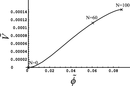
For the parameterisation I, the potential has a scaling $V_{0}\propto(\phi-\phi_{0})^{2}$. We plot it in Figure 4. Note that $V_{0}^{1/4}/M_{p}$ should be less than $\sim 10^{-3}$ for the slow-roll inflation $\epsilon\ll 1/N_{0}$ and $\phi<M_{p}$. This shape is similar to those in some classes of hilltop inflation models hilltop .

Figure 3: Schematic pictures of functional form of y(N) in Case I (top) and Case II (bottom), respectively. For reference we also plot the constant case, $n=0.3$ (see the text).

Figure 4: Form of the potential $V$ as a function of the field $\phi$. The horizontal axis is the normalized value of $\phi$, $\tilde{\phi}=\left[\frac{\phi-\phi_{0}}{M_{p}}\right]/\left[\frac{V_{0}^{1/4}}{M_{p}}/10^{-3}\right]^{2}$ with $\phi_{0}\equiv\phi(0)$ and $V_{0}\equiv V(\phi_{0})$. The vertical axis means $\tilde{V}=\left[\frac{V}{V_{0}}-1\right]/\left[\frac{V_{0}^{1/4}}{M_{p}}/10^{-3}\right]^{4}$.

Figure 5: Derivatives of $d(\ln\epsilon)/dN$ with respect to $N$ for Case I (top) and Case II (bottom), respectively. Here we plot the higher derivatives (ln $\epsilon)^{(\ell)}=d^{(\ell)}(\ln\epsilon)/dN^{(\ell)}$ for $\ell$ = 2, 3, and 4.

Figure 6: Two scenarios for generating black holes using a curvaton-type paradigm.

IX Black hole formation in a curvaton-type paradigm

The inflaton contribution $\zeta_{i}(k)$ is time-independent, and is the only one present at horizon exit. Subsequently though, the contribution $\zeta_{c}(t,k)$ of some other (curvaton-type) field could grow and become dominant. (See mycurv for a discussion of the possibilities with extensive references.) Eventually $\zeta(t)$ will level out to the observed value;

$$\zeta(k)=\zeta_{i}(k)+\zeta_{c}(k),$$ (65)

where the last term is the eventual time-independent value of the curvaton-type contribution. In an obvious notation, the observed spectrum is now

$${{\cal P}_{\zeta}}={\cal P}_{i}+{\cal P}_{c},$$ (66)

and the spectral index is

$$n-1=f_{i}(n_{i}-1)+f_{c}(n_{c}-1),$$ (67)

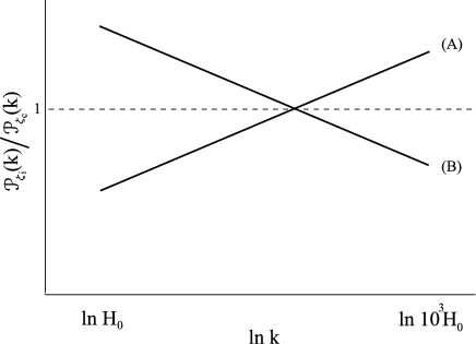
where $f_{i}={\cal P}_{i}/{{\cal P}_{\zeta}}$ and $f_{c}={\cal P}_{c}/{{\cal P}_{\zeta}}$. We will consider two different possibilities for the ratio ${\cal P}_{i}(k)/{\cal P}_{\rm c}(k)$, illustrated in Figure 6.

IX.1 Black holes from the inflaton perturbation

We first assume that $f_{c}\ll 1$ at the end of inflation so that black holes are generated by the inflaton perturbation, but that $f_{i}\ll 1$ while cosmological scales leave the horizon. To agree with observation, we will demand at $N=N_{0}$

$$n_{c}-1\simeq n-1\simeq 0.05,$$ (68)

and

$$f_{i}|n_{i}-1|<1\times 10^{-2}.$$ (69)

To form black holes, Eq. (60) becomes

$$14 = \ln[{{\cal P}_{\zeta}}(0)/{\cal P}_{c}(N_{0})]$$ (70)

$$= \ln[{{\cal P}_{\zeta}}(0)/{{\cal P}_{\zeta}}(N_{0})]+\ln[f_{i}(0)]$$ (71)

$$= (n_{i}-1)N+\ln(f_{i}(0)),$$ (72)

where we set $n_{i}^{\prime}=0$ to get the last line. These requirements are satisfied with, for example, $f_{i}(0)\simeq 10^{-1}$ and $n_{i}\simeq 1.4$, and the observational bound on the running imposes no further constraint.

The required spectral index $n_{i}$ corresponds to $\eta=0.2$ which is more or less compatible with the slow-roll requirement $|\eta|\ll 1$. In the context of supergravity such a value is more natural than the small value $\eta=-0.025$ required to fit observation. This looks promising for black hole formation, but we have to remember that in a curvaton type model the prediction for $n$ becomes mycurv

$$n-1 = 2\eta_{\sigma\sigma}-2\epsilon$$ (73)

$$\eta_{\sigma\sigma} \equiv -\frac{1}{3H_{*}^{2}}\frac{\partial^{2}V}{\partial\sigma^{2}}.$$ (74)

If $\epsilon$ is negligible as we are assuming, this requires $\eta_{\sigma\sigma}=-0.025$ which may difficult to achieve since $\sigma$ will tend to roll away from any maximum of its potential mycurv . In a curvaton type model it may therefore be more attractive al to take $\eta_{\sigma\sigma}$ negligible and $\epsilon=0.025$, but we have not explored that option.

IX.2 Black holes from the curvaton-type contribution

Now we suppose that the roles of the inflaton and the curvaton are reversed, so that the inflaton generates the observation curvature perturbation while the curvaton perturbation generates black holes. In this case black hole generation occurs only when the curvaton-type mechanism operates which will usually be long after inflation is over.

In this scenario, we have to modify Eqs. (69)–(72) by interchanging $i$ and $c$, and replacing the epoch $N=0$ by an earlier epoch $N_{\rm curv}$. This is the epoch at which the scale leaves the horizon, that is entering the horizon when the curvaton mechanism operates. To achieve black hole formation we will therefore generally need $n_{c}>1.4$, but that need not be a problem. Indeed, within the context of supergravity a value $n_{c}$ significantly bigger than 1 is expected mycurv , just as it is for $n_{i}$. This, our third scenario for generating black holes, therefore seems at least as good as the other two.

A particularly interesting possibility in this case, is that the curvature perturbation generating the black holes could easily be highly non–gaussian, to be precise the square of a gaussian quantity mycurv . This would not make much of a change hidalgo in the magnitude of ${{\cal P}_{\zeta}}$ needed to generate black holes (upon which our estimates are based) but it could alter the predicted shape of the black hole mass function.

X Conclusion

The possibility of primordial black hole formation at the end of inflation has a long history, which was long overdue for an update. The update is needed partly because observation now requires on cosmological scales a tilt far below $0.3$ (and with negative sign) and not too much running. It is also needed because the original paradigm, that the inflaton perturbation is entirely responsible for the curvature perturbation, is now only one possibility.

According to the standard paradigm, the curvature perturbation is generated during slow roll inflation from the vacuum fluctuation of the inflaton field. Within this paradigm, the running-mass model provides a well-motivated way of achieving black hole formation. To form black holes, the model probably requires strong running on cosmological scales, $n^{\prime}\sim 0.01$.

Such running is allowed by the data. If a value $n^{\prime}\sim 10^{-2}$ on cosmological scales is ruled out in the future, $n^{\prime}$ will still have to increase to $\gtrsim 10^{-2}$ in order to form black holes. We saw that this may be achieved within the standard paradigm by a suitable potential. Alternatively, it might be achieved by a switch from the standard paradigm to a curvaton-type paradigm, or by a switch from the curvaton-type paradigm to the standard paradigm.

For observers, we would like to re-iterate and earlier conclusion paris , that an upper bound $n^{\prime}<10^{-3}$, or detection, would have important implications and is a very worthwhile goal.

XI Acknowledgements

We thank Will Kinney and Andrew Liddle for comments on the draft of this paper. The research at Lancaster is supported by PPARC grant PP/D000394/1 and by EU grants MRTN-CT-2004-503369 and MRTN-CT-2006-035863.

References

- (1) D. H. Lyth, K. A. Malik and M. Sasaki, JCAP 0505, 004 (2005);
- (2) D. N. Spergel et al., Astrophys. J. Suppl. 170, 377 (2007).
- (3) D. H. Lyth, arXiv:0707.0361 [astro-ph].
- (4) B. J. Carr and S. W. Hawking, Mon. Not. Roy. Astron. Soc. 168, 399 (1974); B. J. Carr, Astrophys. J. 201, 1 (1975); K. Kohri and J. Yokoyama, Phys. Rev. D 61, 023501 (2000); B. J. Carr, In the Proceedings of 22nd Texas Symposium on Relativistic Astrophysics at Stanford University, Stanford, California, 13-17 Dec 2004, pp 0204, [arXiv:astro-ph/0504034]; I. Zaballa, A. M. Green, K. A. Malik and M. Sasaki, JCAP 0703, 010 (2007), [arXiv:astro-ph/0612379].
- (5) B. J. Carr, J. H. Gilbert and J. E. Lidsey, Phys. Rev. D 50 (1994) 4853 [arXiv:astro-ph/9405027]. H. I. Kim and C. H. Lee, Phys. Rev. D 54 (1996) 6001. A. M. Green and A. R. Liddle, Phys. Rev. D 56 (1997) 6166 [arXiv:astro-ph/9704251]. M. Lemoine, Phys. Lett. B 481, 333 (2000) [arXiv:hep-ph/0001238]. A. M. Green, Phys. Rev. D 60 (1999) 063516 [arXiv:astro-ph/9903484].
- (6) M. Sasaki and E. D. Stewart, Prog. Theor. Phys. 95, 71 (1996) [arXiv:astro-ph/9507001].
- (7) D. H. Lyth and A. Riotto, Phys. Rept. 314, 1 (1999).
- (8) D. H. Lyth, JCAP 0606 (2006) 015 [arXiv:astro-ph/0602285].
- (9) A. D. Linde , Phys. Lett. B 327, 208 (1994); astro-ph/9402031; A. Vilenkin, Phys. Rev. Lett. 72, 3137 (1994). hep-th/9402085.
- (10) A. D. Linde and V. Mukhanov, Phys. Rev. D 56 (1997) 535 [arXiv:astro-ph/9610219]; D. H. Lyth and D. Wands, Phys. Lett. B 524, 5 (2002) [arXiv:hep-ph/0110002]; T. Moroi and T. Takahashi, Phys. Lett. B 522 (2001) 215 [Erratum-ibid. B 539 (2002) 303] [arXiv:hep-ph/0110096]; D. H. Lyth, C. Ungarelli and D. Wands, Phys. Rev. D 67 (2003) 023503 [arXiv:astro-ph/0208055]; S. Mollerach, Phys. Rev. D 42, 313 (1990).
- (11) A. A. Starobinsky, JETP Lett. 42, 152 (1985) [Pisma Zh. Eksp. Teor. Fiz. 42, 124 (1985)]; D. H. Lyth and Y. Rodriguez, Phys. Rev. Lett. 95 (2005) 121302.
- (12) E. D. Stewart, Phys. Lett. B 391, 34 (1997) E. D. Stewart, Phys. Rev. D 56, 2019 (1997)
- (13) L. Covi, D. H. Lyth and L. Roszkowski, Phys. Rev. D 60, 023509 (1999) L. Covi and D. H. Lyth, Phys. Rev. D 59, 063515 (1999) L. Covi and D. H. Lyth, Mon. Not. Roy. Astron. Soc. 326, 885 (2001); D. H. Lyth and L. Covi, Phys. Rev. D 62, 103504 (2000).
- (14) L. Covi, D. H. Lyth and A. Melchiorri, Phys. Rev. D 67, 043507 (2003).
- (15) L. Covi, D. H. Lyth, A. Melchiorri and C. J. Odman, Phys. Rev. D 70, 123521 (2004).
- (16) W. H. Kinney, E. W. Kolb, A. Melchiorri and A. Riotto, Phys. Rev. D 74 (2006) 023502
- (17) R. Easther and H. Peiris, JCAP 0609 (2006) 010
- (18) F. Finelli, M. Rianna and N. Mandolesi, JCAP 0612 (2006) 006
- (19) J. Martin and C. Ringeval, JCAP 0608 (2006) 009
- (20) S. M. Leach, I. J. Grivell and A. R. Liddle, Phys. Rev. D 62, 043516 (2000)
- (21) M. Kawasaki, T. Takayama, M. Yamaguchi and J. Yokoyama, Phys. Rev. D 74, 043525 (2006); G. Ballesteros, J. A. Casas and J. R. Espinosa, JCAP 0603, 001 (2006).
- (22) A. Lewis and S. Bridle, Phys. Rev. D 66, 103511 (2002). Available at the website: cosmologist.info
- (23) L. Page et al. [WMAP Collaboration], Astrophys. J. Suppl. 170, 335 (2007).
- (24) G. Hinshaw et al. [WMAP Collaboration], Astrophys. J. Suppl. 170, 288 (2007).
- (25) N. Jarosik et al. [WMAP Collaboration], Astrophys. J. Suppl. 170, 263 (2007).
- (26) A. C. S. Readhead et al., Astrophys. J. 609, 498 (2004).
- (27) C. Dickinson et al., Mon. Not. Roy. Astron. Soc. 353, 732 (2004).
- (28) C. L. Kuo et al., American Astronomical Society Meeting, Vol. 201 (2002).
- (29) C. J. MacTavish et al., Astrophys. J. 647, 799 (2006).
- (30) S. Cole et al., Mon. Not. Roy. Astron. Soc. 362, 505 (2005).
- (31) T. Kawaguchi, M. Kawasaki, T. Takayama, M. Yamaguchi and J. Yokoyama, arXiv:0711.3886 [astro-ph].
- (32) A. R. Liddle and D. H. Lyth, Cosmological Inflation and Large Scale Structure, (CUP, Cambridge, 2000)
- (33) L. Alabidi and D. H. Lyth, JCAP 0605, 016 (2006)
- (34) D. H. Lyth, arXiv:hep-th/0702128.
- (35) A. H. Guth and S. Y. Pi, Phys. Rev. Lett. 49 (1982) 1110. A. A. Starobinsky, Phys. Lett. B 117 (1982) 175. J. M. Bardeen, P. J. Steinhardt and M. S. Turner, Phys. Rev. D 28 (1983) 679.
- (36) A. R. Liddle and D. H. Lyth, Phys. Lett. B 291 (1992) 391;
- (37) V. F. Mukhanov, JETP Lett. 41, 493 (1985); M. Sasaki, Prog. Theor. Phys. 76, 1036 (1986).
- (38) E. D. Stewart and D. H. Lyth, Phys. Lett. B 302, 171 (1993) [arXiv:gr-qc/9302019].
- (39) J. O. Gong and E. D. Stewart, Phys. Lett. B 510, 1 (2001).
- (40) E. D. Stewart, Phys. Rev. D 65, 103508 (2002) [arXiv:astro-ph/0110322].
- (41) J. Maldacena, JHEP 0305, 013 (2003) [arXiv:astro-ph/0210603]; D. Seery and J. E. Lidsey, JCAP 0509, 011 (2005) [arXiv:astro-ph/0506056]; D. Seery, J. E. Lidsey and M. S. Sloth, JCAP 0701, 027 (2007) [arXiv:astro-ph/0610210]; D. Seery, J. E. Lidsey and M. S. Sloth, JCAP 0701, 027 (2007) [arXiv:astro-ph/0610210].
- (42) W. H. Kinney, Phys. Rev. D 66, 083508 (2002).
- (43) A. R. Liddle, P. Parsons and J. D. Barrow, Phys. Rev. D 50, 7222 (1994) [arXiv:astro-ph/9408015].
- (44) S. Chongchitnan and G. Efstathiou, JCAP 0701, 011 (2007)
- (45) A. R. Liddle, Phys. Rev. D 68, 103504 (2003) [arXiv:astro-ph/0307286].
- (46) L. Boubekeur and D.H. Lyth, JCAP 0507, 010 (2005); K. Kohri, C. M. Lin and D. H. Lyth, JCAP (2007) in press, arXiv:0707.3826 [hep-ph].
- (47) J. C. Hidalgo, arXiv:0708.3875 [astro-ph].