Effective action, magnetic excitations and quantum fluctuations in lightly doped single layer cuprates

Abstract

We consider the extended 2D $t-t^{\prime}-t^{\prime\prime}-J$ model at zero temperature. Parameters of the model corresponds to doping by holes. Using the low doping effective action we demonstrate that the system can 1) preserve the long range collinear antiferromagnetic order, 2) lead to a spin spiral state (static or dynamic), 3) lead to the phase separation instability. We show that at parameters of the effective action corresponding to the single layer cuprate La_2-xSr_xCuO₄ the spin spiral ground state is realized. We derive properties of magnetic excitations and calculate quantum fluctuations. Quantum fluctuations destroy the static spin spiral at the critical doping $x_{c}\approx 0.11$. This is the point of the quantum phase transition to the spin-liquid state (dynamic spin spiral). The state is still double degenerate with respect to the direction of the dynamic spiral, so this is a “directional nematic”. The superconducting pairing exists throughout the phase diagram and is not sensitive to the quantum phase transition. We also compare the calculated neutron scattering spectra with experimental data.

I Introduction

The phase diagram of the prototypical cuprate superconductor La_2-xSr_xCuO₄ (LSCO) shows that the magnetic state changes tremendously with Sr doping. The three-dimensional antiferromagnetic (AF) Néel order identified keimer92 below $325\ \text{K}$ in the parent compound disappears at doping $x\approx 0.02$ and gives way to the so-called spin-glass phase which extends up to $x\approx 0.055$. In both, the Néel and the spin-glass phase, the system essentially behaves as an Anderson insulator and exhibits only hopping conductivity. Superconductivity then sets in for doping $x\gtrsim 0.055$, see Ref. kastner98 . One of the most intriguing properties of LSCO is the static incommensurate magnetic ordering observed at low temperature in elastic neutron scattering experiments. This ordering manifests itself as a scattering peak shifted with respect to the antiferromagnetic position. Very importantly, the incommensurate ordering is a generic feature of LSCO. According to experiments in the Néel phase, the incommensurability is almost doping independent and directed along the orthorhombic $b$ axis matsuda02 . In the spin-glass phase, the shift is also directed along the $b$ axis, but scales linearly with doping wakimoto99 ; matsuda00 ; fujita02 . Finally, in the underdoped superconducting region ($0.055\lesssim x\lesssim 0.12$), the shift still scales linearly with doping, but it is directed along the crystal axes of the tetragonal lattice yamada98 . Very recent studies reveal also the evolution of inelastic neutron spectra with doping yamada07 .

Near $x=0.12$ certain La-based materials develop a strongly enhanced static incommensurate magnetic order accompanied by small lattice deformation at the second order harmonics Tranquada95 ; Tranquada96 ; Fujita04 , see also Ref. tranquada05 for a review.

Incommensurate features have also been observed in inelastic neutron scattering from YBa₂Cu₃O_6+y (YBCO) bourges00 ; fong00 ; mook02 ; hayden04 ; hinkov04 ; stock06 ; hinkov07a . In underdoped YBCO there is a rather large uncertainty in the determining of the doping level. However, it seems that the incommensurability in YBCO is about 30-40% smaller than that in LSCO comparing the same doping level. In a very recent work hinkov07b the electronic liquid crystal state in underdoped YBCO has been reported. The state has no static spins, but nevertheless, it demonstrates a degeneracy with respect to the direction of the dynamic spin structure. In addition, there are indications that the electronic liquid crystal state observed in hinkov07b is very close to a quantum phase transition to a state with static spins.

The 2D $t-J$ model was suggested two decades ago to describe the essential low-energy physics of high-$T_{c}$ cuprates PWA ; Em ; ZR . In its extended version, this model includes additional hopping matrix elements $t^{\prime}$ and $t^{\prime\prime}$ to 2nd and 3rd-nearest Cu neighbors. The Hamiltonian of the $t-t^{\prime}-t^{\prime\prime}-J$ model on the square Cu lattice has the form:

$$H = -t\sum_{\langle ij\rangle\sigma}c_{i\sigma}^{{\dagger}}c_{j\sigma}-t^{\prime}\sum_{\langle ij^{\prime}\rangle\sigma}c_{i\sigma}^{{\dagger}}c_{j^{\prime}\sigma}-t^{\prime\prime}\sum_{\langle ij^{\prime\prime}\rangle\sigma}c_{i\sigma}^{{\dagger}}c_{j^{\prime\prime}\sigma}$$ (1)

$$+ J\sum_{\langle ij\rangle\sigma}\left(\mathbf{S}_{i}\mathbf{S}_{j}-{\frac{1}{4}}N_{i}N_{j}\right).$$

Here, $c_{i\sigma}^{{\dagger}}$ is the creation operator for an electron with spin $\sigma$ $(\sigma=\uparrow,\downarrow)$ at site $i$ of the square lattice, $\langle ij\rangle$ indicates 1st-, $\langle ij^{\prime}\rangle$ 2nd-, and $\langle ij^{\prime\prime}\rangle$ 3rd-nearest neighbor sites. The spin operator is $\mathbf{S}_{i}={\frac{1}{2}}c_{i\alpha}^{{\dagger}}\mathbf{\sigma}_{\alpha\beta}c_{i\beta}$, and $N_{i}=\sum_{\sigma}c_{i\sigma}^{{\dagger}}c_{i\sigma}$ with $\langle N_{i}\rangle=1-x$ being the number density operator. In addition to the Hamiltonian (1) there is the constraint of no double occupancy, which accounts for strong electron correlations. The values of the parameters of the Hamiltonian (1) for LSCO are known from neutron scattering keimer92 , Raman spectroscopy tokura90 and ab-initio calculations andersen95 . The values are: $J\approx 140\,\text{meV}$, $t\approx 450\,\text{meV}$, $t^{\prime}\approx-70\,\text{meV}$ , and $t^{\prime\prime}\approx 35\,\text{meV}$. Hereafter we set $J=1$, hence we measure energies in units of $J$.

The idea of spin spirals in the $t-J$ model at finite doping was first suggested in Ref. shraiman88 . The idea had initially attracted a lot of attention, see e. g. Refs. Dom ; IF ; CM . However, it has been soon realized that there was a fundamental unresolved theoretical problem of stability of the spiral CM . Together with lack of experimental confirmations this was a very discouraging development. The observation of static and quasistatic incommensurate peaks in neutron scattering caused a renewal of theoretical interest in the idea of spin spirals in cuprates hasselmann04 ; sushkov04 ; juricic04 ; sushkov05 ; lindgard05 ; juricic06 ; luscher06 ; luscher07 ; luscher07b . It has been realized that in LSCO the charge disorder related to a random distribution of Sr ions plays a crucial role and in the insulating state, $x\leq 0.055$, the disorder qualitatively influences the problem of stability of the spiral. The point is that in the insulating state the mobile holes are not really mobile, they are trapped in shallow hydrogen-like bound states near Sr ions. The trapping leads to the diagonal spin spiral sushkov05 ; luscher06 ; luscher07 ; luscher07b . Percolation of the bound states gives way to superconductivity and in the percolated state the spin spiral must be directed along crystal axes of the tetragonal lattice sushkov05 . So the percolation concentration is $x_{per}=0.055$. The rotation of the direction of the spin spiral is dictated by the Pauli exclusion principle. The disorder at $x>0.055$ is still pretty strong. However, unlike in the insulating phase, the disorder does not play a qualitative role and therefore in the first approximation one can disregard it. Thus, we arrive at the case of small uniform doping. This is the problem we address in the present work.

As we already mentioned, the case of an uniform spin spiral (no external disorder) in a doped quantum antiferromagnet has an inherent theoretical problem. If considered in the semiclassical approximation, the out-of-plane magnon is marginal and in the end this implies an instability of the spin spiral CM . An attempt to fix the problem by account of quantum fluctuations within the 1/S spin-wave theory was done in Ref. sushkov04 . We understand now that, while being qualitatively correct, the work sushkov04 did not account for all relevant quantum fluctuations. The effective action method is much more powerful then the 1/S expansion because the method accounts for all symmetries exactly and generates a regular expansion in powers of doping x, this is the true chiral perturbation theory. This is why in the present work we employ the effective action method.

The structure of the paper is the following. In section II we discuss the effective low-energy action of the modified t-J model. Section III addresses the issue of stability of the Néel state under doping. The spiral ground state in the mean-field approximation is considered in section IV. The in-plane magnons are discussed in section V and out-of-plane magnons in section VI. Section VII addresses the quantum fluctuations and the quantum phase transition to the directional nematic. Finally discussion and comparison with experiments is presented in the section VIII.

II Effective low-energy action of 2D $t-t^{\prime}-t^{\prime\prime}-J$ model at small doping

At zero doping (no holes), the $t$-$J$ model is equivalent to the Heisenberg model and describes the Mott insulator La₂CuO₄. The removal of a single electron from this Mott insulator, or in other words the injection of a hole, allows the charge carrier to propagate. Single-hole properties of the $t$-$J$ model are well understood, see Ref. dagotto94 for a review. A calculation of the hole dispersion at values of parameters $t$, $t^{\prime}$, and $t^{\prime\prime}$ corresponding to the single layer cuprate LSCO has been performed in Ref. sushkov04 using the Self Consistent Born Approximation (SCBA), see also Ref. luscher06 . According to this calculation the dispersion of the hole dressed by magnetic quantum fluctuations has minima at the nodal points $\mathbf{q}_{0}=(\pm\pi/2,\pm\pi/2)$, and it is practically isotropic in the vicinity of each point,

$$\epsilon\left(\mathbf{p}\right)\approx\frac{1}{2}\beta\mathbf{p}^{2}\ ,$$ (2)

where ${\bf p}={\bf q}-\mathbf{q}_{0}$. We set the lattice spacing to unity, 3.81 Å$\,\rightarrow$  1. The SCBA approximation gives $\beta\approx 2.2\approx 300\,\text{meV}$ . The effective mass corresponding to this value is approximately twice the electron mass and this agrees with recent measurement of Shubnikov - de Haas oscillations SdH . In the present work we use $\beta$ as a fitting parameter. We will see that to fit inelastic neutron data at $x=0.1$ we need

$$\beta\approx 2.7\ .$$ (3)

This agrees well with the value obtained within the SCBA. The quasi-particle residue $Z$ at the minimum of the dispersion is $Z\approx 0.38$ sushkov04 . In the full-pocket description, where two half-pockets are shifted by the AF vector ${\bf Q}_{AF}=\left(\pi,\pi\right)$, the two minima are located at $S_{a}=\left(\frac{\pi}{2},\frac{\pi}{2}\right)$ and $S_{b}=\left(\frac{\pi}{2},-\frac{\pi}{2}\right)$. The system is thus somewhat similar to a two-valley semiconductor.

The relevant energy scale for small uniform doping at zero temperature is of the order of $xJ\ll J$, relevant momenta are also small, $q\ll 1$. Hence, one can simplify the Hamiltonian of the $t$-$J$ model by integrating out all high-energy fluctuations. This procedure leads to the effective Lagrangian or effective action. The effective Lagrangian has been first discussed quite some time ago wiegman88 ; wen89 ; shraiman88 , see also a recent work W . That discussion resulted in the kinematic structure of the effective Lagrangian valid in the static limit shraiman88 . This limit is sufficient only for the mean-field approximation. The time-dependent terms that are necessary for excitations and quantum fluctuations have been derived only recently luscher07b . The effective Lagrangian can be written in terms of the bosonic ${\vec{n}}$-field that describes the staggered component of the copper spins and in terms of fermionic holons $\psi$. We use the term “holon” instead of “hole” because spin and charge are to some extent separated, see discussion below. The holon has a pseudospin that originates from two sublattices, so the fermionic field $\psi$ is a spinor acting on pseudospin. For the hole-doped case, the effective Lagrangian reads

$${\cal L} = \frac{\chi_{\perp}}{2}{\dot{\vec{n}}}^{2}-\frac{\rho_{s}}{2}\left({\bm{\nabla}}{\vec{n}}\right)^{2}$$

$$+ \sum_{\alpha}\left\{\frac{i}{2}\left[\psi^{{\dagger}}_{\alpha}{{\cal D}_{t}\psi}_{\alpha}-{({\cal D}_{t}\psi_{\alpha})}^{{\dagger}}\psi_{\alpha}\right]\right.$$

$$- \left.\psi^{{\dagger}}_{\alpha}\epsilon_{\alpha}({\bf\cal P})\psi_{\alpha}+\sqrt{2}g(\psi^{{\dagger}}_{\alpha}{\vec{\sigma}}\psi_{\alpha})\cdot\left[{\vec{n}}\times({\bm{e}}_{\alpha}\cdot{\bm{\nabla}}){\vec{n}}\right]\right\}\ .$$

The first two terms in the Lagrangian represent the usual nonlinear $\sigma$ model (NLSM), the field ${\vec{n}}$ is the subject of the constraint $n^{2}=1$. The magnetic susceptibility and the spin stiffness are $\chi_{\perp}\approx 0.53/8\approx 0.066$ and $\rho_{s}\approx 0.18$ SZ . The rest of the Lagrangian in Eq. (II) represents the fermionic holon field and its interaction with the ${\vec{n}}$-field. The coupling constant is IF , $g\approx Zt\approx 1$. The index $\alpha=a,b$ (flavor) indicates the location of the holon in momentum space (either in pocket $S_{a}$ or $S_{b}$). The kinematic structure of the coupling term was first derived in Ref. shraiman88 . The operator ${\vec{\sigma}}$ is a pseudospin that originates from the existence of two sublattices and ${\bf e}_{\alpha}=(1/\sqrt{2},\pm 1/\sqrt{2})$ is a unit vector orthogonal to the face of the MBZ where the holon is located. Kinetic energy of the holon, $\epsilon_{\alpha}({\bf p})$, is quadratic in the momentum ${\bf p}$ and generally speaking it can be anisotropic. However, in LSCO the anisotropy is small and we use the isotropic approximation (2).

A very important point is that the argument of $\epsilon$ in Eq. (II) is a “long” (covariant) momentum shraiman88 ,

$${\bf{\cal P}}=-i{\bm{\nabla}}+\frac{1}{2}{\vec{\sigma}}\cdot[{\vec{n}}\times{\bm{\nabla}}{\vec{n}}]\ .$$ (5)

An even more important point is that the time derivatives that stay in the kinetic energy of the fermionic field are also “long” (covariant) luscher07b ,

$${\cal D}_{t}=\partial_{t}+\frac{i}{2}{\vec{\sigma}}\cdot[{\vec{n}}\times{\dot{\vec{n}}}]\ .$$ (6)

The covariant time derivatives result in the “Berry phase term”  luscher07b , $-\frac{1}{2}\psi_{\alpha}^{{\dagger}}{\vec{\sigma}}\psi_{\alpha}\cdot[{\vec{n}}\times{\dot{\vec{n}}}]$, that is crucially important for excitation spectrum and hence for stability of the system with respect to quantum fluctuations.

Generally speaking, there are also quartic in fermion operators terms in the effective Lagrangian. However, these terms are not important at low doping and therefore we disregard them in (II).

The effective Lagrangian (II) is valid regardless if the ${\vec{n}}$-field is static or dynamic. In other words it does not matter if the ground state expectation value of the staggered field is nonzero, $\langle{\vec{n}}\rangle\neq 0$, or zero, $\langle{\vec{n}}\rangle=0$. The only condition for validity of (II) is that all dynamic fluctuations of the ${\vec{n}}$-field are slow, $1/\tau\ll J$ , where $\tau$ is the typical time-scale of the fluctuations. We will demonstrate below that the dimensionless parameter

$$\lambda=\frac{2g^{2}}{\pi\beta\rho_{s}}$$ (7)

plays an important role in the theory. If $\lambda\leq 1$, the ground state corresponding to the Lagrangian (II) is the collinear Néel state and it stays collinear at any small doping. If $1\leq\lambda\leq 2$, the Néel state is unstable at arbitrary small doping and the ground state is static or dynamic spin spiral. Whether the spin spiral is static or dynamic depends on doping. If $\lambda\geq 2$, the system is unstable with respect to phase separation and hence the effective long-wave-length Lagrangian (II) is meaningless. Thus,

$$\lambda \leq 1\ ,\ \ \ Neel\ \ state$$

$$1\leq \lambda \leq 2\ ,\ \ \ Spiral\ state\ ,\ static\ or\ dynamic$$ (8)

$$\lambda \geq 2,\ \ \ Phase\ \ separation\ .$$

For LSCO the value is $\lambda\approx 1.3-1.5$.

We would like to stress once more that spin and charge to some extent are separated in the effective low-energy Lagrangian (II), this is why we use the term “holon” instead of “hole”. The holon carries pseudospin, it carries charge, but it does not carry spin in the usual sense. However, it is not the full spin-charge separation like in 1D models. To illustrate this point, it is instructive to look at the holon interaction with uniform external magnetic field luscher06 ; luscher07b .

$$\delta{\cal L}_{B}=\frac{1}{2}({\vec{B}}\cdot{\vec{n}})\psi^{{\dagger}}_{\alpha}({\vec{\sigma}}\cdot{\vec{n}})\psi_{\alpha}\ .$$ (9)

Since we only want to stress the spin dynamics this interaction does not include terms that originate from the long derivative with respect to magnetic vector potential $-i{\bm{\nabla}}\to-i{\bm{\nabla}}-\frac{e}{c}{\bf A}$, describing the interaction of the magnetic field with the electric charge. Clearly the interaction (9) is quite unusual and this is what we call “the partial spin-charge separation”. The holon does not interact directly with the staggered magnetic field (neutron scattering).

III Criterion of stability of the Néel phase under doping

One can consider the coupling constant $g$ in the Lagrangian (II) as a formal parameter. It is clear that the Néel order must be stable at a sufficiently small $g$,

$${\vec{n}}\approx{\vec{n}}_{0}=(0,0,1)\ .$$ (10)

In this case the two hole pockets are populated by holons with pseudospin “up” and “down”, and hence the Fermi momentum (radius of the pocket) is

$$p_{F}=\sqrt{\pi x}\ ,$$ (11)

where $x$ is doping.

Figure 1: Magnon-holon vertex, magnon is shown by the dashed line

The Lagrangian (II) can be split in the diagonal and offdiagonal part with respect to transverse spin waves $n_{\perp}=n_{\pm}=(n_{x}\pm in_{y})/\sqrt{2}$.

$${\cal L} ={\cal L}_{0}+{\cal L}_{1}\ ,$$ (12)

$${\cal L}_{0} =\frac{\chi_{\perp}}{2}{\dot{n}_{\perp}}^{2}-\frac{\rho_{s}}{2}\left(1+\frac{\beta x}{4\rho_{s}}\right)\left({\bm{\nabla}}{n_{\perp}}\right)^{2}+\sum_{\alpha}\left(\frac{i}{2}\left[\psi^{{\dagger}}_{\alpha}{\dot{\psi}}_{\alpha}-{\dot{\psi}}_{\alpha}^{{\dagger}}\psi_{\alpha}\right]-\psi^{{\dagger}}_{\alpha}\epsilon({\bf p})\psi_{\alpha}\right)\ ,$$

$${\cal L}_{1} =\sum_{\alpha}\psi_{\alpha}^{{\dagger}}\left(-\frac{1}{2}{\vec{n}}_{0}[{\dot{\vec{n}}_{\perp}}\times{\vec{\sigma}}]-\frac{\beta}{4}\left\{{{\bm{p}}},{\vec{n}}_{0}[{\bm{\partial}}{\vec{n}}_{\perp}\times{\vec{\sigma}}]\right\}+\sqrt{2}g{\vec{n}}_{0}[({\bm{e}}_{\alpha}\cdot{\bm{\nabla}}{\vec{n}}_{\perp})\times{\vec{\sigma}}]\right)\psi_{\alpha}\ .$$

Here $\left\{...,...\right\}$ stands for the anticommutator. Using the second quantization representation for the ${\vec{n}}$-field,

$$n_{\pm}=\sum_{\bf q}\frac{1}{\sqrt{2\chi_{\perp}\omega_{\bf q}}}\left(e^{i\omega_{\bf q}t-i{\bf q}\cdot{\bf r}}m_{\pm,\bf q}^{{\dagger}}+e^{-i\omega_{\bf q}t+i{\bf q}\cdot{\bf r}}m_{\pm,\bf q}\right)\ ,$$

with the magnon creation and annihilation operators $m_{\pm,\bf q}^{{\dagger}}$ and $m_{\pm,\bf q}$, we find the “bare” magnon dispersion

$$\omega_{\bf q}^{2}=c^{2}q^{2}\left(1+\frac{\beta x}{4\rho_{s}}\right)\ ,\ \ \ c^{2}=\frac{\rho_{s}}{\chi_{\perp}}\ ,$$ (13)

and the pseudospin flip magnon-holon vertex shown in Fig. 1,

$$M=i\sqrt{\frac{2}{\chi_{\perp}}}\left\{\sqrt{2}g({\bf e}_{\alpha}\cdot{\bf q})+\frac{\omega}{2}+\frac{1}{2}[\epsilon({\bf p})-\epsilon({\bf p}+{\bf q})]\right\}\ .$$ (14)

Looking at (13), one can conclude superficially that magnons are hardened by doping. However, they are not hardened, they are softened. To see this we need to calculate the magnon polarization operator that is due to ${\cal L}_{1}$. The operator reads

$${\cal P}_{N}(\omega,{\bf q}) = \frac{2}{\chi_{\perp}}\sum_{{\bf p},\alpha}f_{\bf p}(1-f_{{\bf p}+{\bf q}})\frac{\left\{\sqrt{2}g({\bf e}_{\alpha}\cdot{\bf q})+\frac{\omega}{2}+\frac{1}{2}[\epsilon({\bf p})-\epsilon({\bf p}+{\bf q})]\right\}^{2}}{\epsilon({\bf p})+\omega-\epsilon({\bf p}+{\bf q})+i0}$$ (15)

$$+ \frac{2}{\chi_{\perp}}\sum_{{\bf p},\alpha}f_{\bf p}(1-f_{{\bf p}-{\bf q}})\frac{\left\{\sqrt{2}g({\bf e}_{\alpha}\cdot{\bf q})+\frac{\omega}{2}+\frac{1}{2}[\epsilon({\bf p}-{\bf q})-\epsilon({\bf p})]\right\}^{2}}{\epsilon({\bf p})-\omega-\epsilon({\bf p}-{\bf q})+i0}\ ,$$

where $f_{\bf p}$ is the usual Fermi-Dirac step function. Eq. (15) can be transformed to

$${\cal P}_{N}(\omega,{\bf q}) = -\frac{\beta c^{2}x}{4\rho_{s}}q^{2}+2{\cal P}_{0}(\omega,{\bf q})\ ,$$

$${\cal P}_{0}(\omega,{\bf q}) = \frac{2c^{2}g^{2}}{\rho_{s}}q^{2}\sum_{{\bf p}}f_{\bf p}(1-f_{{\bf p}+{\bf q}})\left(\frac{1}{\epsilon({\bf p})+\omega-\epsilon({\bf p}+{\bf q})+i0}+\frac{1}{\epsilon({\bf p})-\omega-\epsilon({\bf p}+{\bf q})+i0}\right)\ .$$ (16)

Then the magnon Green’s function reads

$$G=\frac{\chi_{\perp}^{-1}}{\omega^{2}-\omega_{\bf q}^{2}-{\cal P}(\omega,{\bf q})+i0}=\frac{\chi_{\perp}^{-1}}{\omega^{2}-c^{2}q^{2}-2{\cal P}_{0}(\omega,{\bf q})+i0}\ .$$ (17)

The condition of stability of the ground state is the absence of poles of the Green’s function at imaginary $\omega$-axis. Hence this condition is $c^{2}q^{2}\geq-2{\cal P}_{0}(0,{\bf q})=\lambda c^{2}q^{2},\ \ at\ \ q\ll p_{F}$. Doping $x$ does not appear in this criterion. Thus, as it is stated in (II), the Néel state is stable at any small doping if $\lambda\leq 1$. This criterion has been discussed many times, see e.g.sushkov04 . We have rederived it here just to demonstrate how the effective action technique works in the known situation.

IV The spiral ground state in the mean-field approximation

At $\lambda\geq 1$ the minimum energy is realized with the coplanar spiral

$${\vec{n}}_{0}=(\cos{\bf Q}\cdot{\bf r},\ \sin{\bf Q}\cdot{\bf r},\ 0)\ ,$$ (18)

where ${\bf Q}\propto(1,0);(0,1)$ is directed along the CuO bond. To be specific we assume that ${\bf Q}\propto(1,0)$. Due to the holon interaction with the spiral the holon band is split in two with $\sigma_{z}=\pm 1$,

$$\epsilon \to -\frac{\Delta}{2}\sigma_{z}+\frac{1}{2}\beta\left({\bf p}+\frac{1}{2}{\bf Q}\sigma_{z}\right)^{2}\ ,$$

$$\Delta = 2gQ\ .$$ (19)

In the ground state only the band with $\sigma_{z}=+1$ is populated. Therefore, the Fermi momentum, that is the radius of the Fermi circle in each pocket, is

$$p_{F}=\sqrt{2\pi x}\ .$$ (20)

The point ${\bf p=0}$ corresponds to ${\bf k}=(\pi/2,\pm\pi/2)$ in the Brillouin zone. According to (IV) the center of the filled holon pocket ($\sigma_{z}=1)$ is shifted from this point by $-\frac{1}{2}{\bf Q}$, and the center of the empty pocket ($\sigma_{z}=-1)$ is shifted by $\frac{1}{2}{\bf Q}$. Calculation of energy and its minimization with respect to $Q$ gives the following value

$$Q=\frac{g}{\rho_{s}}x\ .$$ (21)

The ground state energy of the spiral state is below that of the Néel state only if $\lambda\geq 1$.

V The in-plane magnons in the spiral state

To analyze the stability of the spiral state one needs to go beyond the mean-field approximation and study excitations and quantum fluctuations in the system. In this section we consider in-plane magnetic excitations. An in-plane excitation is described by a small deviation $\varphi=\varphi(t,{\bf r})$ from the uniform spiral ground state (18),

$${\vec{n}}=(\cos({\bf Q\cdot r}+\varphi),\sin({\bf Q\cdot r}+\varphi),0)\ .$$ (22)

In the ground state all the holons are in the pseudospin state $\sigma_{z}=1$. The in-plane magnons do not change pseudospin, therefore in this section we set everywhere $\sigma_{z}=1$. Substituting expression (22) in the Lagrangian (II) we once more find the diagonal and offdiagonal parts of the Lagrangian

$${\cal L} = {\cal L}_{0}+{\cal L}_{1}\ ,$$ (23)

$${\cal L}_{0} = \frac{\chi_{\perp}}{2}{\dot{\varphi}}^{2}-\frac{\rho_{s}}{2}\left(1+\frac{\beta x}{4\rho_{s}}\right)\left({\bm{\nabla}}{\varphi}\right)^{2}$$

$$+ \sum_{\alpha}\left(\frac{i}{2}\left[\psi^{{\dagger}}_{\alpha}{\dot{\psi}}_{\alpha}-{\dot{\psi}}_{\alpha}^{{\dagger}}\psi_{\alpha}\right]-\psi^{{\dagger}}_{\alpha}\left[-\frac{\Delta}{2}+\epsilon({\bf l}^{2})\right]\psi_{\alpha}\right)\ ,$$

$${\cal L}_{1} = \sum_{\alpha}\psi_{\alpha}^{{\dagger}}\psi_{\alpha}\left(\sqrt{2}g({\bm{e}}_{\alpha}\cdot{\bm{\nabla}})\varphi-\frac{1}{2}{\dot{\varphi}}-\frac{\beta}{4}\left\{{\bm{l}},{\bm{\partial}}\varphi\right\}\right)\ .$$

Here ${\bf l}={\bf p}+{\bf Q}/2$ is shifted momentum and $\left\{...,...\right\}$ stands for anticommutator. Thus, the “bare” magnon dispersion is given by the same Eq. (13) as for the Néel state, but the magnon-holon vertex is smaller than (14) by the factor $\sqrt{2}$,

$$M =i\sqrt{\frac{1}{\chi_{\perp}}}\left\{\sqrt{2}g({\bf e}_{\alpha}\cdot{\bf q})+\frac{\omega}{2}+\frac{1}{2}[\epsilon({\bf l})-\epsilon({\bf l}+{\bf q})]\right\}\ .$$ (24)

A calculation similar to that performed in section III for the Néel state gives the following Green’s function for the field $\varphi$ that describes the in-plane magnon

$$G_{in}=\frac{\chi_{\perp}^{-1}}{\omega^{2}-c^{2}q^{2}-{\cal P}_{0}+i0}\ ,$$ (25)

where ${\cal P}_{0}$ is given by Eq. (III) with the Fermi momentum (20). At zero frequency and at small $q$, $q\ll p_{F}$, the polarization operator is equal to ${\cal P}_{0}(0,{\bf q})=-\frac{\lambda}{2}c^{2}q^{2}$. Therefore, the ground state is getting unstable (poles of the Green’s function at imaginary $\omega$-axis) at $\lambda\geq 2$. This is the instability with respect to phase separation CM ; sushkov04 and it is fatal for the effective long-wave-length Lagrangian (II). Thus, the spiral state is stable at $1\leq\lambda\leq 2$, see Eq. (II). We also present here an explicit expression for the polarization operator

$${\text{Re}}\ {\cal P}_{0}(\omega,q) = -\frac{c^{2}g^{2}}{\pi\beta^{2}\rho_{s}}\left\{\beta q^{2}-R_{1}\sqrt{1-R_{0}^{2}/R_{1}^{2}}\ \ \theta(1-R_{0}^{2}/R_{1}^{2})-R_{2}\sqrt{1-R_{0}^{2}/R_{2}^{2}}\ \ \theta(1-R_{0}^{2}/R_{2}^{2})\right\}\ ,$$

$${\text{Im}}\ {\cal P}_{0}(\omega,q) = -\frac{c^{2}g^{2}}{\pi\beta^{2}\rho_{s}}\left\{\theta(R_{0}^{2}-R_{1}^{2})\ \sqrt{R_{0}^{2}-R_{1}^{2}}-\sqrt{R_{0}^{2}-R_{2}^{2}}\ \theta(R_{0}^{2}-R_{2}^{2})\right\}\ ,$$

$$R_{0} = \beta qp_{F}\ ,\ \ \ R_{1}=\frac{1}{2}\beta q^{2}-\omega\ ,\ \ \ R_{2}=\frac{1}{2}\beta q^{2}+\omega\ .$$ (26)

The Fermi momentum $p_{F}$ is given by (20), and $\theta(x)$ is the usual step function.

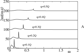
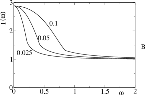
Figure 2: A: Plots of $2\omega I_{in}(\omega,q)$ versus energy for different values of momentum $q$ (offsets). $I_{in}(\omega,q)$ is the in-plane magnon spectral density (27). The plots are presented for doping $x=0.1$, and $\beta=2.7$, $g=1$. Values of $q$ are given in units of the incommensurate vector $Q$, see (21).
B: $q$-integrated in-plane spectral density (28) for dopings $x=0.025$, $0.05$, and $0.1$. The parameters of the effective Lagrangian are $\beta=2.7$, $g=1$.

It is convenient to define the magnon spectral density as

$$I_{in}(\omega,{\bf q})=-4\rho_{s}\text{Im}G_{in}(\omega,q)\ .$$ (27)

Plots of $2\omega I_{in}(\omega,{\bf q})$ versus $\omega$ are presented in Fig. 2A for different values of momentum $q$ (offsets). The doping is $x=0.1$, and $\beta=2.7$, $g=1$. The narrow peak is the $\delta$-function broadened “by hands” to fit in the picture size. The corresponding quasiparticle residue is rather small, say for $q=0.1Q$ in Fig. 2A the residue is $Z=0.39$ and it very quickly dies out at larger values of $q$. The magnon “dissolves” in the particle-hole continuum.

The $q$-integrated in-plane magnon spectral density

$$I_{in}(\omega)=\int I_{in}(\omega,{\bf q})\frac{d^{2}q}{(2\pi)^{2}}$$ (28)

is plotted in Fig. 2B for doping $x=0.025$, $x=0.05$, and $x=0.1$. For zero energy the value of the $q$-integrated spectral density is independent of doping and equals to $I_{in}(0)=1/(1-\lambda/2)$.

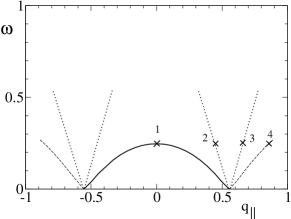
Figure 3: The magnon dispersion along Q. The parameters are $x=0.1$, $\beta=2.7$, $g=1$. The out-of-plane excitation for $|q|\leq Q$ is shown by the solid line and the out-of-plane excitation for $|q|\geq Q$ is shown by the dashed line. The in-plane excitation is shown by the dotted line. The quasiparticle residue decays very quickly outside of the dome shown by the solid line. The quasiparticle residue at point 1 at the top of the dome is $Z=0.8$ while the quasiparticle residue at point 4 that is outside of the dome at the same height is just $Z=0.13$. The quasiparticle residue of the in-plane magnon at the same frequency as the dome height (points 2 and 3) is $Z=0.15$.

To calculate the in-plane spectral density that can be observed in neutron scattering one needs to shift momenta. The Hamiltonian describing the interaction of the neutron spin ${\vec{S}}^{N}$ with the ${\vec{n}}$-field reads

$$H^{N}\propto{\vec{S}}^{N}\cdot{\vec{n}}=S^{N}_{z}n_{z}+\frac{1}{2}\left(S^{N}_{+}n_{-}+S^{N}_{-}n_{+}\right)\ .$$ (29)

After the substitution of the in-plane excitation (22), the above Hamiltonian reads

$$H^{N} \propto\frac{1}{2}S^{N}_{+}e^{-i({\bf Q}\cdot{\bf r}+\varphi)}+\frac{1}{2}S^{N}_{-}e^{i({\bf Q}\cdot{\bf r}+\varphi)}$$

$$\to\frac{1}{2}e^{i{\bf k}\cdot{\bf r}}\left\{S^{N}_{+}e^{-i{\bf Q}\cdot{\bf r}}(1-i\varphi)+S^{N}_{-}e^{i{\bf Q}\cdot{\bf r}}(1+i\varphi)\right\}\ ,$$

where ${\bf k}$ is the momentum transfer and ${\bf Q}$ the momentum shift due to the spiral ground state. The scattering probability for unpolarized neutrons is given by

$${\cal I}_{in}(\omega,{\bf k})=\frac{1}{2}\left[I_{in}(\omega,{\bf k}-{\bf Q})+I_{in}(\omega,{\bf k}+{\bf Q})\right]\ .$$ (30)

In Fig. 3 we show by dotted lines the brunches of linear dispersion that correspond to the quasiparticle peak in the spectral function $I_{in}(\omega,{\bf q})$ plotted in Fig. 2A. The dispersion is very steep, steeper than the bare magnon velocity $c$, and the corresponding intensities are very low.

VI The out-of-plane magnons in the spiral state

Dynamics of out-of-plane magnons are the most complicated ones. Stability of the spiral state was questioned because of the “marginal” character of the out-of-plane excitations if considered in semiclassical 1/S-approximation shraiman88 ; CM . The effective action technique allows us to resolve the problem because the technique accounts exactly all the symmetries.

Figure 4: Magon-holon vertexes with pseudospin flip, magnon is shown by the dashed line

For the out-of-plane excitation let us write the ${\vec{n}}$-field as

$${\vec{n}}=(\sqrt{1-n_{z}^{2}}\cos{\bf Q}\cdot{\bf r},\sqrt{1-n_{z}^{2}}\sin{\bf Q}\cdot{\bf r},n_{z})\ ,$$

and substitute this expression into the effective Lagrangian (II). Neglecting cubic and higher order terms in $n_{z}$, we get the diagonal and the offdiagonal parts of the Lagrangian

$${\cal L} ={\cal L}_{0}+{\cal L}_{1}\ ,$$ (31)

$${\cal L}_{0} =\frac{\chi_{\perp}}{2}{\dot{n}_{z}}^{2}-\frac{\rho_{s}}{2}\left(1+\frac{\beta x}{4\rho_{s}}\right)\left[Q^{2}n_{z}^{2}+\left({\bm{\nabla}}{n}_{z}\right)^{2}\right]+\sum_{\alpha}\left(\frac{i}{2}\left[\psi^{{\dagger}}_{\alpha}{\dot{\psi}}_{\alpha}-{\dot{\psi}}_{\alpha}^{{\dagger}}\psi_{\alpha}\right]-\psi^{{\dagger}}_{\alpha}\left[-\frac{\Delta}{2}\sigma_{z}+\frac{\beta}{2}\left({\bf p}+\frac{1}{2}{\bf Q}\sigma_{z}\right)^{2}\right]\psi_{\alpha}\right)\ ,$$

$${\cal L}_{1} =-\sum_{\alpha}\psi^{{\dagger}}_{\alpha}\frac{\sigma_{+}}{2}\left(e^{-i{\bf Q}\cdot{\bf r}}\left[g[Qn_{z}-i\sqrt{2}({\bm{e}}_{\alpha}\cdot{\bm{\nabla}})n_{z}]+\frac{i}{2}{\dot{n}}_{z}\right]-\frac{\beta}{4}\left\{{\bm{p}},e^{-i{\bf Q}\cdot{\bf r}}[{\bm{Q}}n_{z}-i{\bm{\partial}}n_{z}]\right\}\right)\psi_{\alpha}+h.c.\ .$$

Here $\sigma_{+}=\sigma_{x}+i\sigma_{y}$ and the bracket $\left\{...,...\right\}$ stands for anticommutator. According to (31), the “bare” magnon dispersion in this case is

$$\omega_{b,\bf q}^{2}=c^{2}(Q^{2}+q^{2})\left(1+\frac{\beta x}{4\rho_{s}}\right)\ .$$ (32)

The interaction ${\cal L}_{1}$ generates the following two pseudospin-flip vertexes shown in Fig. 4  ,

$$M_{a} = i\sqrt{\frac{1}{\chi_{\perp}}}\left\{g[Q-\sqrt{2}({\bf e}_{\alpha}\cdot{\bf q})]-\frac{\omega}{2}-\frac{\beta}{4}\left[(2{\bf p}+{\bf Q}+{\bf q})\cdot({\bf Q}-{\bf q})\right]\right\}\ ,$$

$$M_{b} = i\sqrt{\frac{1}{\chi_{\perp}}}\left\{g[Q+\sqrt{2}({\bf e}_{\alpha}\cdot{\bf q})]+\frac{\omega}{2}-\frac{\beta}{4}\left[(2{\bf p}+{\bf Q}-{\bf q})\cdot({\bf Q}+{\bf q})\right]\right\}\ .$$ (33)

Hence, the magnon polarization operator determined by the vertexes reads

$${\cal P}(\omega,{\bf q})=$$ (34)

$$=\frac{2}{\chi_{\perp}}\sum_{{\bf l}}f_{\bf l}\left(\frac{\left[g(Q-q_{||})-\frac{\omega}{2}-\frac{\beta}{4}(2{\bf l}+{\bf q})\cdot({\bf Q}-{\bf q})\right]^{2}+g^{2}q_{\perp}^{2}}{\epsilon({\bf l})-\epsilon({\bf l}+{\bf q})+\omega-\Delta+i0}+\frac{\left[g(Q+q_{||})+\frac{\omega}{2}-\frac{\beta}{4}(2{\bf l}-{\bf q})\cdot({\bf Q}+{\bf q})\right]^{2}+g^{2}q_{\perp}^{2}}{\epsilon({\bf l})-\epsilon({\bf l}-{\bf q})-\omega-\Delta+i0}\right)\ .$$

Here $q_{||}$ and $q_{\perp}$ are components of momentum parallel and perpendicular to ${\bf Q}$, respectively; $f_{\bf l}$ is the Fermi-Dirac step function and ${\bf l}={\bf p}+{\bf Q}/2$ is the shifted momentum. Eq. (34) can be transformed to

$${\cal P}(\omega,{\bf q})=-\frac{\beta c^{2}x}{4\rho_{s}}q^{2}-c^{2}Q^{2}+$$

$$+ \frac{2c^{2}}{\rho_{s}}\sum_{{\bf l}}f_{\bf l}\left(\left[gq_{||}+\frac{\beta}{2}{\bf Q}\cdot({\bf l}+{\bf q}/2)\right]^{2}+g^{2}q_{\perp}^{2}\right)\left(\frac{1}{\epsilon({\bf l})-\omega-\epsilon({\bf l}+{\bf q})-\Delta+i0}+\frac{1}{\epsilon({\bf l})+\omega-\epsilon({\bf l}+{\bf q})-\Delta+i0}\right)\ .$$

This form is explicitly symmetric with respect to $\omega\to-\omega$ and ${\bf q}\to-{\bf q}$. Integration in (VI) leads to the following magnon Green’s function

$$G_{out} = \frac{\chi_{\perp}^{-1}}{\omega^{2}-\omega_{b,\bf q}^{2}-{\cal P}(\omega,{\bf q})+i0}$$

$$= \chi_{\perp}^{-1}\left[\omega^{2}-2c^{2}Q^{2}\frac{q_{\perp}^{2}}{q^{2}}\left(1-\frac{Q^{2}}{q^{2}}\right)-c^{2}q^{2}\left(1-\frac{Q^{2}}{q^{2}}\right)^{2}+\frac{c^{2}}{\pi\beta^{2}\rho_{s}}(F_{+}+F_{-})+i0\right]^{-1}\,,$$

where

$$\mbox{Re}\,F_{+}=\frac{A}{4q^{2}}R_{\Delta}\left[1-\sqrt{1-\frac{R_{0}^{2}}{R_{\Delta}^{2}}}\,\theta\left(1-\frac{R_{0}^{2}}{R_{\Delta}^{2}}\right)\right]+\frac{Q^{2}q_{\perp}^{2}}{6q^{6}}R_{\Delta}^{3}\left[1-\sqrt{1-\frac{R_{0}^{2}}{R_{\Delta}^{2}}}\left(1+\frac{R_{0}^{2}}{2R_{\Delta}^{2}}\right)\,\theta\left(1-\frac{R_{0}^{2}}{R_{\Delta}^{2}}\right)\right]\,,$$

$$\mbox{Im}\,F_{+}=\sqrt{R_{0}^{2}-R_{\Delta}^{2}}\,\theta\left(1-\frac{R_{\Delta}^{2}}{R_{0}^{2}}\right)\left\{\frac{A}{4q^{2}}+\frac{Q^{2}q_{\perp}^{2}}{6q^{6}}\left(\frac{R_{0}^{2}}{2}+R_{\Delta}^{2}\right)\right\}\,,$$

$$A=4g^{2}q^{2}+q_{\parallel}^{2}Q^{2}\left[\frac{\beta^{2}}{4}+\frac{2g\beta}{Q}-\frac{R_{\Delta}}{q^{2}}\left(\frac{4g}{Q}+\beta\right)\right]+\frac{R_{\Delta}^{2}Q^{2}}{q^{4}}(q_{\parallel}^{2}-q_{\perp}^{2})\,,$$

$$R_{\Delta}=\Delta-\omega+\frac{1}{2}\beta q^{2}\,.$$ (37)

Here $\theta(x)$ is the step function and $R_{0}$ is defined in (V). The function $F_{-}$ is obtained from $F_{+}$ by the replacement $\omega\to-\omega$ in $R_{\Delta}$.

We define the out-of-plane magnon spectral density as

$$I_{out}(\omega,{\bf q})=-4\rho_{s}\text{Im}\ G_{out}(\omega,q)\ .$$ (38)

Plots of $2\omega I_{out}(\omega,{\bf q})$ versus $\omega$ are presented in Fig. 5A for different values of momentum $q_{||}$ (offsets) and $q_{\perp}=0$. The doping is $x=0.1$.

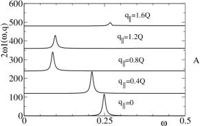
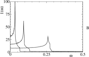
Figure 5: A: Plots of $2\omega I_{out}(\omega,q)$ versus energy for different values of momentum $q$ (offsets). $I_{out}(\omega,q)$ is the out-of-plane magnon spectral density (38). The plots are presented for doping $x=0.1$ and $\beta=2.7$, $g=1$. Values of $q$ are given in units of the incommensurate vector $Q$, see (21).
B: $q$-integrated in-plane spectral density (40) for dopings $x=0.025$, $0.05$, and $0.1$. The parameters are $\beta=2.7$, $g=1$.

The narrow peak is the $\delta$-function broadened “by hands”, the effective width is the same as that for in-plane magnons in Fig. 2. The corresponding quasiparticle dispersion $\Omega_{\bf q}$ is plotted in Fig. 3 for direction along ${\bf Q}$, (i.e. $q=q_{||}$, $q_{\perp}=0$) and for $x=0.1$. The part for $|q|\leq Q$ is shown by the solid line and the part for $|q|\geq Q$ is shown by the dashed line. We do it to stress that the quasiparticle residue decays very quickly outside of the dome. Plot of the residue is shown in Fig. 6A.

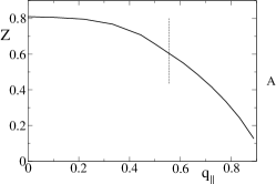
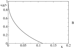
Figure 6: A: The quasiparticle residue versus momentum for the out-of-plane magnon for the direction along the spiral, $q=q_{||}$, $q_{\perp}=0$. The vertical line shows the momentum where the dispersion vanishes. The doping is $x=0.1$.
B: The static component of $n$-field versus doping. The parameters are $g=1$, $\beta=2.7$.

To illustrate intensities we compare points 1-4 in Fig. 3 which correspond to different brunches of dispersion with the same frequency. The quasiparticle residue at point 1 at the top of the dome is $Z=0.8$ while the quasiparticle residue at point 4 that is outside of the dome at the same height is $Z=0.13$. The quasiparticle residue of the in-plane magnon at the same frequency as the dome height (points 2 and 3 in Fig. 3) is $Z=0.15$.

An analysis of Eq. (VI) gives the following approximate formulas for the dispersion of the out-of-plane magnon and for the corresponding quasiparticle residue

$$\Omega_{\bf q}^{2} \approx \frac{\beta xQ^{2}c^{2}}{4\rho_{s}}\left(1-\frac{1}{\lambda}\right)\frac{\left(1-\frac{q^{2}}{Q^{2}}\right)^{2}+2\frac{q_{\perp}^{2}}{Q^{2}}}{1+\frac{c^{2}q^{2}}{4g^{2}Q^{2}}}\ ,$$

$$Z \approx \frac{1}{1+\frac{c^{2}q^{2}}{4g^{2}Q^{2}}}\ .$$ (39)

These formulas have very limited region of validity since, as we already pointed out, at larger $q$ the magnon dissolves in the particle-hole continuum. At $x=0.1$ the equation (VI) for $\Omega_{\bf q}$ agrees reasonably well with the result of numerical calculation shown in Fig. 3. At the same time the formula (VI) for the quasiparticle residue only poorly agrees with numerics shown in Fig. 6A. Certainly at very small doping Eq. (VI) is accurate.

The $q$-integrated out-of-plane magnon spectral density

$$I_{out}(\omega)=\int I_{out}(\omega,{\bf q})\frac{d^{2}q}{(2\pi)^{2}}$$ (40)

is plotted in Fig. 5B for doping $x=0.025$, $x=0.05$, and $x=0.1$. It is peaked at energy $E_{cross}$ corresponding to the top of the dome in Fig. 3. Interestingly, the spectral density decays almost abruptly to its high frequency asymptotic value $I(\omega)\to 1$ as soon as the magnon is dissolved in the particle-hole continuum. The decay of the in-plane $q$-integrated spectral density shown in Fig. 2 is not that steep.

VII Quantum fluctuations and quantum phase transition to the dynamic spiral phase (directional nematic)

Due to in-plane and out-of plane quantum fluctuations the static component of the staggered field ${\vec{n}}$ is reduced,

$$\langle n\rangle\approx 1-\frac{1}{2}\langle\varphi^{2}\rangle-\frac{1}{2}\langle n_{z}^{2}\rangle\ .$$ (41)

Expectation values $\langle\varphi^{2}\rangle$ and $\langle n_{z}^{2}\rangle$ can be expressed in terms of Green’s function or in terms of q-integrated spectral densities

$$\langle\varphi^{2}\rangle = -\sum_{\bf q}\int\frac{d\omega}{2\pi i}G_{in}(\omega,{\bf q})=\frac{1}{4\rho_{s}}\int\frac{d\omega}{2\pi}I_{in}(\omega),$$ (42)

$$\langle n_{z}^{2}\rangle = -\sum_{\bf q}\int\frac{d\omega}{2\pi i}G_{out}(\omega,{\bf q})=\frac{1}{4\rho_{s}}\int\frac{d\omega}{2\pi}I_{out}(\omega)\ .$$

These expressions must be renormalized by subtraction of the ultraviolet-divergent contribution that corresponds to the undoped $\sigma$-model. The physical meaning of relations (41) and (42) is very simple: the reduction of static response is transferred to the dynamic response. The most important contribution to quantum fluctuations comes from out-of-plane excitations with momenta $q\sim Q\propto x$. To find this contribution we use the Green’s function $G_{out}\approx\frac{Z_{\bf q}}{\omega^{2}-\Omega_{\bf q}^{2}}$, where $Z$ and $\Omega$ are given by Eq. (VI). This gives

$$<n_{z}^{2}>\to\frac{gc}{\pi^{2}\sqrt{\beta}\rho_{s}^{3/2}\sqrt{1-1/\lambda}}{\cal B}\sqrt{x}\ ,$$ (43)

$${\cal B}=\frac{1}{2}\int_{0}^{\infty}\int_{0}^{\pi/2}\frac{dtd\varphi}{\sqrt{\left(1+\frac{c^{2}}{4g^{2}}t\right)\left[(1-t)^{2}+2t\cos^{2}\phi\right]}}\,.$$

Thus, the leading term in the quantum fluctuation scales as $\propto\sqrt{x}$. The subleading contribution to the quantum fluctuation scales is $x$. To find it we have performed numerical integration in Eq. (42) using q-integrated spectral densities $I_{out}$ and $I_{in}$ calculated in sections V and VI, see Fig. 2B and Fig. 5B. This gives

$$\langle n\rangle\approx 1-\frac{gc}{2\pi^{2}\sqrt{\beta}\rho_{s}^{3/2}\sqrt{1-1/\lambda}}{\cal B}\sqrt{x}+2.6x\ .$$ (44)

Certainly the coefficient in the subleading x-term depends on parameters (a rather weak dependence). The value 2.6 in (44) corresponds to $g=1$ and $\beta=2.7$. The plot of $\langle n\rangle$ versus doping $x$ at these values of parameters is presented in Fig. 6B.

According to Fig. 6B the static component of ${\vec{n}}$ vanishes at $x=x_{c}\approx 0.11$. This is a quantum critical point for transition to the dynamic spiral. In this phase there isn’t a spontaneous direction of the ${\vec{n}}$-field, $\langle{\vec{n}}\rangle=0$, but the spiral direction (1,0) or (0,1) is still spontaneously selected. In our opinion, this is the “nematic phase” observed in Ref. hinkov07b . Clearly the value $x_{c}\approx 0.11$ is an approximate value. In doing the spin-wave theory we assume that $\langle\varphi^{2}\rangle,\langle n_{z}^{2}\rangle\ll 1$, but then, to find the critical point we extend this consideration to $\langle n_{z}^{2}\rangle\sim 1$. This extension brings some uncertainty in the value of $x_{c}$. We also would like to note that the value of $x_{c}$ is rather sensitive to parameters. The main sensitivity comes from $\sqrt{1-1/\lambda}$ in the denominator in Eq. (44). The value of $\lambda$ given by Eq. (7) is closely related to the value of the incommensurate vector $Q$ given by Eq. (21). Our estimate of $x_{c}$ is valid for LSCO.

At $x\geq x_{c}$ the spin-wave pseudogap is opened. To describe the gapped phase we use the Takahashi approach takahashi , see also Ref. chandra . Idea of this approach is to impose constraint $\langle n\rangle=0$ using the Lagrange multiplier method. So we introduce an additional term in the effective Lagrangian

$$\delta{\cal L}=\chi_{\perp}\Delta_{s}^{2}\left(1-\frac{1}{2}\varphi^{2}-\frac{1}{2}n_{z}^{2}\right)\ ,$$ (45)

where $\Delta_{s}$ is technically the Lagrange multiplier, and physically this is the spin-wave pseudogap. The value of $\Delta_{s}$ must be determined from the condition

$$\langle n\rangle=1-\frac{1}{2}\langle\varphi^{2}\rangle-\frac{1}{2}\langle n_{z}^{2}\rangle=0\ .$$ (46)

The in-plane quantum fluctuation $\langle\varphi^{2}\rangle$ is only very weakly (quadratically) dependent on the pseudogap $\Delta_{s}$. The out-of-plane fluctuation $\langle n_{z}^{2}\rangle$ contains a term that depends on $\Delta_{s}$ linearly. The term comes from the $\sqrt{x}$-contribution in Eqs. (43),(44).

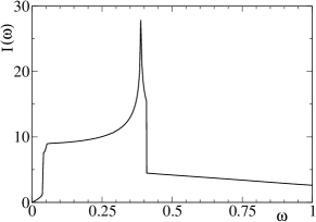
Figure 7: The $q$-integrated magnon spectral density $I=I_{in}+I_{out}$ in the gapped “nematic” phase for $x=0.13$ and $x_{c}=0.11$.

To account for the pseudogap one needs to replace the expression in square brackets under the square root in ${\cal B}$, see Eq. (43), by

$$\left[(1-t)^{2}+2t\cos^{2}\phi\right]+\frac{4g}{c^{2}\beta(1-1/\lambda)Q^{3}}\Delta_{s}^{2}\ .$$ (47)

A simple calculation with parameters $g=1$ and $\beta=2.7$ shows that the condition (46) results in the following pseud0gap

$$\Delta_{s}\approx 2.5(x-x_{c})\ .$$ (48)

This formula is valid only very close to the critical point. In this problem one cannot expect a high accuracy from the Takahashi-like approach. Therefore, the slope 2.5 in Eq. (48) is rather approximate. Finally, in Fig. 7 we present the plot of the q-integrated magnon spectral density $I_{in}(\omega)+I_{out}(\omega)$ for $x=0.13$ and $x_{c}=0.11$. The figure clearly demonstrates that $\Delta_{s}$ is a pseudogap since there is some spectral weight at $\omega\leq\Delta_{s}$.

VIII Discussion and comparison with experiment

There are several points that can be directly compared with experiment. The incommensurability vector $Q$ is given by equation (21). It depends on the coupling constant $g$. Fit of experimental incommensurability yamada98 gives $g\approx 1$ and this agrees remarkably well with prediction of the $t-t^{\prime}-t^{\prime\prime}-J$ model.

An important dynamical parameter is $E_{cross}$ which is the height of the dome in Fig. 3. This parameter has been systematically studied very recently in inelastic neutron scattering yamada07 . The experimental values are presented in Table I.

$x$	0.025	0.04	0.05	0.07	0.1
$E_{cross}(\mbox{meV})$	7 ${}^{+4}_{-2}$	15 ${}^{+7}_{-3}$	20 ${}^{+6}_{-5}$	23 ${}^{+9}_{-7}$	40 ${}^{+5}_{-5}$
phase	insulator			superconductor
spiral direction	diagonal			parallel
theory	Refs. luscher07 ; luscher07b			present work

Table 1: LSCO: Experimental values yamada07 of $E_{cross}$ versus doping $x$.

As soon as the coupling constant $g$ is found from the experimental incommensurability $Q$ we can fit $E_{cross}$. As we already pointed out above, the present theory is applicable to LSCO at $x\geq x_{per}\approx 0.055$. According to Eq. (VI)

$$E_{cross}\approx\sqrt{\frac{\beta xQ^{2}c^{2}}{4\rho_{s}}\left(1-\frac{1}{\lambda}\right)}\ .$$ (49)

Comparing this formula with data at $x=0.07$ and $x=0.1$ in Table I we find that $\beta=2.65(1\pm 0.1)$. This value agrees reasonably well with the value $\beta\approx 2.2$ that follows from the $t-t^{\prime}-t^{\prime\prime}-J$ model. Note that in principle the inverse mass $\beta$ can be somewhat dependent on doping. However, the data with error bars are quite consistent with x-independent $\beta$.

Let us discuss also the data at $0.02\leq x\leq x_{per}=0.055$ that is relevant to the insulating phase with diagonal disordered spin spiral. The corresponding theory has been developed in Refs. luscher07 ; luscher07b . The incommensurability in this case is $Q=\sqrt{2}gx/\rho_{s}$. To fit the experimental incommensurability we need $g\approx 0.7$. This is somewhat smaller than the value in the conducting phase. We believe that the reduction of $g$ is due to interaction with phonons. The point is that $g=Zt$, where $Z$ is the quasihole residue. Interaction with phonons in the insulating phase can easily reduce the residue by 20-30%. Stability of the disordered spiral in the insulating phase is due to localization of holes. The $E_{cross}$ in this case is luscher07b

$$E_{cross}\approx c\sqrt{\frac{3}{4}}\frac{Q^{2}}{\kappa}\ ,$$ (50)

where $\kappa$ is the inverse localization length. It is worth noting that Eq. (50) has been derived in Ref. luscher07b assuming that the binding energy of a hole trapped by Sr ion is larger than the magnon energy. The binding energy is about 10-15meV. Therefore, strictly speaking, Eq. (50) is applicable only at $x=0.025$ since at larger $x$ the energy $E_{cross}$ is getting too big. Nevertheless, we can try to apply (50) to the data at $x\leq 0.055$. Fitting the data from Table I we find values of $\kappa$, $x=0.025$: $\kappa=0.55\pm 0.2$, $x=0.04$: $\kappa=0.65\pm 0.2$, and $x=0.05$: $\kappa=0.75\pm 0.2$. So, there is a hint for a weak doping dependence of the inverse localization length $\kappa$. Most likely the dependence is just an imitation of the binding energy correction to formula (50). On the other hand, a weak dependence of the localization length on doping is quite possible. The above values agree reasonably well with the value $\kappa\approx 0.4$ that follows from the analysis of the variable range hopping conductivity at a very small doping ($x=0.002$), see Ref. chen95 .

Near $x=0.12$ certain La-based materials in LTT phase develop a strongly enhanced static incommensurate magnetic order accompanied by a small lattice deformation at the second order harmonics Tranquada95 ; Tranquada96 ; Fujita04 , see also Ref. tranquada05 for a review. The measured static magnetic moment $\sim 0.1\mu_{b}$ is substantially larger than the value that follows from the present theory (the unity in the vertical scale in Fig. 6B corresponds to the magnetic moment $0.6\mu_{B}$). There are also experimental indications that the spin structure in this case is close to collinear christensen . We strongly believe that physics of these materials is somehow related to mechanisms considered in the present paper. On the other hand, it is clear that in this case there are some additional effects that are not accounted for by the present theory.

The present theory qualitatively explains the directional nematic state discovered in underdoped YBCO at doping $x\approx 0.08$ hinkov07b . For a quantitative comparison one needs to analyse the two layer situation. This analysis has to include an explanation of a smaller incommensurability compared to that observed in the single layer LSCO.

In the present work we did not account for the superconducting pairing. The point is that at low doping the pairing practically does not influence magnetic excitations. A different question is how the spiral and the corresponding magnetic excitations influence the superconducting pairing. The spin-wave exchange mechanism for pairing of holons was suggested in Refs. flambaum ; belinicher . The mechanism is always working as soon as a short range antiferromagnetic order exists in the system. So the superconductivity peacefully coexists with spin spirals sushkov04 . Moreover, we understand now that the pairing in the spiral state is strongly enhanced by closeness to the Néel state instability driven by the parameter $\lambda$. The enhancement will be considered elsewhere.

In conclusion, using the low-energy effective field theory we have considered the 2D $t$-$J$ model in the limit of small doping. Quantitatively this consideration is relevant to underdoped single layer cuprates. We have derived the incommensurate spin structure (static and/or dynamic), calculated spectra of magnetic excitations (Figs. 2, 3, 5), and considered the quantum phase transition to the directional nematic spin-liquid phase. The spin wave pseudogap is opened in the spin-liquid phase, the q-integrated spectral density in this case is shown in Fig.7.

- (1) B. Keimer, A. Aharony, A. Auerbach, R. J. Birgeneau, A. Cassanho, Y. Endoh, R. W. Erwin, M. A. Kastner, and G. Shirane, Phys. Rev. B45, 7430 (1992).
- (2) M. A. Kastner, R. J. Birgeneau, G. Shirane, and. Y. Endoh, Rev. Mod. Phys. 70, 897 (1998).
- (3) M. Matsuda, M. Fujita, K. Yamada, R. J. Birgeneau, Y. Endoh, and G. Shirane, Phys. Rev. B65, 134515 (2002).
- (4) S. Wakimoto, G. Shirane, Y. Endoh, K. Hirota, S. Ueki, K. Yamada, R. J. Birgeneau, M. A. Kastner, Y. S. Lee, P. M. Gehring, and S. H. Lee, Phys. Rev. B60, R769 (1999).
- (5) M. Matsuda, M. Fujita, K. Yamada, R. J. Birgeneau, M. A. Kastner, H. Hiraka, Y. Endoh, S. Wakimoto, and G. Shirane, Phys. Rev. B62, 9148 (2000).
- (6) M. Fujita, K. Yamada, H. Hiraka, P. M. Gehring, S. H. Lee, S. Wakimoto, and G. Shirane, Phys. Rev. B65, 064505 (2002).
- (7) K. Yamada, C. H. Lee, K. Kurahashi, J. Wada, S. Wakimoto, S. Ueki, H. Kimura, Y. Endoh, S. Hosoya, G. Shirane, R. J. Birgeneau, M. Greven, M. A. Kastner, and Y. J. Kim, Phys. Rev. B57, 6165 (1998).
- (8) K. Yamada, private communication.
- (9) J. M. Tranquada et al, Nature 375, 561 (1995).
- (10) J. M. Tranquada et al, Phys. Rev. B 54, 7489 (1996).
- (11) M. Fujita et al, Phys. Rev. B 66, 184503 (2002); 70, 104517 (2004).
- (12) J. M. Tranquada, cond-mat/0512115.
- (13) P. Bourges, Y. Sidis, H. F. Fong, L. P. Regnault, J. Bossy, A. Ivanov, and B. Keimer, Science 288, 1234 (2000).
- (14) H. F. Fong, P. Bourges, Y. Sidis, L. P. Regnault, J. Bossy, A. Ivanov, D. L. Milius, I. A. Aksay, and B. Keimer, Phys. Rev. B61, 14773 (2000).
- (15) H. A. Mook, Pengcheng Dai, F. Dogan, Phys. Rev. Lett. 88, 097004 (2002).
- (16) S. M. Hayden, H. A. Mook, Pengcheng Dai, T. G. Perring, and F. Doǧan, Nature 429, 53 (2004)
- (17) V. Hinkov, S. Pailhès, P. Bourges, Y. Sidis, A. Ivanov, A. Kulakov, C. T. Lin, D. P. Chen, C. Bernhard, and B. Keimer, Nature 430, 650 (2004)
- (18) C. Stock, W. J. L. Buyers, Z. Yamani, C. L. Broholm, J.-H. Chung, Z. Tun, R. Liang, D. Bonn, W. N. Hardy, and R. J. Birgeneau, Phys. Rev. B73, 100504 (2006).
- (19) V. Hinkov, P. Bourges, S. Pailhes, Y. Sidis, A. Ivanov, C. D. Frost, T. G. Perring, C. T. Lin, D. P. Chen, B. Keimer, Nature Physics 3, 780 (2007).
- (20) V. Hinkov, D. Haug, B. Fauque, P. Bourges, Y. Sidis, A. Ivanov, C. Bernhard, C. T. Lin, B. Keimer, ??? (2007).
- (21) P. W. Anderson, Science 235, 1196 (1987).
- (22) V. J. Emery, Phys. Rev. Lett. 58, 2794 (1987).
- (23) F. C. Zhang and T. M. Rice, Phys. Rev. B 37, R3759 (1988).
- (24) Y. Tokura, S. Koshihara, T. Arima, H. Takagi, S. Ishibashi, T. Ido, and S. Uchida, Phys. Rev. B41, R11657 (1990).
- (25) O. K. Andersen, A. I. Liechtenstein, O. Jepsen, and F. Paulsen, J. Phys. Chem. Solids 56, 1573 (1995); E. Pavarini, I. Dasgupta, T. Saha-Dasgupta, O. Jepsen, and O. K. Andersen ,Phys. Rev. Lett. 87 047003 (2001).
- (26) B. I. Shraiman and E. D. Siggia, Phys. Rev. Lett. 61, 467 (1988); Phys. Rev. Lett. 62, 1564 (1989); Phys. Rev. B42, 2485 (1990).
- (27) T. Dombre, J. Phys. (France) 51, 847 (1990).
- (28) J. Igarashi and P. Fulde, Phys. Rev. B 45, 10419 (1992).
- (29) A. V. Chubukov and K. A. Musaelian, Rev. B 51, 12605 (1995).
- (30) N. Hasselmann, A. H. Castro Neto, and C. Morais Smith, Phys. Rev. B69, 014424 (2004).
- (31) O. P. Sushkov and V. N. Kotov, Phys. Rev. B70, 024503 (2004).
- (32) V. Juricic, L. Benfatto, A. O. Caldeira, and C. Morais Smith, Phys. Rev. Lett. 92, 137202 (2004).
- (33) O. P. Sushkov and V. N. Kotov, Phys. Rev. Lett. 94, 097005 (2005).
- (34) P.-A. Lindgård, Phys. Rev. Lett. 95, 217001 (2005).
- (35) V. Juricic, M. B. Silva-Neto, and C. Morais Smith, Phys. Rev. Lett. 96, 077004 (2006).
- (36) A. Lüscher, G. Misguich, A. I. Milstein, and O. P. Sushkov, Phys. Rev. B73, 085122 (2006).
- (37) A. Lüscher, A. I. Milstein, and O. P. Sushkov, Phys. Rev. Lett. 98, 037001 (2007).
- (38) A. Lüscher, A. I. Milstein, and O. P. Sushkov, Phys. Rev. B75, 235120 (2007).
- (39) N. Doiron-Leyraud, C. Proust, D. LeBoeuf, J. Levallois, J.-B. Bonnemaison, R. Liang, D. A. Bonn, W. N. Hardy, and L. Taillefer, Nature 447, 565 (2007).
- (40) E. Dagotto, Rev. Mod. Phys. 66, 763 (1994).
- (41) P. Wiegman, Phys. Rev. Lett. , 60, 821 (1988).
- (42) X. G. Wen, Phys. Rev. B39, 7223 (1989).
- (43) F. Kampfer, M. Moser, and U.-J. Wiese, Nucl. Phys. B 729, 317 (2005); C. Brugger, F. Kampfer, M. Moser, M. Pepe, and U.-J. Wiese, Phys. Rev. B 74, 224432 (2006).
- (44) R. R. P. Singh, Phys. Rev. B 39, 9760 (1989); Zheng Weihong, J. Oitmaa, and C. J. Hamer, Phys. Rev B 43, 8321 (1991).
- (45) M. Takahashi, Phys. Rev. Lett. 58, 168 (1987); Phys. Rev. B 40, 2494 (1989).
- (46) P. Chandra, P. Coleman, and A. I. Larkin, J. Phys.: Condens. Matter 2, 7933 (1990).
- (47) C. Y. Chen, E. C. Branlund, ChinSung Bae, K. Yang, M. A. Kastner, A. Cassanho, and R. J. Birgeneau, Phys. Rev. B 51, 3671 (1995).
- (48) N. B. Christensen, H. M. Ronnow, J. Mesot, R. A. Ewings, N. Momono, M. Oda, M. Ido, M. Enderle, D. F. McMorrow, A. T. Boothroyd, Phys. Rev. Lett. 98, 197003 (2007).
- (49) V. V. Flambaum, M. Yu. Kuchiev, and O. P. Sushkov, Physica C 227, 267-278 (1994).
- (50) V. Belinicher, A. Chernyshev, A. Dotsenko, and O. P. Sushkov, Phys. Rev. B, 51, 6076-6084. (1995).