Negative-weight percolation

Abstract

We describe a percolation problem on lattices (graphs, networks), with edge weights drawn from disorder distributions that allow for weights (or distances) of either sign, i.e. including negative weights. We are interested whether there are spanning paths or loops of total negative weight. This kind of percolation problem is fundamentally different from conventional percolation problems, e.g. it does not exhibit transitivity, hence no simple definition of clusters, and several spanning paths/loops might coexist in the percolation regime at the same time. Furthermore, to study this percolation problem numerically, one has to perform a non-trivial transformation of the original graph and apply sophisticated matching algorithms.

Using this approach, we study the corresponding percolation transitions on large square, hexagonal and cubic lattices for two types of disorder distributions and determine the critical exponents. The results show that negative-weight percolation is in a different universality class compared to conventional bond/site percolation. On the other hand, negative-weight percolation seems to be related to the ferromagnet/spin-glass transition of random-bond Ising systems, at least in two dimensions.

1 Introduction

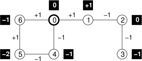
Percolation [13] is one of the most-fundamental problems in statistical mechanics. Many phase transitions in physical systems can be explained in terms of a percolation transition. The pivotal property of percolation is connectivity. One can describe this in terms of weighted graphs (often also called networks) with nonzero or zero weights, corresponding to occupied/connected or unoccupied/disconnected edges. Here, we extend the problem to negative weights, in particular we study bond percolation. As an example, one can imagine an agent traveling on a graph, who has, when traversing an edge, either to pay some resource (positive weight) or he is able (once) to harvest some resource (negative weight). Paths including negative edge weights also appear in the context of domain walls in random-bond Ising systems [10]. One percolation problem is whether there exists a path (or loop) spanning the full system with negative total weight, such that each edge is traversed at most once. Hence, the percolating objects are paths and it is sufficient to look for minimum-weighted (or “shortest”) paths (MWPs). Percolation properties of string-like objects have been studied occasionally [7, 12, 5, 14, 4, 11], but to our knowledge never allowing for negative weights. One realizes immediately that the negative weights lead to properties which are fundamentally different from conventional percolation. E.g., negative-weight percolation (NWP) lacks transitivity: If there is a valid (negative-weight) path $S\to A\to B$ from $S$ to $B$ via $A$, it is possible that the path $S\to A$ is not valid, as for the paths $0-1-2-3$/$0-1$ in figure 1. Hence, there is no simple definition of percolation clusters in this case. Note that, since strings are thus considered, several percolating strings or loops might coexist in the same sample. This we observe indeed, see below.

Here, we study NWP numerically. First we introduce the model. Then we outline the algorithm to obtain MWPs, since no standard shortest-path algorithm can be used. The results for different types of two- ($2d$) and three-dimensional ($3d$) systems, in particular the critical exponents describing the percolation transitions, show that NWP is fundamentally different compared to conventional percolation and from previous models with string-like percolation. Thus, the study of percolation models exhibiting negative weights might lead to many new insights concerning the behavior of disordered systems.

Figure 1: An example graph, exhibiting 7 nodes 0,$\ldots$,6 with positive and negative edge weights (numbers at lines). Numbers in black boxes denote the total weight of the minimum-weighted path from node 0 to the corresponding node.

2 Model and Algorithm

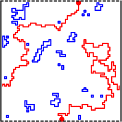
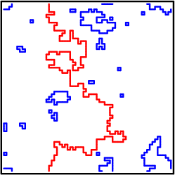
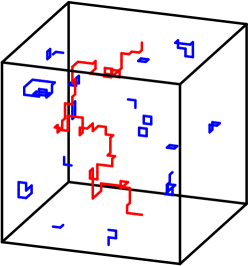
We consider $2d$ and $3d$ lattice graphs $G=(V,E)$ with side length $L$, where adjacent sites $i,j\in V$ are joined by undirected edges $e=(ij)\in E$. Weights $\omega(e)$ are associated with the edges, representing quenched random variables. We consider either bimodal ($\pm$J) or “Gaussian-like” (Gl) distribution of the edge weights, where $\rho$ denotes the fraction of negative or Gaussian-distributed edge weights, respectively, among edges with unit weight (fraction $1-\rho$). The bimodal weights are taken to be $\pm 1$ and the Gaussian weights have zero mean and unit width. These weight distributions explicitly allow for loops ${\mathcal{L}}$ with negative weight, given by $\omega_{\mathcal{L}}\!\equiv\!\sum_{e\in{\mathcal{L}}}\omega(e)$. For any non-zero value of $\rho$, a sufficiently large systems will exhibit at least small loops with negative total weight. We investigate (i) MWPs in the presence of negative weighted loops on square lattices with periodic boundary conditions (BCs) in one and free BCs in the other direction. The path ends are allowed to terminate on the free boundaries. Further, we study (ii) minimum-weighted configurations of negative-weighted loops on square, $2d$ hexagonal and cubic lattices with fully periodic BCs, see figure 2. In either case we find critical values of $\rho$ above which (i) negative-weight paths appear that span the lattice across the direction with periodic BCs or (ii) percolating loops emerge, that span the lattice along some direction.

Figure 2: Left: MWP (red) in the presence of negative-weight loops (blue) for $L\!=\!64$, middle (right): $2d$ ($3d$) loop configuration for $L\!=\!64~{}(24)$. Spanning loops are colored red. Each sample is taken slightly above the respective critical point $\rho_{c}$ for $\pm$J disorder. Dashed lines denote free BCs, solid lines indicate periodic BCs.

Since we are looking for MWPs on undirected graphs in the presence of negative weights, traditional “shortest path” algorithms cannot be applied. The reason is that for applying these traditional algorithms a special condition must hold: For the distance $d(i)$ of any shortest path from a source $0$ to $i\neq 0$, $d(i)=\min_{j\in N(i)}(d(j)+\omega(j,i))$ holds, where $N(i)$ denotes the set of neighbors of $i$. This equation is not fulfilled in our case, as can be seen from figure 1 for node $4$. It has minimum distance $-1$ to node $0$, but it is connected to node 5 via an edge of weight $\omega(5,4)\!=\!-1$ and $d(5)\!=\!-2$. Hence, a different approach has to be applied. We determine MWPs and loop configurations through an appropriate transformation of the original graph, detailed in [2], and obtaining a minimum-weighted perfect matching (MWPM) [6, 8], by using exact combinatorial optimization algorithms.

Here we give a concise description of the mapping, pictured as 3-step procedure illustrated in figure 3:

(1) each edge, joining 2 sites on $G$, is replaced by a path of 3 edges. Therefore, 2 “additional” sites have to be introduced for each edge of $G$. The original sites are then “duplicated” along with their incident edges. For each of these pairs of of duplicated sites, one additional edge is added that connect the two sites of a pair. The resulting auxiliary graph $G_{{\rm A}}$ is depicted in figure 3(b), where additional sites appear as squares and duplicated sites as circles. Figure 3(b) also illustrates the weight assignment on $G_{{\rm A}}$. A more extensive description can be found in [10].

(2) a MWPM on the auxiliary graph is determined [1]. A MWPM is a minimum-weighted subset $M$ of the edges contained in $G_{\rm A}$, such that each site of $G_{\rm A}$ is met by one edge in $M$. This is illustrated in figure 3(c), where the bold edges represent $M$ for the given weight assignment. The dashed edges are unmatched. Due to construction, the auxiliary graph consists of an even number of sites and since there are no isolated sites, it is guaranteed that a perfect matching exists.

(3) finally it is possible to find a relation between the matched edges $M$ on $G_{\rm A}$ and a configuration of negative-weighted loops $\mathcal{C}$ on $G$ by tracing the steps of the transformation (1) back. Note that each edge contained in $M$ that connects an additional site (square) to a duplicated site (circle) corresponds to an edge on $G$ that is part of a loop, see figure 3(d). More precise, there are always two such edges in $M$ that correspond to one edge on $G$. All the edges in $M$ that connect like sites (i.e. duplicated-duplicated, or additional-additional) carry zero weight and do not contribute to a loop on $G$. Afterwards a depht-first search can be used to explore $\mathcal{C}$ and to determine the properties of the individual loops. For the weight assignment in figure 3(a), there is only one loop with weight $\omega_{\mathcal{L}}\!=\!-2$ and length $\ell=4$.

Note that the result of the calculation is a collection $\mathcal{C}$ of loops (and one path for (i), see below), such that the total loop weight is minimized. Hence, one obtains a global collective optimum of the system. Clearly, all loops that contribute to $\mathcal{C}$ possess a negative weight. Note that $\mathcal{C}$ can be empty and that sub paths are neither allowed to intersect nor to terminate at some site within the lattice.

So as to induce a MWP, as in problem (i), special care is needed. We have to allow the paths explicitly to terminate at a certain node. Therefore, two extra sites are introduced to the graph. One extra site is connected to each of the free boundaries by adding edges with weight zero to the transformed graph that join the site with the sites of the respecting boundary. Any subsequent MWPM will contain a path of minimal weight, joining the extra sites. This does not necessary coincide with the “shortest” path, as explained above, but yields the minimal-weighted path in the presence of negative weighted loops. In contrast to the loops, MWPs can carry a positive weight in principle, but, as we will see, this will not be the case close to and beyond the percolation transition we are interested in.

Figure 3: Illustration of the mapping procedure. (a) original lattice $G$ with edge weights, (b) auxiliary graph $G_{\rm A}$ with proper weight assignment: black edges carry the same weight as the respective edge in the original graph and gray edges carry zero weight. (c) minimum-weight perfect matching: bold edges are matched and dashed edges are unmatched. (d) loop configuration (bold edges) that corresponds to the MWPM.

Table 1: Critical points and exponents for the paths and loops. From left to right: Disorder type (P: path, L: loop, $\pm$J: bimodal, Gl: Gaussian-like), lattice geometry (sq: square, hex: hexagonal, cu: cubic), critical point $\rho_{c}$, critical exponent of the correlation length $\nu$, percolation strength $\beta$, exponent $\gamma$, Fisher exponent $\tau$ and fractal dimension $d_{f}$ at criticality.

• Type	geom.	$\rho_{c}$	$\nu$	$\beta$	$\gamma$	$\tau$	$d_{f}$
  P$\pm$J	$2d$ sq	0.1032(5)	1.43(6)	1.03(3)	0.76(5)	2.52(8)	1.268(1)
  L$\pm$J	$2d$ sq	0.1028(3)	1.49(9)	1.09(8)	0.75(8)	2.58(6)	1.260(2)
  L$\pm$J	$2d$ hex	0.1583(6)	1.47(9)	1.07(9)	0.76(8)	2.59(2)	1.264(3)
  L-Gl	$2d$ sq	0.340(1)	1.49(7)	1.07(6)	0.77(7)	2.59(3)	1.266(2)
  L$\pm$J	$3d$ cu	0.0286(1)	1.02(3)	1.80(8)	–	3.5(3)	1.30(1)

Figure 4: Results for $2d$ $\pm$J paths: (a) Rescaled probability $P_{L}^{\omega}$ that the path weight is negative for different system sizes $L$, (b) illustrates the quality $S$ of the critical exponent $\nu^{\omega}$ and (c) shows the unscaled data near $\rho_{c}^{\omega}$.

Figure 5: Results for the $2d$ $\pm$J loops: (a) Mean number $\langle N\rangle$ of percolating loops for different system sizes $L$. The inset shows the unscaled data near $\rho_{c}$, (b) rescaled probability $P_{L}^{\infty}(\rho)$ that an edge belongs to a percolating loop. The inset shows the local slopes as function of $1/L$, describing the scaling of $\langle\ell\rangle$ at $\rho_{c}$,

3 Minimal-weighted paths

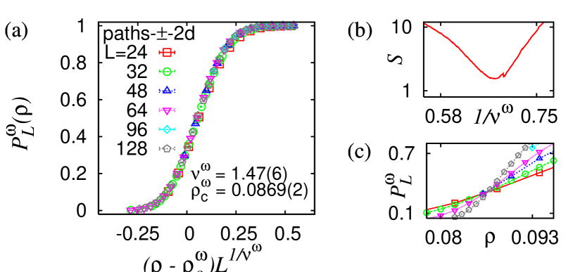
Within this problem, the aforementioned collection $\mathcal{C}$ consists of a set of loops, which might be empty, and a MWP spanning the lattice between the free boundaries. Since the MWP is anyway of $O(L)$ in the vertical direction by construction, we call the path percolating, if its projection on the horizontal axis (i.e. its roughness $r$) covers the full systems. We studied $2d$ lattices with $\pm$J disorder and sampled over up to $3.5\!\times\!10^{4}~{}(L\!=\!128)$ realizations of the disorder to perform averages, subsequently denoted by $\langle\ldots\rangle$. Firstly, we investigate the percolation probability. For a very small fraction $\rho$ of negative edge weights, the path will cross the lattice in a rather direct fashion, since overhangs are likely to increase the weight of the path and hence the weight of the whole configuration $\mathcal{C}$. Increasing $\rho$ also increases the spanning probability $P_{L}^{\rm{x}}(\rho)$, i.e. the probability of the horizontal extension to be $O(L)$. It is expected to scale as $P_{L}^{\rm{x}}(\rho)\!\sim\!f[(\rho-\rho_{c})L^{1/\nu}]$, where the critical exponent $\nu$ describes the divergence of the correlation length at the critical point $\rho_{c}$ and $f$ is a universal function. A data collapse, obtained using the method described in [9], yields $\rho_{c}$ and $\nu$ as listed in table 1 with a “quality” $S\!=\!0.79$ of the scaling assumption. We want to point out that the value of $\nu$ found here is clearly distinct from the value $4/3$ of conventional bond percolation, that would give a much worse quality of $S\!=\!5.20$ (see also figure 4(b)). Note that many negative weights are needed to allow the MWP to percolate. And indeed, the path weight becomes negative above $\rho_{c}^{\omega}\!=\!0.0869(2)$ with a probability that approaches unity quickly. Therein, the finite-size behavior is described by an exponent $\nu^{\omega}$ consistent with the value $\nu$ stated above, see figure 4.

Further note that $P_{L}^{\rm{x}}(\rho)\!<\!1$ even for large $\rho$, where the spanning probability seems to saturate slightly above $0.8$. The reason is, as already mentioned, that we actually do not optimize the length of a single path but the weight of the whole configuration $\mathcal{C}$. However, this behavior is clearly distinct from conventional percolation theory.

Next, we consider the probability $P_{L}^{\infty}\!\equiv\!\langle\ell\rangle/L^{d}$ that a bond belongs to the path, where $\langle\ell\rangle$ is the mean path length. It exhibits the finite-size scaling behavior $P_{L}^{\infty}(\rho)\!\sim\!L^{-\beta/\nu}f[(\rho-\rho_{c})L^{1/\nu}]$, where $\beta$ signifies the percolation strength [13]. Here, we fixed $\rho_{c}$ and $\nu$ as obtained above and determined the value of $\beta$ ($S\!=\!0.97$) listed in table 1. Adjusting all three parameters in the above scaling assumption yields $\rho_{c}\!=\!0.1027(1)$, $\nu\!=\!1.45(4)$ and $\beta\!=\!1.06(2)$ with a quality $S\!=\!0.76$. Note that the values agree within the errorbars.

We also determined some quantities (see also table 1) just at $\rho_{c}=0.1032(5)$ with additional simulations up to $L=512$ ($2\times 10^{3}$ samples). We studied the associated finite-size susceptibility $\chi_{L}\!=\!L^{-d}(\langle\ell^{2}\rangle\!-\!\langle\ell\rangle^{2})$. Its finite size-scaling at $\rho_{c}$ can be described using the exponent $\gamma$ via $\chi_{L}\!\sim\!L^{\gamma/\nu}$. Furthermore, the mean path length shows the critical behavior $\langle\ell\rangle\!\sim\!L^{d_{f}}$, where $d_{f}$ denotes the fractal exponent of the paths. Here, calculations at $\rho_{c}\!=\!0.1027(1)$ would result in a slightly smaller value of $d_{f}$. We further find the roughness exponent $d_{r}$ from $\langle r\rangle\!\sim\!L^{d_{r}}$ to be compatible with unity. Note that the obtained exponents satisfy the scaling relations $d_{f}\!=\!d\!-\!\beta/\nu$ and $\gamma\!+\!2\beta\!=\!d\nu$. We also measured the mean path weight $\langle\omega_{p}\rangle$ at the percolation point $\rho_{c}$ and found that $\langle\omega_{p}\rangle\!\sim\!\langle\ell\rangle$ for $L\!\rightarrow\!\infty$ seems to hold.

We can further probe $\mathcal{C}$ to not only investigate the MWP but to yield exponents that describe the small loops. A detailed study of the scaling behavior (length $\ell$ as function of the spanning length $R$, not shown here) at $\rho_{c}$ shows that they seem within error bars to exhibit the same fractal dimension $\tilde{d}_{f}\!=\!d_{f}$ as the MWPs. The loops also exhibit a mean (negative) weight that increases linearly with the loop length $\ell$. Further, one expects the distribution $n_{\ell}$ of loop lengths $\ell$ to exhibit an algebraic scaling $n_{\ell}\!\sim\!\ell^{-\tau}$, where $\tau$ signifies the Fisher exponent. Here, finite-size effects and the presence of the path lead to a suppression of large loops and thus to a deviation from the expected scaling behavior already for rather small values of $\ell$. In this question, we find a most reliable value $\tau$ if we account for corrections to scaling via $n_{\ell}\!\sim\!\ell^{-\tau}/(1+b\ell^{\omega})$, see table 1 and inset of figure 6. In principle, at criticality, the Fisher exponent and fractal dimension are related through the scaling relation $\tau\!-\!1\!=\!d/d_{f}$. This would lead us to expect $\tau\!\approx\!2.58$.

Finally, in $2d$ we can associate a cluster with each loop. The respective volume $v$ is measured as the number of enclosed plaquettes. It scales as $\langle v\rangle\!\sim\!R^{\tilde{d}_{v}}$ with $\tilde{d}_{v}=2.00(1)$, revealing the compact nature of the loops interior.

4 Minimal-weighted loop configurations

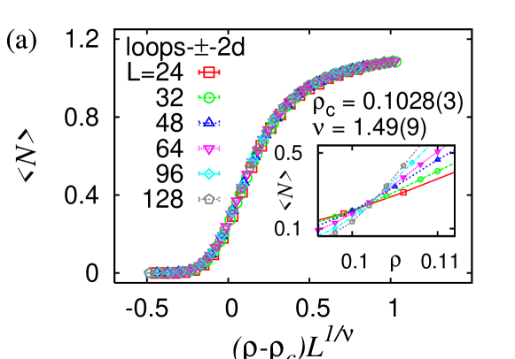
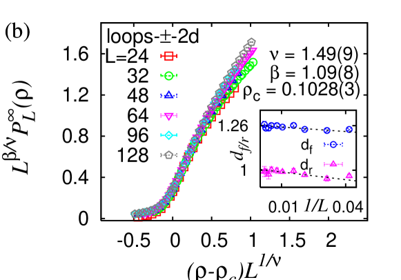
Here, we studied $2d$ (hex, $3d$) lattices with size up to $L\!=\!128$ ($192$, $48$) and $4.5\!\times\!10^{4}$ ($1.2\!\times\!10^{4}$, $1.6\!\times\!10^{4}$) samples. First, we analyze the largest loop for a given realization of the disorder. We find the linear extensions of the loops by projecting it onto all perpendicular axes. A loop is said to span the lattice, if its projection completely covers at least one axis. From the probability $P_{L}^{\rm{s}}(\rho)$ that a loop spans the lattice we estimate $\rho_{c}$ and $\nu$ listed in table 1. The qualities of the scaling law were found to be $S^{\pm}_{\rm{2d}}=1.09$, $S^{\pm}_{\rm{hex}}=0.79$, $S^{\rm{Gl}}_{\rm{2d}}=0.91$ and $S^{\pm}_{\rm{3d}}=1.9$. Further, it is interesting to note that the mean number of spanning loops $\langle N\rangle$ satisfies a similar scaling relation as the percolation probability, see figure 5(a), governed by the same values for $\rho_{c}$ and $\nu$ as $P_{L}^{\rm{s}}(\rho)$. In either case we find $\langle N\rangle\!>\!1$ for large values of $\rho$, as mentioned already in the introduction, see also [11]. As above, the probability $P_{L}^{\infty}(\rho)$ that an edge belongs to the percolating loop can be used to determine the exponent $\beta$, see figure 5(b) and table 1. Herein, the qualities of the scaling law were $S^{\pm}_{\rm{2d}}\!=\!1.88$, $S^{\pm}_{\rm{hex}}=0.32$, $S^{\rm{Gl}}_{\rm{2d}}\!=\!1.16$ and $S^{\pm}_{\rm{3d}}\!=\!2.08$. Interestingly, the values of $\rho_{c}$, $\nu$ and $\beta$ for the $2d$ loops with $\pm$J disorder are reasonable close to those of the $2d$ random-bond Ising model with $\rho_{c}\!=\!0.103(1)$, $\nu\!=\!1.55(1)$ and $\beta\!=\!0.9(1)$, see [3] and references therein. This probably means that the $2d$ ferromagnet to spin glass transition at $T\!=\!0$ can be explained in terms of a percolation transition in the following way: For a spin glass, one starts with a ferromagnetic configuration and searches for loops in the dual lattice with negative weight. These loops correspond to clusters of spins, which can be flipped to decrease the energy. If these loops are small, i.e. not percolating, the ground state is ferromagnetic, otherwise the ground state exhibits spin-glass order. A different argument relating this transition to a percolation transition was also briefly mentioned in a study, which focuses on the critical slowing down of polynomial-time algorithms at $T\!=\!0$ phase transitions [17].

Right at $\rho_{c}$ we studied $2d$ (hex, $3d$) systems up to $L\!=\!512$ ($768$, $96$) with $3.2\!\times\!10^{4}$ ($1.6\!\times\!10^{3}$, $6.4\!\times\!10^{3}$) samples. For the $2d$ systems we found $\gamma$ listed in table 1 with qualities $Q^{\pm}_{\rm 2d}\!=\!0.61$, $Q^{\pm}_{{\rm hex}}\!=\!0.10$ and $Q^{\rm{Gl}}_{\rm 2d}\!=\!0.51$. In $3d$, due to the very small percolation probability $0.0014(1)$ at $\rho_{c}$ our results are less clear. Hence, we can draw no final conclusions for that case. Regarding the fractal dimension, spanning loops and the non-spanning loops exhibit within error bars the same exponents $d_{f}=\tilde{d}_{f}$ in $2d$ (values of $d_{f}$ listed in table 1). As in the MWP case, the non-spanning loops are compact ($\langle v\rangle\!\sim\!R^{2}$). On the other hand, in $3d$, we find $\tilde{d}_{f}=1.43(2)$ different from $d_{f}=1.30(1)$.

Also regarding the mean weight $\langle\omega_{\ell}\rangle$ for given length $\ell$, we find in $2d$ that spanning and non-spanning loops exhibit both $\langle\omega_{\ell}\rangle\!\sim\!\ell$ (i.e. $\sim L^{d_{f}}$ for the spanning loops), while in $3d$ the quality of the data is again not sufficient to observe a clear power law.

Figure 6: Results for the $2d$ $\pm$J loops: distribution $n_{\ell}$ of the loop-lengths $\ell$ at criticality, excluding the spanning loops (main plot), gray data points were omitted from the fit. The inset shows $n_{\ell}$ for the case of MWPs, where the fit accounts for corrections to scaling (see text).

Figure 7: Performance of the algorithm for $2d$ Gl loops: the main plot shows the average number of dual adjustments per site for different system sizes $L$ and the inset illustrates the associated finite-size susceptibility.

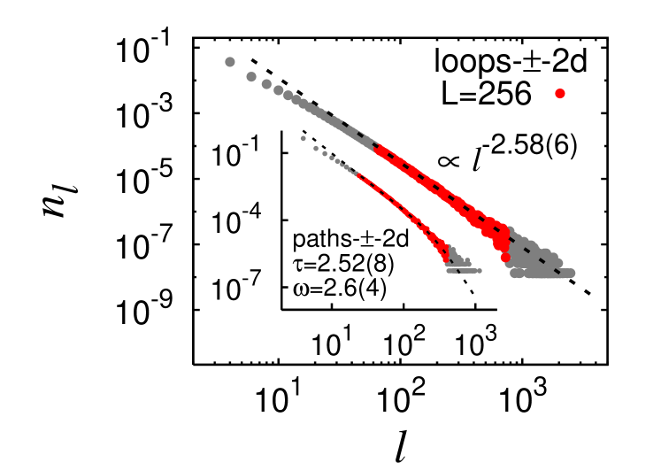
The distribution of loop-lengths, excluding the truly spanning loops, is in $2d$ in good agreement with a power-law decay $n_{\ell}\!\sim\!\ell^{-\tau}$, see figure 6 and table 1. In $3d$ we find again strong finite size effects and hence a most reliable estimate of $\tau$ using a scaling form $n_{\ell}\!\sim\!\ell^{-\tau}/(1+b\ell^{\omega})$ .

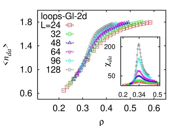
Finally, we address the performance of the algorithm. We doe not want to measure the running time in terms of CPU minutes, since this is machine dependent and is also influenced by external factors like which other processes are running. Hence, we have to look at the algorithm more closely. So as to determine a minimum-weight perfect matching, the algorithm attempts to find an optimal solution to an associated dual problem [6, 8]. Therein, the basic task of the algorithm is to find augmenting paths that improve the solution to the latter. While executing, the solution to the dual problem is adjusted several times. As a measure for the algorithm performance we consider the number $N_{da}$ of such adjustment operations, until the algorithm terminates. Figure 7 shows the average number of these operations per lattice site $\langle n_{da}\rangle\!=\!L^{-d}\langle N_{da}\rangle$ for the case of a Gaussian-like distribution of the edge weights. The value of $\langle n_{da}\rangle$ increases with increasing $\rho$ and curves for different system sizes deviate from each other as the critical point is approached from below. At $\rho_{c}$ it scales like $\langle n_{da}\rangle\!\sim\!L^{2.074(4)}$. Moreover, the corresponding susceptibility $\chi_{da}$, i.e. the fluctuations of the $n_{da}$, diverges at the critical point where is scales as $\chi_{da}\!\sim\!L^{1.41(4)}$, as can be seen from the inset of figure 7. For the case of a $\pm$J distribution of the edge weights, we found similar but slightly different results (not depicted): Here, data sets that describe the scaling of $\langle n_{da}\rangle$ for different system sizes, fall onto one universal curve everywhere. This holds also for $\chi_{da}$, which is peaked slightly below the critical point at $\rho\!\approx\!0.096$.

5 Conclusions

We have introduced a percolation problem, where edge weights with possibly negative values are attached to the edges. A system is called percolating if spanning loops or paths of negative weight exist. Hence, this model might be fundamentally different from classical percolation problems. We studied systems in $2d$ and $3d$ up to large system sizes. In all cases, the universality class is indeed clearly different from standard bond/site percolation. Further, the values of the fractal exponents obtained for the paths/loops differ from those reported in the context of shortest paths or hulls of percolation clusters, so far. Nevertheless, the numerical values for the exponents found here are close to those of disorder-induced single defects ($d_{f}\!=\!1.261(16)$) and multiple defects ($d_{f}\!=\!1.250(3)$) in a $2d$ elastic medium at zero temperature [16]. We observe universality in $2d$, hence the properties are independent of the type of weight distribution, lattice geometry and the same for loops or paths. We also studied (not shown here) a related problem, where the loops are allowed to intersect. The corresponding mapping was recently used in a different context to determine extended ground states of Ising spin glasses [15]. We found again the same critical exponents. On the other hand, we observe in $2d$ the same behavior as for the $T\!=\!0$ ferromagnet to spin glass transition for the random-bond Ising model, hence this physical transition can be probably explained by a percolation transition in the spirit of the model we have introduced here. Hence, studying percolation problems with negative weights and similar generalizations might be a key approach to describe many yet not well-understood phase transitions in terms of percolation transitions. We also anticipate applications to other fields like social problems (see introduction) or other types of networks.

References

- [1] For the calculation of minimum-weighted perfect matchings we use Cook and Rohes blossom4 extension to the Concorde library http://www2.isye.gatech.edu/~wcook/blossom4/
- [2] Ahuja R K, Magnanti T L and Orlin J B 1993 Network Flows: Theory, Algorithms and Applications (New Jersey: Prentice Hall)
- [3] Amoruso C and Hartmann A K 2004 Phys. Rev. B 70 134425
- [4] Antunes N D and Bettencourt L M A 1998 Phys. Rev. Lett. 81 3083–86
- [5] Bittner E, Krinner A and Janke W 2005 Phys. Rev. B 72 094511
- [6] Cook W and Rohe A 1999 INFORMS J. Computing 11 138–48
- [7] Engels J, Mashkevich S, Scheideler T and Zinovjev G 1996 Phys. Lett. B 365 219
- [8] Hartmann A K and Rieger H 2001 Optimization Algorithms in Physics (Berlin: Wiley-VCH)
- [9] Houdayer J and Hartmann A K 2004 Phys. Rev. B 70 014418 measures the mean square distance of the scaled data to the master curve in units of standart errors
- [10] Melchert O and Hartmann A K 2007 Phys. Rev. B 76 174411
- [11] Pfeiffer F O and Rieger H 2003 Phys. Rev. E 67 056113
- [12] Schakel A M J 2001 Phys. Rev. E 63 026115
- [13] Stauffer D and Aharony A 1994 Introduction to Percolation Theory (London: Taylor and Francis)
- [14] Wenzel S, Bittner E, Janke W, Schakel A M J and Schiller A 2005 Phys. Rev. Lett. 95 051601
- [15] Thomas C K and Middleton A A 2007 Matching Kasteleyn cities for spin glass ground states arXiv:0706.2866
- [16] Middleton A A 2000 Phys. Rev. B 61 14787
- [17] Middleton A A 2002 Phys. Rev. Lett. 88 017202