Perturbations of the signum-Gordon model

Abstract

We investigate a perturbation of a scalar field model (called here the signum-Gordon model) with the potential $V(f)=|f|$. The perturbation generalizes the signum-Gordon model to the signum-Klein-Gordon model i.e. to the case $V(f)=|f|-\frac{1}{2}\lambda f^{2}$, where $\lambda$ is a small parameter. Such a generalization breaks the scaling symmetry of the signum-Gordon model. In this paper we concentrate on solutions for self-similar initial data. Such data are particulary useful for identification of the effects caused by the term that breaks the scaling symmetry. We have found that the behaviour of the solutions is quite interesting - they escape and return periodically to the self-similar initial data.

PACS: 05.45.-a, 03.50.Kk, 11.10.Lm
Preprint TPJU - 15/2006

1 Introduction

The present paper refers to recently investigated scalar field models with V-shaped potential [1]-[3]. Such potentials have a common feature - left- and right hand derivatives are different from zero at the minimum. Mentioned models have a well-justified physical origin despite the fact that they seem to be a little bit exotic from a mathematical viewpoint. Moreover, some physical systems described by scalar field models with V-shaped potentials are easy to built (e.g. chain of pendulums impacting on a rectilinear bar). Unfortunately, such models have a very unpleasant mathematical feature - a typical solution consists of many (sometimes infinitely many) partial solutions. The partial solutions are matched at some points. The matching procedure is mostly onerous. This is probably the reason why literature is poor in results for field theoretic models with V-shaped potential.

It turns out that the behaviour of the field close to minimum strongly depends on a ’shape’ of the potential [4]. In particular, for V-shaped potential a field approaches exactly its vacuum value at finite distance (a parabolic approach). This fact has a profound significance - kinks have no exponential tails! Such kinks are called compactons because their supports are compact. The compactons considered in our models are topological, so they are qualitatively different from e.g. well-known compactons in the modified KdV model [5]-[7]. Recently, the topological compactons have been also obtained in models with nonstandard kinetic terms as so-called $k$-defects [8]. It is important to notice that there are other (nontopological) compact solutions in the s-G model [9]. Because of their properties they are called oscillons.

The second characteristic property of the mentioned models is a scaling symmetry, see [2]. This symmetry means that if a function $f(x,t)$ is a solution of a field equation, then new function defined as $f_{\nu}(x,t)=\nu^{2}f(x/\nu,t/\nu)$ is a solution as well. $\nu$ is here a positive constant. A presence of the scaling symmetry in the model suggests existence of solutions that are invariant with respect to the scaling transformation (so-called self-similar solutions). Such solutions have been obtained in the s-G model. A complete list of solutions for the self-similar initial data is presented in [10]. For models with the potential $V(f)=af\Theta(-f)+bf\Theta(f)$, where $a$, $b$ are constant parameters and $\Theta$ is the well-known Heaviside step function, the scaling symmetry is exact whereas for most models with V-shaped potential the symmetry is only approximated. Note that the signum-Gordon model (s-G) can be obtained as a particular case, i.e. by setting $a=-1$ and $b=1$. In a group of models with symmetric V-shaped potential, the s-G model is the simplest one. In this paper we study just symmetric potentials.

The aim of the present work is the analysis of the perturbed s-G model, where for simplicity reasons the specific perturbation is chosen in the simplest, nontrivial form. Namely, we add the quadratic term. In spite of its simplicity such a generalization of the s-G model allows to face several important problems. The first one is breaking of the scaling symmetry. Among the physical systems there are fewer of them with an exact scaling symmetry. There are always fluctuations in a typical physical system that interacts with its environment. The fluctuations modify an effective potential and break the exact scaling symmetry. In this physical context, it is clear that investigation of the perturbed field theoretic models with V-shaped potentials is an important issue. It allows for better understanding of dynamics of compactons in the systems with the broken scaling symmetry. In our paper we analyse the perturbed potential $V(f)=|f|-\frac{1}{2}\lambda f^{2}$, where $\lambda$ is a small parameter i.e. $|\lambda|\ll 1$. The second important problem, which is in general very difficult for systems with non-differentiable potentials, is a stability analysis of solutions. Our investigations are some kind of structural stability analysis. Such analysis is important for compact kinks as well as compact oscillons.

However, the models with V-shaped potentials are interesiting from the mathematical point of view, they have also some properties that allow to think about possible applications to condense matter physics and cosmology as well. In the cosmological context, the most interesiting seems to be the fact that for models with potentials sharp at its minima the terms that come from a gradient of the potential dominate the field dynamics close to the minimum. For instance, in the s-G model the term $\frac{dV}{df}=\hbox{sign}f$ remains finite arbitrary close to the minimum. This is in total oposition to the behaviour of e.g. $\phi^{4}$ theory, where gradient of the potential vanishes close to the minimum. Because of this, small perturbations propagate easily within the topological compactons or other nontopological field configurations like, e.g. mentioned oscillons, whereas outside of them the propagation encounters on resistance. Moreover, an absence of linear perturbations around the V-shaped minimum is a basic feature of our models. It entails automatically that the linear perturbations can propagate only at a defect background. This effect, characteriscic for models with V-shaped potentials, is similar to behaviour of $k$-fields that play a prominent role in cosmology (see [11]).

In our calculation we concentrate on differences between solutions in the s-G model and solutions in the signum-Klein-Gordon (s-K-G) model (the perturbed model). Applying the same initial data for solutions in both these models we can analyse the differences between their solutions as a pure effect caused by the term $\frac{1}{2}\lambda f^{2}$. In the case when initial data are self-similar (parabolic) the solutions in the s-G model have especially simple form. We apply the self-similar data just for this reason.

Our paper is organized as follows. In the section 2 we introduce the signum-Klein-Gordon (s-K-G) model and give a general method of calculation of partial solutions that can be obtained directly from the self-similar initial data. Unfortunately, they are insufficient to construct a solution valid for each $x$ and $t>t_{0}$, where $t_{0}$ is an initial moment. Section 3 is devoted to a study of a solution for a specific self-similar initial data. Focusing on a specific initial data enables us to calculate all partial solutions that (when matched together) cover the whole range of variable $x$. In the last section we summarize our results and emphasize effects that stem from the term $\frac{1}{2}\lambda f^{2}$.

2 Initial problem for the generalized model

2.1 The signum-Klein-Gordon model and its partial solutions

The s-K-G model for the scalar field $f(x,t)$ in 1+1 dimensions has the Lagrangian

$$L=\frac{1}{2}(\partial_{t}f)^{2}-\frac{1}{2}(\partial_{x}f)^{2}-V(f),$$ (1)

where the potential $V(f)$ is given by the formula

$$V(f)=|f|-\frac{1}{2}\lambda f^{2}.$$ (2)

Euler-Lagrange equation that corresponds to Lagrangian (1) takes the following form

$$(\partial^{2}_{t}-\partial^{2}_{x})f+\hbox{sign}f-\lambda f=0.$$ (3)

The sign of parameter $\lambda$ has a crucial meaning for the behaviour of the field $f(x,t)$. The potentials $V(f)$ for negative and positive values of parameter $\lambda$ are qualitatively different [3]. The case $\lambda=0$ gives the s-G model which has been discussed in our previous papers, (see e.g. [1], [2] and [10]). In this paper we are interested in the case $\lambda<0$, because for $\lambda>0$ the potential $V(f)$ is not bounded from below. Nevertheless, a perturbative method presented in the following subsection involves both cases of sign $\lambda$. In order to distinguish between different kind of solutions, we use symbol $f$ for solutions in the s-K-G model ($\lambda\neq 0$) and symbol $\phi$ for solutions in the s-G model. The partial self-similar solutions are given by the formula

$$\phi_{k}(x,t)=\frac{(-1)^{k}}{2}\frac{(x-v_{k-1}t)(x-v_{k}t)}{v_{k-1}v_{k}-1},$$ (4)

where $x\in[v_{k-1}t,v_{k}t]$ and $k=1,2,\ldots$. The parameters $v_{k}$ are velocities of zeros of polynomials. They are determined from matching conditions. For more details see [10]. The partial solutions obey the relation $\hbox{sign}\phi_{k}=(-1)^{k+1}$. By analogy, we define partial solutions in the model with $\lambda\neq 0$. They obey the equation

$$(\partial^{2}_{t}-\partial^{2}_{x})f_{k}(x,t)-(-1)^{k}-\lambda f_{k}(x,t)=0,$$ (5)

where $\hbox{sign}f_{k}=(-1)^{k+1}$. For $|\lambda|\ll 1$ the potential $V(f)=|f|-\frac{1}{2}\lambda f^{2}$ can be interpreted as a perturbed potential $V(\phi)=|\phi|$. In this case we say that the exact scaling symmetry is violated or that the generalized model has an approximate scaling symmetry when $|f|\gg\lambda f^{2}$.

2.2 Self-similar initial data and partial solutions

This paper is devoted to investigation which are the effects caused by the term $\lambda f$ in the s-K-G equation. It can be achieved by comparison two solutions for the same initial data: the first one that is a solution in the s-G model and the second one that comes from the s-K-G model. The differences between them are a direct consequence of the term that breaks the scaling symmetry. From practical reasons we investigate some characteristic points of solutions, i.e. trajectories of its zeros.

It turns out that explicit formulae for the solutions are not always available - this problem strongly depends on initial data. It has been shown, see [10], that solutions in the s-G model for the self-similar (parabolic) initial data are given by explicit formulae. For this reason, the self-similar initial data are more useful for our purposes than other, more general, initial data. In fact, any self-similar solution $\phi$ at the moment $t=t_{0}$ is suitable for our purposes and can be applied as an initial data. Therefore, we assume following initial data for the partial solutions

$$f_{k}(x,t_{0})=\phi_{k}(x,t_{0}),\qquad\partial_{t}f_{k}(x,t)|_{t=t_{0}}=\partial_{t}\phi_{k}(x,t)|_{t=t_{0}}.$$ (6)

2.3 The perturbative method

The method presented in the current subsection allows us to obtain the partial solutions $f_{k}(x,t)$ directly from the initial data (6). We call them the partial solutions of the first kind. It turns out that such partial solutions are insufficient. A complete solution $f(x,t)$ is consisted of some other partial solutions as well. This inconvenience appears also for, e.g. the s-G equation in the case when initial data have the form of piecewise smooth functions matched up at some points. In most cases, such matching points are origins of new partial solutions. At the initial moment $t=t_{0}$ mentioned partial solutions are shrunk to single points but for $t>t_{0}$ their supports expand (the partial solutions of the second kind). The s-K-G model has analogical partial solutions (the first and the second kind) - we discuss their properties in the further part of this paper. The partial solutions discussed in this paragraph are the first kind ones. They cover whole range of axis $x$ at $t=t_{0}$ (they obey (6) where $\phi_{k}$ have this property) and their supports shrink for $t>t_{0}$.

Let us assume that the solutions $f_{k}(x,t)$, which depend on parameter $\lambda$, are represented in the form of a power series

$$f_{k}(x,t)=\sum_{n=0}^{\infty}f_{kn}(x,t)\lambda^{n},$$ (7)

where $\lambda\ll 1$. After plugging series (7) into equation (5) we get a set of equations

$$\left\{\begin{array}[]{ll}(\partial^{2}_{t}-\partial^{2}_{x})f_{k0}(x,t)=(-1)^{k}&n=0,\\ (\partial^{2}_{t}-\partial^{2}_{x})f_{kn}(x,t)=f_{kn-1}(x,t)&n=1,2,3,\ldots.\end{array}\right.$$ (10)

Each of them takes the form of wave equation with a source. We can integrate them using new variables $\xi=\frac{1}{2}(x+t)$, $\eta=\frac{1}{2}(x-t)$. The result of integration in the original variables reads

$$f_{k0}(x,t)=F_{0}(x+t)+G_{0}(x-t)-\frac{(-1)^{k}}{4}(x^{2}-t^{2}),$$ (11)

$$f_{kn}(x,t) = F_{n}(x+t)+G_{n}(x-t)-\int_{0}^{\frac{x+t}{2}}\hbox{d}\alpha\int_{0}^{\frac{x-t}{2}}\hbox{d}\beta\;f_{kn-1}(\alpha+\beta,\alpha-\beta),$$

where $F(x+t)$ and $G(x-t)$ are arbitrary functions. They can be calculated from the following initial conditions for the partial solutions:

$$f_{k0}(x,t_{0})=\phi_{k}(x,t_{0}),\qquad\partial_{t}f_{k0}(x,t)|_{t=t_{0}}=\partial_{t}\phi_{k}(x,t)|_{t=t_{0}},$$ (13)

$$f_{kn}(x,t_{0})=0,\qquad\partial_{t}f_{kn}(x,t)|_{t=t_{0}}=0.$$ (14)

Conditions (13) and (14) stem from the initial conditions (6). The solution (11) obeys the first of the equations (10) (i.e. the s-G equation) and the self-similar initial data (13), so it coincides with $\phi_{k}$,

$$f_{k0}(x,t)=\phi_{k}(x,t).$$ (15)

A direct calculation confirms this result. It means that the self-similar solutions (15) are zero-order approximation for the solutions (7). In order to get higher-order approximations we have to find the functions $F_{n}(x+t)$ and $G_{n}(x-t)$. Differentiating first of equations (14) with respect to $x$, combining with the second one and shifting arguments, we obtain equations

$$D_{+}f_{kn}(x,t)\left.\right|_{x=s-t_{0},\;t=t_{0}}=0,\qquad D_{-}f_{kn}(x,t)\left.\right|_{x=w+t_{0},\;t=t_{0}}=0,$$ (16)

where $D_{\pm}\equiv\frac{1}{2}(\partial_{x}\pm\partial_{t})$. Equations (16) can be rewritten in the form

$$F^{\prime}_{n}(s)=\left.D_{+}\int_{0}^{\frac{x+t}{2}}\hbox{d}\alpha\int_{0}^{\frac{x-t}{2}}\hbox{d}\beta\;f_{kn-1}(\alpha+\beta,\alpha-\beta)\right|_{x=s-t_{0},\;t=t_{0}},$$ (17)

$$G^{\prime}_{n}(w)=\left.D_{-}\int_{0}^{\frac{x+t}{2}}\hbox{d}\alpha\int_{0}^{\frac{x-t}{2}}\hbox{d}\beta\;f_{kn-1}(\alpha+\beta,\alpha-\beta)\right|_{x=w+t_{0},\;t=t_{0}},$$ (18)

where formula (2.3) has been applied. The sum of constants that comes from integration of the expressions (17) and (18) is fixed by the first of conditions (14).

In the first step we calculate the function $f_{k1}(x,t)$ from formula (2.3). Then we can continue the procedure in order to obtain $f_{k2}(x,t)$. In principle, this procedure can be repeated infinitely many times giving expressions for all functions $f_{kn}(x,t)$. In fact, we are able to obtain only few functions $f_{kn}(x,t)$ because the calculations became quickly too complicated. Fortunately, functions $f_{kn}(x,t)$ obtained for several, the lowest values of $n$ enable us to guess a general formula for arbitrary $n$. This formula has the form

$$f_{kn}(x,t)=(-1)^{k}\frac{(t-t_{0})^{2n}}{(2n+2)!}\frac{A_{n}x^{2}+B_{n}x+C_{n}}{v_{k-1}v_{k}-1},$$ (19)

where

$$A_{n}=(2n+1)(n+1),$$

$$B_{n}=-(v_{k-1}+v_{k})(n+1)(t+2nt_{0}),$$

$$C_{n}=(n+v_{k-1}v_{k})t^{2}+n(1+(2n+1)v_{k-1}v_{k})t_{0}^{2}.$$

One can check that formula (19), which was originally found for $n=1,2,\ldots$, is also true for $n=0$ - in this case it gives (15).

It turns out, and this is a big surprise, that the series (7) can be summed up giving as a result

$$f_{k}(x,t) = \frac{(-1)^{k}}{2(v_{k-1}v_{k}-1)}\left[M\cosh{(\rho(t-t_{0}))}+N\frac{\sinh{(\rho(t-t_{0}))}}{\rho}\right]+$$ (20)

$$+ \frac{(-1)^{k}}{\rho^{2}}[\cosh{(\rho(t-t_{0}))}-1],$$

for $\lambda\equiv\rho^{2}>0$, and

$$f_{k}(x,t) = \frac{(-1)^{k}}{2(v_{k-1}v_{k}-1)}\left[M\cos{(\sigma(t-t_{0}))}+N\frac{\sin{(\sigma(t-t_{0}))}}{\sigma}\right]+$$ (21)

$$+ \frac{(-1)^{k}}{\sigma^{2}}[1-\cos{(\sigma(t-t_{0}))}],$$

for $\lambda\equiv-\sigma^{2}<0$. The coefficients $M$ and $N$ read

$$M\equiv(x-v_{k-1}t_{0})(x-v_{k}t_{0}),$$

$$N\equiv t-t_{0}+2v_{k-1}v_{k}t_{0}-(v_{k-1}+v_{k})x.$$

The partial solutions $f_{k}$ satisfy the relation $\hbox{sign}f_{k}=(-1)^{k+1}$.

It is worth emphasizing that the partial solutions $f_{k}$ in the model with the explicitly broken scaling symmetry, still have a quadratic dependence on variable $x$. What changes is the time dependence. This is the first important result obtained with the help of the perturbative method.

Knowing this result we can, of course, propose a posteriori a proper Ansatz

$$f_{k}(x,t)=a(t)x^{2}+b(t)x+c(t).$$ (22)

Plugging the Ansatz (22) into eq. (5) we get the set of ordinary differential equations for the coefficients $a(t)$, $b(t)$ and $c(t)$

$$\frac{d^{2}a}{dt^{2}}-\lambda a=0,\qquad\frac{d^{2}b}{dt^{2}}-\lambda b=0,\qquad\frac{d^{2}c}{dt^{2}}-\lambda c=2a+(-1)^{k}.$$

The constants that come from integration of these equations are fixed by the condition (6). Solving these equations we recover formulae (20) and (21) depending on sign of the parameter $\lambda$.

3 The solution for a specific initial data

In this section we present a solution in the s-K-G model for a specific self-similar initial data. We concentrate on the case when the perturbative parameter $\lambda$ is small $|\lambda|\ll 1$ and negative $\lambda=-\sigma^{2}$. The main effort is focused on the partial solutions of the second kind. They can be obtained as the solutions of boundary problem. The boundary conditions are given by the partial solutions of the first kind at points of contact of their supports and supports of the partial solutions of the second kind. The most serious obstacle in the s-K-G model is that we do not know a general formula for the partial solutions. For instance, in the s-G model such formula consists of two arbitrary functions and terms $\pm t^{2}/2$, $\pm x^{2}/2$ or their combinations. For this reason, we restrict our study to a specific self-similar initial data and construct an approximated solution. Nevertheless, it turns out that investigation of such a specified case gives valuable information as well. One of the most interesting results presented in the current section is a discovery of periodicity in time for such solution in the s-K-G model.

3.1 The positive partial solution $f_{+}(x,t)$

Among the self-similar initial data, the simplest one reads

$$\phi(x,0)=\frac{1}{4}x^{2}\Theta(x),\qquad\partial_{t}\phi(x,t)|_{t=0}=0,$$ (23)

where $\Theta(x)$ is the Heaviside step function. The self-similar solution $\phi(x,t)$ in the s-G model for data (23) is consisted of two partial solutions matched up at the light cone $x=t$, see also [10]. The solution $\phi(x,t)$ has a very simple form

$$\phi(x,t)=\frac{1}{4}(x^{2}-t^{2})\Theta(x-t).$$ (24)

This formula corresponds to (4) for $k=1$, $v_{0}=-1$ and $v_{1}=1$. The snapshot of the solution $\phi(x,t)$ is presented in Fig.1.

Figure 1: The self-similar solution for initial data (23). The dashed line represents an initial configuration of the field $\phi$.

In the further part of this paper we concentrate on the solution $f(x,t)$ in the s-K-G model. The positive partial solution $f_{+}(x,t)$ obeys the equation

$$(\partial^{2}_{t}-\partial^{2}_{x})f_{+}+\sigma^{2}f_{+}+1=0,$$ (25)

and the initial conditions

$$f_{+}(x,0)=\frac{1}{4}x^{2},\qquad\partial_{t}f_{+}(x,t)|_{t=0}=0.$$

It takes the form

$$f_{+}(x,t)=\frac{1}{4}\cos(\sigma t)x^{2}+\frac{t}{4\sigma}\sin(\sigma t)-\frac{1}{\sigma^{2}}(1-\cos(\sigma t)).$$ (26)

The partial solution (26) can be obtained directly from (21) for $k=1$ and $t_{0}=0$. The formula (26) holds for $x\geq x_{1}(t)$. The trajectory of zero $x_{1}(t)$,

$$x_{1}(t)=\frac{2}{\sigma}\sqrt{\frac{1}{\cos(\sigma t)}-\frac{\sigma t}{4}\tan(\sigma t)-1}$$ (27)

is the solution of the equation $f_{+}(x_{1},t)=0$. Except for the point $t=0$, the function $x_{1}(t)$ obeys inequality $x_{1}(t)>t$, what means that zero of $f_{+}(x,t)$ moves faster than its counterpart ($x(t)=t$) in the s-G model. Moreover, we can see that the velocity of zero $x_{1}(t)$ depends on variable $t$. Let us remind that velocities $v_{k}$ of zeros of the self-similar solutions are constant, see formula (4). It means that the term $\lambda f$ in the eq. (3) is responsible for non monotonous expansion or contraction of the supports of the partial solutions.

Figure 2: The trajectory $x_{1}(t)$ for $\lambda=-0.1$.

A series expansion of the formula (27) for small $t$

$$x_{1}(t)=t+\frac{1}{4}t^{3}\sigma^{2}+\frac{103}{1440}t^{5}\sigma^{4}+O(t^{7})$$ (28)

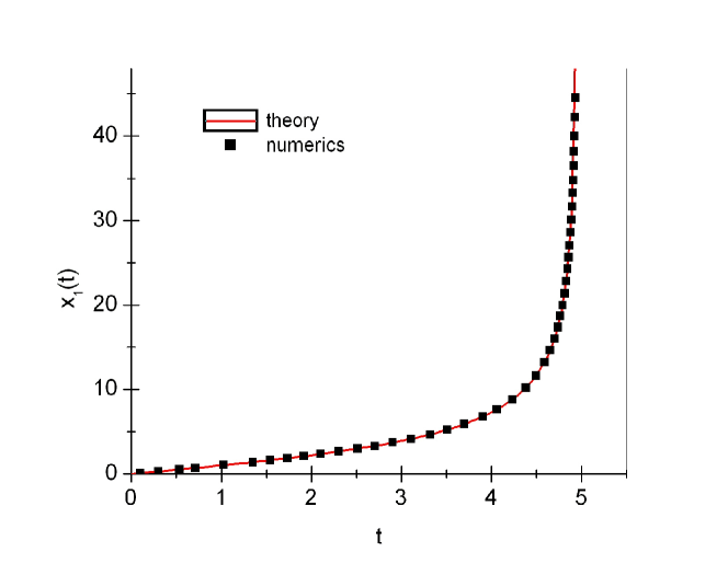
gives valuable information as well. We can see from (28) that the zero $x_{1}(t)$ moves with the acceleration $\ddot{x}_{1}(t)$ which is proportional to $\sigma^{2}$ provided that $t\ll 1$. This observation has a practical meaning because it enables us to calculate the parameter $\lambda$ from experimental data. The curve $x_{1}(t)$ is presented in the Fig. 2. We can see a very good agreement between the analytical calculation and the numerical data. The function (27) goes to infinity for $t\rightarrow t^{*}\equiv\frac{\pi}{2\sigma}$. It means that the solution $f_{+}(x,t)$ is valid for $t<t^{*}$. In our numerical calculation ($\sigma^{2}=0.1$) the characteristic time $t^{*}\approx 4.9673$. The leading behaviour of $x_{1}(t)$ close to $t^{*}$ is given by the first term of the expansion

$$x_{1}(t)=\frac{1}{2\sigma^{3/2}}\sqrt{\frac{16-2\pi}{t^{*}-t}}-\frac{3}{\sigma^{1/2}}\sqrt{\frac{t^{*}-t}{16-2\pi}}+O(\sigma^{1/2}).$$

3.2 The negative partial solution $f_{-}(x,t)$ - some general remarks

In this and two further paragraphes we present the partial solution of the second kind $f_{-}(x,t)$. Our solution is only approximated and holds for times not longer than $t\approx 2$. Such a partial solution can be obtained as the solution of boundary problem because at the initial time $t=0$ its support is a single point and it is located at $x=0$. For later times $t>0$ the support expands to infinite size. This behaviour has been observed in our numerical calculation and it is suggested by the fact that $x_{1}(t)$ tends to infinity for $t\rightarrow\frac{\pi}{2\sigma}$. The solution $f_{-}(x,t)$ has to obey the following boundary conditions

$$f_{-}(x_{1},t)=0,\qquad\partial_{x}f_{-}(x,t)|_{x=x_{1}}=\partial_{x}f_{+}(x,t)|_{x=x_{1}},$$ (29)

$$f_{-}(x_{0},t)=0,\qquad\partial_{x}f_{-}(x,t)|_{x=x_{0}}=0.$$ (30)

Conditions (29) and (30) are derived from the field equation (3) and they mean that the partial solutions are matched so that the solution $f(x,t)$ is smooth at $x_{1}(t)$ and $x_{0}(t)$. At $x_{0}(t)$ the partial solution $f_{-}(x,t)$ is matched with the trivial partial solution $f_{0}(x,t)=0$. Whereas the point $x_{1}(t)$ is given by the formula (27), the second zero of $f(x,t)$, i.e $x_{0}(t)$, is not known yet. In Section 3.4 we show how to obtain an approximated formula for $x_{0}(t)$.

Figure 3: The solution $f(x,t)$ for initial data (23) and times $t<\frac{\pi}{2\sigma}$ The dashed line represents an initial configuration of the field $f$.

It turns out that the partial solution that obeys (29) does not obey (30) and vice versa. In order to get rid of this inconvenience we split the solution $f_{-}(x,t)$ into two pieces $f_{-}^{L}(x,t)$ and $f_{-}^{R}(x,t)$. They are matched at the light cone $x=t$. Such split is sufficient to obtain $f_{-}(x,t)$ that obeys (29) and (30) simultaneously. The solution $f(x,t)$ consists of the following partial solutions

$$f(x,t)=\left\{\begin{array}[]{ll}0&\hbox{for}\quad x\leq x_{0}(t),\\ f_{-}^{L}(x,t)&\hbox{for}\quad x_{0}(t)\leq x\leq t,\\ f_{-}^{R}(x,t)&\hbox{for}\quad t\leq x\leq x_{1}(t),\\ f_{+}(x,t)&\hbox{for}\quad x\geq x_{1}(t),\end{array}\right.$$

where $t<\frac{\pi}{2\sigma}$. The snapshot of $f(x,t)$ is depicted in Fig. 3 - compare it to the solution in Fig. 1.

3.3 The partial solution $f_{-}^{R}(x,t)$

It has been already mentioned at the begining of Section 3 that a general formula for the partial solutions in the s-K-G model is not known. This is the most serious obstacle in our investigations. Therefore, we search for the approximated partial solution $f_{-}(x,t)$. The approximation of eq. (3) is obtained by replacing the term $\sigma^{2}f(x,t)$ by the term $\sigma^{2}\phi(x,t)$, what gives us

$$(\partial^{2}_{t}-\partial^{2}_{x})f_{-}(x,t)+\sigma^{2}\phi(x,t)-1=0.$$ (31)

Such a modification is valid only for small times. The partial solution $f_{-}^{R}(x,t)$ of eq. (31) (an approximate solution of eq. (3) for $\lambda=-\sigma^{2}$) at $t\leq x\leq x_{1}(t)$ has the form

$$f_{-}^{R}(x,t)=F_{R}(x+t)+G_{R}(x-t)-\frac{1}{4}(x^{2}-t^{2})+\frac{\sigma^{2}}{64}(x^{2}-t^{2})^{2}.$$ (32)

In accordance with (29), this solution is matched to $f_{+}(x,t)$ at $x=x_{1}(t)$. It turns out that exact formulas for $F_{R}(x+t)$ and $G_{R}(x-t)$ can not be achieved because we need the inverse functions of $x_{1}(t)\pm t$, where $x_{1}(t)$ is given by (27). Nevertheless, we can expand the expressions $x_{1}(t)\pm t$ in power series and then invert these series up to an arbitrary term. This is why we concentrate on series expansions of the partial solutions. In our further calculations we use the perturbation parameter $\sigma$ as an expansion parameter. The partial solutions represented by finite series (i.e. approximated partial solutions) obey the matching conditions (29) and (30) up to some range of $\sigma$. In order to find this range we start from series expansion of the formula (27) for $\sigma\ll 1$, i.e.,

$$x_{1}(t)=t+\frac{1}{4}t^{3}\sigma^{2}+\frac{103}{1440}t^{5}\sigma^{4}+O(\sigma^{6}).$$ (33)

Note that the expansion (33) has the same form as the expansion (28) for small times $t$. A leading term of the expression $x_{1}(t)-t$ is proportional to $\sigma^{2}$. The powers of the expression $x_{1}(t)-t$ appear in (29) because the partial solution $f_{-}^{R}(x,t)$, which is given by formula (32), includes terms proportional to $x-t$ and $\sigma^{2}(x-t)^{2}$. In order to take into consideration contributions from all terms in (32), especially from $\sigma^{2}(x-t)^{2}$, we need terms proportional to $\sigma^{6}$ at least. This is, naively, an accuracy of $f_{-}^{R}(x,t)$. The real accuracy is lower. The direct calculations allow us to obtain $f_{-}^{R}(x,t)$ only up to terms proportional to $\sigma^{4}$ because solutions of (29), i.e. $F^{\prime}_{R}$ and $G^{\prime}_{R}$ have such accuracy, see formulae below. The prime ’ stands for derivatives with respect to whole arguments of $F_{R}$ and $G_{R}$.

In the first step we expand formulae (26), (32) and their derivatives with respect to variable $x$ at $x=x_{1}(t)$, where $x_{1}(t)$ is given by the formula (33). The result has the following form

$$f_{+}(x_{1}(t),t) = O(\sigma^{6}),$$

$$\partial_{x}f_{+}(x,t)|_{x=x_{1}} = \frac{1}{2}t-\frac{1}{8}t^{3}\sigma^{2}-\frac{17}{2880}t^{5}\sigma^{4}+O(\sigma^{6}),$$

$$f_{-}^{R}(x_{1},t) = F_{R}(x_{1}+t)+G_{R}(x_{1}-t)-\frac{1}{8}t^{4}\sigma^{2}-\frac{37}{720}t^{6}\sigma^{4}+O(\sigma^{6}),$$

$$\partial_{x}f_{-}^{R}(x,t)|_{x=x_{1}} = F^{\prime}_{R}(x_{1}+t)+G^{\prime}_{R}(x_{1}-t)-\frac{1}{2}t-\frac{1}{8}t^{3}\sigma^{2}-\frac{13}{2880}t^{5}\sigma^{4}+O(\sigma^{6}).$$

Plugging three last formulae into conditions (29) we obtain two equations that contain $F_{R}$, $G_{R}$, $F^{\prime}_{R}$ and $G^{\prime}_{R}$. Then, we differentiate the first of these equations, i.e. $f_{-}(x_{1}(t),t)=0$ with respect to variable $t$. In the next step we solve obtained equations with respect to $F^{\prime}_{R}$ and $G^{\prime}_{R}$, which gives

$$F^{\prime}_{R}(x_{1}+t) = -\frac{1}{8}t^{3}\sigma^{2}-\frac{71}{2880}t^{5}\sigma^{4}+O(\sigma^{6}),$$ (34)

$$G^{\prime}_{R}(x_{1}-t) = t+\frac{1}{8}t^{3}\sigma^{2}+\frac{67}{2880}t^{5}\sigma^{4}+O(\sigma^{6}).$$ (35)

Eq. (34) can be integrated with the help of new variable $s=x_{1}(t)+t$, where $x_{1}(t)$ is given by series (33). In the inverse series

$$t(s)=\sum_{k=0}^{N}b_{k}s^{2k+1}\sigma^{2k},$$ (36)

only terms up to $N=1$ are significant to ensure the given accuracy. Coefficients $b_{0}$ and $b_{1}$ have the following numerical values

$$b_{0}=\frac{1}{2},\qquad b_{1}=-\frac{1}{64}.$$

Consequently, the approximate formula for $F_{R}(s)$ takes the form

$$F_{R}(s)=-\frac{1}{256}s^{4}\sigma^{2}+\frac{1}{8640}s^{6}\sigma^{4}+O(\sigma^{6}).$$ (37)

In the similar way we compute $G_{R}(w)$, where $w=x_{1}(t)-t$. The inverse series is given by the formula

$$t(w)=\sum_{k=0}^{N}c_{k}w^{\frac{2k+1}{3}}\sigma^{\frac{2k-2}{3}}.$$ (38)

In this case we have to compute coefficient $c_{k}$ up to $N=7$. We will not present here their numerical values. Function $G_{R}(w)$ takes the form

$$G_{R}(w)=\sum_{k=0}^{7}g_{k}w^{\frac{2k+4}{3}}\sigma^{\frac{2k-2}{3}},$$

where the coefficients $g_{k}$ have the following approximated numerical values:

$$g_{0}=1.1900,\qquad g_{1}=0.0593,\qquad g_{2}=-0.0299,\qquad g_{3}=-0.0429,$$

$$g_{4}=0.0037,\qquad g_{5}=-0.0134,\qquad g_{6}=0.0022,\qquad g_{7}=0.0002.$$

It is important to note that the term $k=0$ in $G_{R}(w)$ has a singular dependence on $\sigma$, i.e. it is proportional to $\sigma^{-2/3}$. Such behaviour is caused by the fact that term proportional to $\sigma^{0}$, linear in $t$, is cancelled in the definition of the variable $w$ which is proportional to $\sigma^{2}t^{3}$ for $t\ll 1$. In fact, the singular term $\sigma^{-2/3}$ appears already in the series (38).

3.4 The partial solution $f_{-}^{L}(x,t)$

For $x\leq t$ the self-similar solution (24) is equal to zero, therefore eq. (31) takes the form

$$(\partial^{2}_{t}-\partial^{2}_{x})f_{-}^{L}(x,t)-1=0.$$ (39)

The general solution of (39) is of the form

$$f_{-}^{L}(x,t)=F_{L}(x+t)+G_{L}(x-t)-\frac{1}{4}(x^{2}-t^{2}).$$ (40)

The arbitrary functions $F_{L}$, $G_{L}$ and unknown function $x_{0}(t)$ can be obtained after imposing the following matching conditions:

$$f_{-}^{L}(t,t)=f_{-}^{R}(t,t),\qquad f_{-}^{L}(x_{0},t)=0,\qquad\partial_{x}f_{-}^{L}(x,t)|_{x=x_{0}}=0.$$ (41)

The first of conditions (41) gives equality of values of the partial solutions $f_{-}^{R}$ and $f_{-}^{L}$ at the light cone $x=t$. We do not require equality of spatial derivatives of these partial solutions but it turns out that equality of values entails equality of derivatives as well. The matching condition at $x=t$ gives an equality $F_{L}(2t)+G_{L}(0)=F_{R}(2t)$, which allows us to obtain the function $F_{L}$. Without loosing of generality we can fix $G_{L}(0)=0$, because $G_{L}(0)$ is cancelled in the combination $F_{L}(x+t)+G_{L}(x-t)$. Last two matching conditions (41) allow us to obtain derivatives of functions $F_{L}$ and $G_{L}$. Differentiating the second condition in (41) with respect to variable $t$ and combining with the third one we obtain

$$D_{+}f_{-}^{L}(x,t)\left.\right|_{x=s-t(s),\;t=t(s)}=0,\qquad D_{-}f_{-}^{L}(x,t)\left.\right|_{x=w+t(w),\;t=t(w)}=0,$$ (42)

where $s=x_{0}(t)+t$, $w=x_{0}(t)-t$ and $D_{\pm}\equiv\frac{1}{2}(\partial_{x}\pm\partial_{t})$. The solutions of (42) take the form

$$F^{\prime}_{L}(s)=\frac{1}{4}(s-2t(s)),\qquad G^{\prime}_{L}(w)=\frac{1}{4}(w+2t(w)).$$ (43)

In order to obtain $x_{0}(t)$, we use the equality $F^{\prime}_{L}(s)=F^{\prime}_{R}(s)$, what gives the equation

$$\frac{\sigma^{4}}{45}s^{5}-\frac{\sigma^{2}}{2}s^{3}-8s+16t=0.$$

A solution of this equation $s(t)$ can be obtained in the series form. Finally, it gives $x_{0}(t)$ in the form

$$x_{0}(t)=t-\frac{1}{2}t^{3}\sigma^{2}+\frac{167}{360}t^{5}\sigma^{4}+O(\sigma^{6}).$$ (44)

A leading term of deceleration of zero $x_{0}$ is proportional to $\sigma^{2}$ for $t\ll 1$.

Figure 4: Trajectory of $x_{0}(t)$.

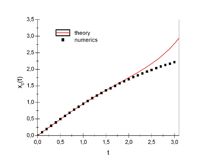
Fig. 4 depicts the trajectory of $x_{0}(t)$. The analytical curve which is given by the first three terms in formula (44) is a good approximation for a numerical trajectory if $t$ is not greater than $t\approx 2$. It gives the limitation for validity of the approximated partial solution $f_{-}(x,t)$.

The explicit formula for $x_{0}(t)$ enables us to obtain the function $G_{L}$ and the solution $f_{-}^{L}(x,t)$. Function $x_{0}(t)$, given by (44), is known up to $O(\sigma^{4})$ (including this term) so $t(w)$ can be obtained up to $O(\sigma^{0})$. The second formula in (43) gives

$$G_{L}(w)=-\frac{3}{8}\left(\frac{2}{\sigma^{2}}\right)^{1/3}w^{4/3}-\frac{4}{135}w^{2}+O(\sigma^{2/3}).$$ (45)

Finally, we obtain the partial solution $f_{-}^{L}(x,t)$ of the form

$$f_{-}^{L}(x,t)= - \frac{1}{540}(151x-119t)(x-t)-\frac{\sigma^{2}}{256}(x+t)^{2}+\frac{\sigma^{4}}{8640}(x+t)^{4}-$$ (46)

$$- \frac{3}{8}\left(\frac{2}{\sigma^{2}}\right)^{1/3}(x-t)^{4/3}.$$

Figure 5: Evolution of approximated analytical solution $f(x,t)$ for $\sigma^{2}=0.1$.

Figure 6: Numerical solution $f(x,t)$ for $\sigma^{2}=0.1$.

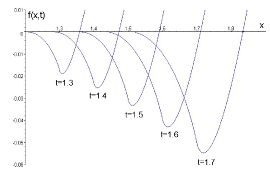
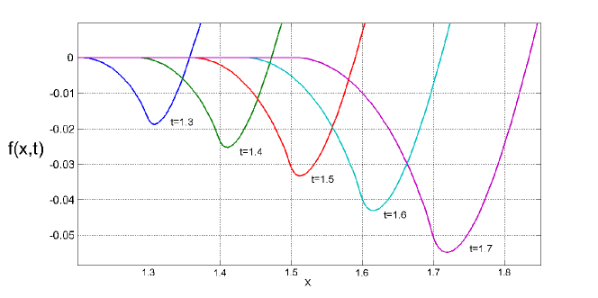
We note that the singular term $\sim\sigma^{-2/3}$ is present in the formulae (45) and (46). There is nothing unexpected in this fact because for small times the function $x_{0}(t)-t$ has similar behaviour to the function $x_{1}(t)-t$ from the previous paragraph. Some snapshots of the solution $f(x,t)$ for first stage of evolution are presented in Figs. 5 and 6. There is a very good agreement between numerical and analytical solutions untill $t\approx 2$.

3.5 Behaviour for later times $t>t^{*}$

In the current section we study a numerical solution for the s-K-G model with $\lambda=-0.1$. The solution at $t=0$ obeys following conditions

$$f(x,0)=\frac{1}{4}x^{2}\Theta(x),\qquad\partial_{t}f(x,t)|_{t=0}=0.$$

We focus on times $t>t^{*}$, where $t^{*}\approx 4.9673$. The trajectories of zeros of $f(x,t)$ up to $t=25$ are depicted in Fig. 7.

Figure 7: Trajectories of zeros.

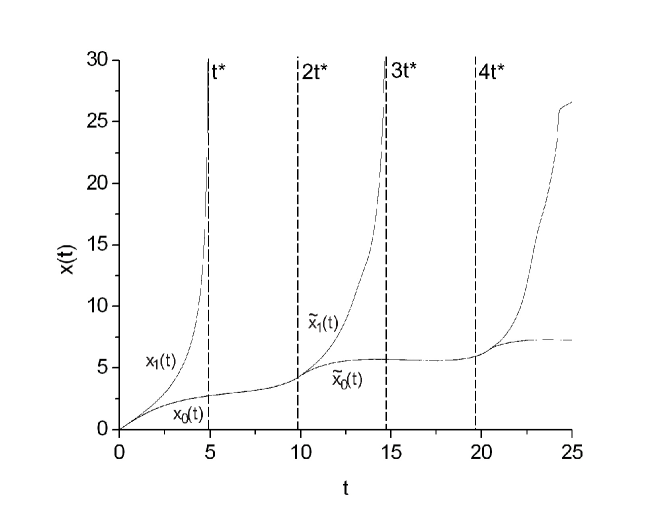
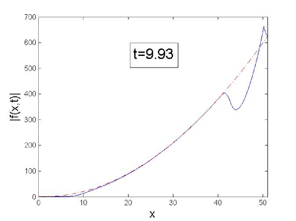
Zero $x_{0}(t)$ decelerates up to time $t\approx t^{*}$, then it accelerates up to $t\approx 2t^{*}$ when it reaches the velocity $v=1$. At this moment a very interesting phenomenon occurs. Zero $x_{0}(t)$ splits into a pair of zeros $\widetilde{x}_{0}(t)$ and $\widetilde{x}_{1}(t)$ that move similarly to $x_{0}(t)$ and $x_{1}(t)$. Numerical values of $\widetilde{x}_{1}(t)$ increase rapidly for $t\rightarrow 3t^{*}-$, which suggests that function $\widetilde{x}_{1}(t)$ has a vertical asymptote at $t=3t^{*}$. This phenomenon seems to have an almost periodic character.

One can show by an elementary calculation (we skip the proof) that the point $x_{0}$, at which the trivial solution ($f=0$) and a nonzero solution are matched so that the first right-hand spatial derivative of $f$ at $x_{0}$ is equal to zero, can not move with velocity $v\geq 1$. The solution $f(x,t)$, that consists of the partial solutions matched at the points that move with the velocity $v\neq 1$, has to be smooth (i.e first derivative is continuous) at the matching points. We can conclude that an accelerating zero, that is a matching point of the trivial partial solution $f=0$ and other nonzero partial solution, cannot move faster than $v=1$ without changing its character. This change means that the first spatial derivative of the field $f(x,t)$ is nonzero at this point. It is possible provided that an additional zero, that moves with velocity $v<1$, appears. The segment of $x$ axis between those two zeros widens. Such segment is a support of a partial solution of the second kind. At the moment when $x_{0}$ reaches the velocity $v=1$ the solution $f(x,t)$ returns with good approximation to its self-similar initial data (3.5) (see Fig. 8).

Figure 8: Absolute value of the solution $f(x,t)$ at $t=2t^{*}$ - the solid line, and the parabola of self-similar initial data - dashed line. A discrepancy at the right-hand side is a pure numerical effect caused by finite size of the grid.

4 Summary

A study of perturbed field-theoretic models with V-shaped potential and the scaling symmetry can give some knowledge that are properties of more general field models with potentials that are sharp at its minima. One of the simplest example of such models is the s-G model with perturbation that introduces an additional linear term to the field equation, which gives the s-K-G model. We have found that such a perturbation is responsible for some new effects. For the same initial data the differences between solutions in the s-G and the s-K-G models are caused by this linear term.

The first observation comes from analysis of trajectories of zeros. The zeros of the self-similar solutions in the s-G model move with constant velocities, whereas velocity of zeros of solutions in the s-K-G model is not monotonous. Moreover, their accelerations and decelerations also depend on time. Nevertheless, for small times $t\ll 1$ both the acceleration and the deceleration of zeros are proportional to the perturbation parameter $\lambda$. This fact can be useful as a phenomenological criterion that allows us to calculate the parameter $\lambda$ from experimental data.

We can also point out the second qualitative difference between these models. There are partial solutions in the s-K-G model that supports expand from zero to infinite size within a finite time. It is possible provided that the other partial solutions disappear simultaneously . For instance, the partial solution $\phi_{1}=\frac{1}{4}(x^{2}-t^{2})$ at $[t,\infty)$ in the s-G model disappears when $t\rightarrow\infty$, whereas the partial solution $f_{+}$ in the s-K-G model disappears when $t\rightarrow\frac{\pi}{2\sigma}$.

One of the most interesting results that have been obtained from approximated formulae for partial solutions $f_{-}^{R}(x,t)$ and $f_{-}^{L}(x,t)$ is an observation that these partial solutions contain singular terms proportional to $\lambda^{-1/3}$. It suggests that (apart from technical obstacles) the partial solution $f_{-}(x,t)$ can not be represented in the series form in the similar way to $f_{+}(x,t)$.

The last observation is mainly numerical. The trajectories of zeros of the solution $f(x,t)$ are almost periodic. We have proposed here a hypothesis that the period has the value $2t^{*}=\frac{\pi}{\sigma}$, where $t^{*}$ has been obtained from analytical calculations - it is the characteristic time for which the trajectory of zero $x_{1}(t)$ has a vertical asymptote. Our hypothesis agrees quite well with the numerical data. The periodicity for longer than investigated times is an open question. In our study the solutions $f(x,0)$ and $f(x,2t^{*})$ are very similar which means that the solution $f(x,t)$ returns to the self-similar initial data even though the scaling symmetry is broken.

An important and open question is the behaviour of solutions of the s-K-G model for other self-similar initial data or more general initial data. In the group of general initial data the most interesting are these for which an initial field configuration has a finite energy (the energy of the self-similar solutions has an infinite value). Finally, there are, of course, a variety of perturbations of the potential $V(\phi)=|\phi|$ that can be studied, nevertheless, it is clear that for most of them analytical results can be obtained only in approximation.

5 Acknowledgements

The author is grateful to Tomasz Tyranowski for his assistance in numerical work and valuable discussions as well as to Henryk Arodź, Andrzej Wereszczyński and Jakub Lis for discussions and remarks.

References

- [1] H. Arodź, P. Klimas and T. Tyranowski, Acta Phys. Pol. B36, 3861 (2005).
- [2] H. Arodź, P. Klimas and T. Tyranowski, Phys. Rev. E73, 046609 (2006).
- [3] P.Klimas Acta Phys. Pol. B38, 21 (2007).
- [4] H. Arodź Acta Phys. Pol, B33, 1241 (2002).
- [5] P. Rosenau, J. M. Hyman Phys. Rev. Lett., 70, 564 (1993).
- [6] F. Cooper, H. Shepard and P. Sodano Phys. Rev., E48, 4027 (1993).
- [7] P. Rosenau and A. Pikovsky Phys. Rev. Lett., 94, 174102 (2005).
- [8] C. Adam, J. Sánchez-Guillén and A. Wereszczyński hep-th/0705.3554
- [9] H. Arodź, P. Klimas and T. Tyranowski preprint hep-th/0710.2244
- [10] H. Arodź, P. Klimas and T. Tyranowski Acta Phys. Pol, B38, 3099 (2007).
- [11] C. Adam, N. Grandi, J. Sánchez-Guillén and A. Wereszczyński preprint hep-th/0711.3550