Autoregressive Time Series Forecasting of Computational Demand
Abstract
We study the predictive power of autoregressive moving average models when forecasting demand in two shared computational networks, PlanetLab and Tycoon. Demand in these networks is very volatile, and predictive techniques to plan usage in advance can improve the performance obtained drastically.
Our key finding is that a random walk predictor performs best for one-step-ahead forecasts, whereas ARIMA(1,1,0) and adaptive exponential smoothing models perform better for two and three-step-ahead forecasts. A Monte Carlo bootstrap test is proposed to evaluate the continuous prediction performance of different models with arbitrary confidence and statistical significance levels. Although the prediction results differ between the Tycoon and PlanetLab networks, we observe very similar overall statistical properties, such as volatility dynamics.
1 Introduction
Shared computational resources are gaining popularity as a result of innovations in network connectivity, distributed security, virtualization and standard communication protocols. The vision is to use computational power in the same way as electrical power in the future, i.e. as a utility. The main obstacle for delivering on that vision is reliable and predictable performance. Demand can be very bursty and random, which makes it hard to plan usage to optimize future performance. Forecasting methods for aiding usage planning are therefore of paramount importance for offering reliable service in these networks.
In this paper we study the demand dynamics of two time series from computational markets, PlanetLab111http://www.planet-lab.org and Tycoon222http://tycoon.hpl.hp.com. Our main objective is to study the prediction abilities and limitations of time series regression techniques when forecasting averages over different time periods. Here we focus on hourly forecasts that could be applied for scheduling jobs with run times in the order of a few hours, which is a very common scenario in these systems. The main motivation for this study was that an exponential smoothing technique used in previous work [12], was found to perform unreliably in a live deployment.
The general evaluation approach is to model the structure of a small sample of the available time series, and assume the structure is fixed over the sample set. Then perform predictions with regularly updated model parameters and benchmark those predictions against a simple strategy using the current value as the one-step-ahead forecast (assuming a random walk).
We focus our study on the following questions.
-
•
Can a regression model perform better than a strategy assuming a random walk with no correlations in the distant past?
-
•
How much data into the past are needed to perform optimal forecasts?
-
•
How often do we need to update the model parameters?
The answers to these questions depend on both the size of the sliding window used for the forecast and on the length of the forecast horizon. Our goal is to give general guidelines as to how forecasts should be performed in this environment.
When predicting demand in computational networks instantaneous, adaptive, flexible, and light-weight predictors are required to accurately estimate the risk of service degradation and to quickly take preemptive actions. With the increased popularity of virtualized computational markets such as Tycoon, this need for prediction takes a new dimension. Successful forecasts can now reduce the cost of computations more directly and explicitly. However, high volatility and non-stationarity of demand complicates model building and reduces prediction reliability.
The main objective of this study is to investigate which time series models can be used when predicting demand in computational markets, and how they compare in terms of predictive accuracy to simpler random walk and exponential smoothing models. Since modeling and parameter estimations need to adapt quickly to regime shifts, a simple fixed static model of the entire series is not likely to produce any good results. In this work we make a compromise and fix the structure of the model but update the parameter estimates continuously.
The contribution of this work is threefold:
-
•
we perform ARIMA modeling and prediction of Tycoon and PlanetLab demand,
about predictor model performance,
-
•
and we identify common statistical properties of PlanetLab and Tycoon demand.
The paper is structured as follows. In Section 2 our evaluation approach is discussed, and in Section 3 we model and predict the PlanetLab series. In Section 4 we perform the same analysis for the Tycoon series. Then we compare the analyses in Section 5 and discuss related work in Section 6 before concluding in Section 7.
2 Evaluation Method
In this section, we describe the method used to construct models and to evaluate the forecasting performance of models of the time series studied.
2.1 Modeling
We first construct an autoregressive integrated moving average (ARIMA) model of a small sample of the time series in order to determine the general regression structure of the data. The rationale behind this approach is that the majority of the data should be used to evaluate the forecasting performance. During forecasting the model parameters are refit, and to compensate for possible changes in structure we evaluate a number of similar benchmark models. Furthermore, in a real deployment, we ideally want to re-evaluate the regression structure infrequently compared to the number of times the structure can be used for predictions to make it viable. The sample used for determining the regression structure is discarded in the forecasting evaluation to keep the predictions unbiased. Conversely, no measured properties of the time series outside of the sample window are used when building the models of the predictors.
The general model and the benchmark models are then fit to partitions of the data in subsequent time windows. In each time window the model parameters are re-evaluated. The fitted model then produces one, two, and three-step-ahead forecasts. The forecasts are thus conditioned on the assumption of a specific structure of the model. The size of the time windows are made small enough to allow a large number of partitions and thus also independent predictions, and kept big enough for the ARIMA maximum likelihood fits to converge.
2.2 Forecast
The fitted ARIMA model structure is compared to two standard specialized ARIMA processes. The first benchmark model used is the random walk model (RW), ARIMA(0,1,0), which always produces the last observed value as the forecast. The second model is the Exponentially Weighted Moving Average (EWMA), a.k.a. the exponential smoothing model, which can be represented as an ARIMA(0,1,1) or IMA(1,1) process producing forecasts with an exponential decay of contributions from values in the past. This representation is due to Box et al. [2] who showed that the optimal one-step-ahead forecast of the IMA(1,1) model with parameter is the same as the exponential smoothing value with factor .
For each set of time-window predictions performed, the mean square error (MSE) is computed. To facilitate comparison, the MSEs are normalized against the random walk model as follows
| (1) |
where is the MSE of the model studied, and is the MSE of the benchmark. Thus an means that the model generated more accurate forecasts than the benchmark. Hence, we have
| (2) |
where is the probability density function (PDF) of . Thus we have constructed a statistic for evaluating the models based on the cumulative distribution function (CDF) of the log ratio of the model and the RW benchmark MSEs, which we call normalized distribution error or NDE. This statistic is similar in spirit to the MSE measurement itself, but to avoid a bias towards symmetric error distributions, we base our statistic on the median as opposed to the mean. One might argue that highly incorrect predictions, therefore, are not penalized strongly enough, but we are more interested in the reliability aspect of predictions here, i.e., which model can be trusted to perform better in most cases. If the error distribution has many outliers it should be reflected in the width of the confidence bound instead. We thus focus next on building such unbiased confidence bounds.
2.3 Statistical Test
With the NDE statistic we have a metric to decide when a model performs better than a benchmark, but in order to render claims of statistical significance and prediction confidence bounds, a measure of error variance is needed. Due to a limited set of original data points (one MSE for each sample window size), the approach is to use bootstrap sampling based on the empirical distribution of . Using (2) the null hypothesis is , that is, the studied model predicts more accurately than the benchmark in a majority of the cases. The alternative hypothesis is then obviously that the studied model performs worse than the benchmark in a majority of the cases. The bootstrap algorithm is as follows
-
1.
Calculate the values for the different sample windows
-
2.
Pick samples of size from the values with replacement
-
3.
Calculate the and the per cent points from the empirical distribution function of the selected samples, as the lower and upper confidence bounds respectively
-
4.
Reject the null hypothesis and accept the alternative hypothesis if the upper bound is , and accept the null hypothesis and reject the alternative hypothesis if the lower bound is at the 100 per cent significance level. If the bound overlaps with we say that the model performs on par with the benchmark.
R code which implements this test is available in Appendix A. This Monte Carlo bootstrap algorithm is used for two reasons, first to avoid making any assumptions about the distribution of the normalized MSEs in the test, and second to easily map MSE uncertainty to bounds on our NDE statistic. The NDE bound can be interpreted as there being a 100 per cent likelihood of the model performing better than the random walk model in 100 per cent to 100 per cent of the cases.
In the following sections we apply this evaluation method to the PlanetLab and Tycoon series.
3 PlanetLab Analysis
PlanetLab (PL) is a planetary-scale, distributed computing platform comprising approximately 726 machines at 354 sites in 25 countries, all running the same Linux based operating system and PlanetLab software. The user community is predominantly computer science researchers performing large-scale networking algorithm and system experiments. The time series is from December 2005 to December 2006. We calculate demand by aggregating the load value across all hosts and averaging in hourly intervals with a 5-min sample granularity. This load measures the number of processes that are ready to run on machine.
3.1 Model
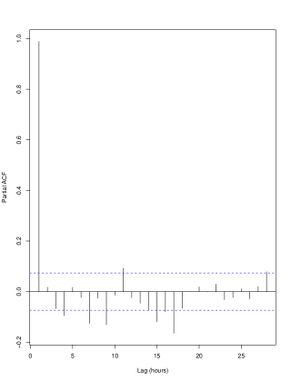
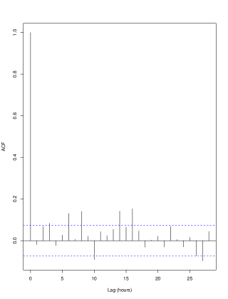
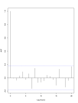
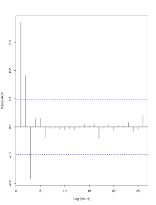
We select the first month of the trace (707 values out of 8485) as our sample to construct the general ARIMA model. The sample series is shown in Figure 1. There is one big spike in the sample, and we might be tempted to treat it as an outlier, but as seen from the full trace these spikes are quite common and thus need to be accounted for in our model. We instead perform a Box-Cox [1] transform to address non-stationarity in variance. The Box-Cox plot for the sample is shown in Figure 1(c). A value of is thus used to transform the series prior to the ARIMA analysis. This value is somewhere between a and a (no) transform. From Figure 2 we note that the ACF has a slow decline in correlation, and that the PACF is near unit root in lag 1. Now to formally test for unit root we perform the augmented Dickey-Fuller test [5], and obtain a t-statistic of which has an absolute value less than the per cent critical value , so we cannot reject the null hypothesis of a unit root.
Therefore, we difference the series and then see that the differenced ACF in Figure 2(c), does not exhibit any clearly significant correlations. Hence, we model the series as as an ARIMA(0,1,0) process or random walk. We note that there appears to be small significant seasonal correlations around lags 6,8,10,14 and 16. But we decide to ignore those because of our small sample size, and to keep the predictor simple. To summarize, the entertained model is
| (3) |
where is the backshift operator and is the residual white noise process. A Box-Ljung test [8] of serial correlations of the residuals of this model gives a value of and a p-value of for degrees of freedom, so there is still structure unaccounted for. Our tests showed that at least an ARIMA(16,1,0) model was needed before the Box-Ljung test succeeded, which is not practical for our purposes, so we stick to our ARIMA(0,1,0) model. Because this model is one of our standard benchmarks (RW) we also add an ARIMA(1,1,0) model to our evaluation to simplify comparison.
3.2 Forecast
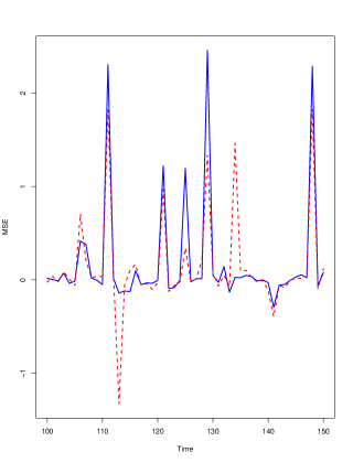
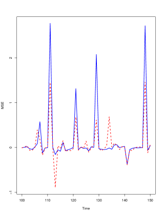
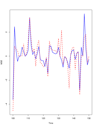
We now compare the MSE of the one-, two- and three-step-ahead forecasts of the RW, EWMA, and ARIMA(1,1,0) models. The time windows used for predictions range from to hours. Each empirical normalized MSE distribution thus has measurements. The evaluation of the forecasts of the ARIMA(1,1,0), and the exponential smoothing models against the random walk model can be seen in Figure 3. We note that a value less than in the plot means that the model predictor performed better than the random walk predictor. We observe that both the ARIMA(1,1,0) and the exponential smoothing model predictors seem to perform better than the random walk predictor for the two and three-step ahead predictions. We further note that there are more high peaks than deep valleys both for ARIMA(1,1,0) and EWMA, and that the EWMA peaks are lower. This pattern indicates that the RW model is more immune to extreme level shifts, and that EWMA handles these shifts better than ARIMA(1,1,0).
Next, we use the statistical test constructed in the previous section to verify the significance of the differences.
3.3 Statistical Test
Table 1 shows the NDE bound results for the PlanetLab models at significance level 5% where was set to . The random walk row displays the errors in proportion to the true value observed, calculated as
| (4) |
where is the predicted value at time and is the actual value; and is the number of time windows used in the test (). We see that the errors ranged from % to % with the longer horizon forecasts performing worse. From the NDE statistic bounds for the ARIMA(1,1,0) and EWMA rows in Table 1 we can conclude that the ARIMA(1,1,0) model generates predictions on par with the random walk model, for one and two-step-ahead predictions, and better at significance level per cent for three-step-ahead forecasts. The EWMA model performs better for longer forecasts but not at a significant enough level to pass our test. To summarize, the only strong conclusion we can draw from these simulations is that the ARIMA(1,1,0) predictor performed better than a random walk predictor for three-hour ahead forecasts, but in general the RW model selected performs relatively well.
| 1 SE | 2 SE | 3 SE | |
|---|---|---|---|
| RW | |||
| ARIMA(1,1,0) | |||
| EWMA |


4 Tycoon Analysis
Tycoon is a computational market where resources, such as CPU, disk, memory, and bandwidth can be purchased on demand to construct ad-hoc virtual machines. The price of the resources is in direct proportion to the demand, in that the cost of a resource share is dynamically calculated as the ratio between the bid a user places on the resource and the bids all other users of that resource place. The Tycoon network currently comprises about 70 hosts. Usage is sparse and spiky, and is mostly generated from different test suites that are designed to evaluate the system. A trace was recorded of the aggregated CPU price in hourly intervals with a 10-min granularity during a period of 17 days in July-August 2007.
4.1 Model
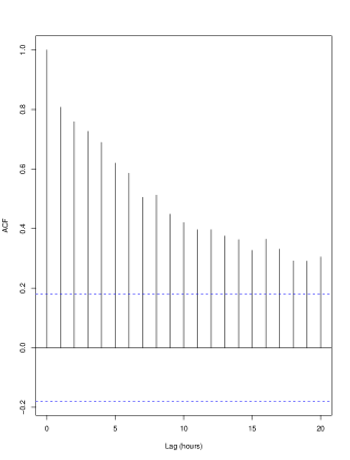
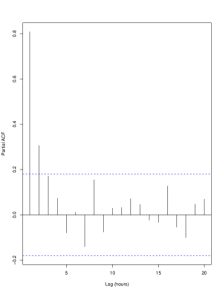
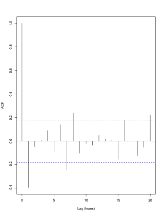
We select the first five days of the trace (119 values out of 404) as our sample to construct the general ARIMA model. The sample and the full series are shown in Figure 4. Due to suspected non-stationarity in variance a Box-Cox transform is again performed. As seen in Figure 4(c), the value obtained was . We note that the ACF decays slowly and the PACF has a high first lag in Figure 5. So we again difference the series. Now the ACF shows only one significant lag, so we can model it as an IMA(1,1) process. The correlations of the residuals of this model can be seen in Figure 5(d). To summarize, the entertained model is
| (5) |
where is the backshift operator and is the residual white noise process. The coefficient was found to be statistically significant at a per cent significance level, and was fit to . A Box-Ljung test of serial correlations of the residuals of this model gives a value of and a p-value of for degrees of freedom, hence we conclude that the model does not have any serial correlations and is accurate. Because this model is one of our standard benchmarks (EWMA) we also add an ARIMA(1,1,0) model to our evaluation to simplify comparison.
4.2 Forecast
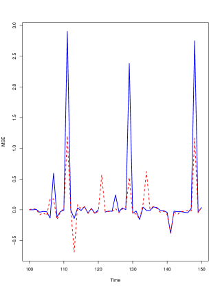
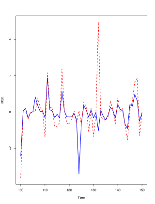
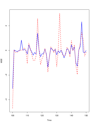
We now compare the MSE of the forecasts of the RW, EWMA, and ARIMA(1,1,0) models. The model parameters are evaluated before each forecast. The time-window used for model fitting ranged from 50 hours to 100 hours into the past, and thus again measurements were generated. The evaluation of the ARIMA(1,1,0), and the exponential smoothing models against the random walk model is shown in Figure 6. We recall that a value less than in the plot means that the model predictor performed better than the random walk predictor. It is not as clear as in the PlanetLab series that RW has fewer extremes of bad predictions. However the ARIMA(1,1,0) model does seem to produce less extreme peaks and valleys than EWMA, i.e. the opposite of what was observed for the PlanetLab data. Due to high volatility it is difficult to draw any conclusions about which model performs best from these plots, so we again have to resort to our statistical test.
4.3 Statistical Test
Table 2 shows the NDE bound results for the Tycoon models at significance level 5 per cent where was set to . We see that the RW model performed much worse for this time series compared to in the PlanetLab series. Average errors range from per cent to per cent. This apparent difficulty in predicting the series also reflects the results. We see that both the ARIMA(1,1,0) and EWMA models performed on par with RW for all forecasts. So at the per cent significance level no strong conclusions can be drawn about which model performed best. We however note, for the three step-ahead forecasts, that ARIMA(1,1,0) is close to being significantly better than RW, and for one step-ahead forecast, EWMA is close to being significantly worse than RW. The same pattern is apparent here, as in the PlanetLab data; the higher order ARIMA models perform better for longer forecasts.
| 1 SE | 2 SE | 3 SE | |
|---|---|---|---|
| RW | |||
| ARIMA(1,1,0) | |||
| EWMA |


5 Series Comparison
In this section we compare the dynamics of the PlanetLab series to the Tycoon series using the full traces, and give both quantitative and qualitative explanations to the differences.
Table 3 shows the range and the quartiles of the series, normalized by the series mean. The Tycoon series has a median which is further away from the mean, and the range of values is slightly tighter. The narrower range is expected because of the time horizon difference in the two series. However, overall the statistics for PlanetLab and Tycoon are strikingly similar. This is a bit surprising since Tycoon is just in an early test phase with very limited usage and demand, whereas PlanetLab is a mature system that has been in operation for several years.
| Min | Q1 | Median | Q3 | Max | |
|---|---|---|---|---|---|
| PlanetLab | .494 | .811 | .936 | 1.12 | 6.55 |
| Tycoon | .452 | .763 | .860 | 1.10 | 5.70 |
The volatility statistics of the two series are compared in Table 4. We conclude that the variance is higher in Tycoon, but the right tail of the PlanetLab series distribution is longer, and the PlanetLab series is also more prone to outliers. Again it is remarkable how closely the tail and outlier behavior of the much smaller Tycoon sample follows the PlanetLab statistics.
| Coef of Variation | Skewness | Kurtosis | |
|---|---|---|---|
| PlanetLab | .362 | 4.03 | 28.29 |
| Tycoon | .511 | 3.67 | 24.38 |
To determine whether any of these series exhibit heteroskedasticity, we take the squared residuals from an ARIMA model of the full series and fit an AR model. Then according to Engle [7] heteroskedasticity exists if
| (6) |
where is the number of values in the series, the order of the AR model fit to the squared residuals, is the density function with degrees of freedom, and is the significance level. The complete PlanetLab series follows an ARIMA(3,1,0) model and the complete Tycoon series follows an IMA(1,2) model. The residuals and their squares of these models can be seen in Figure 7.
We find that both the PlanetLab and Tycoon series pass the significance test at the per cent significance level. Furthermore, both the Tycoon and the PlanetLab squared residuals follow AR(3) models, i.e., they have very similar volatility dynamics structure.
It is easy to see that this heteroskedasticity could cause more outliers and higher kurtosis in a static model. Intuitively, if the first moment fluctuates, the second moment increases, and similarly if the second moment fluctuates there is a greater likelihood of more spikes or AR model outliers, which would increase the kurtosis. High volatility and dynamics in structure could also explain why ARIMA predictions assuming static volatility and regression structure perform so poorly compared to a simple random walk predictor. However, we note that a random walk predictor does not accurately estimate risk of high demand, which is more apparent for forecasts with a longer future time horizon. An alternative approach to studying volatility and risk over time is the approach of measuring long term memory or dependence. This was done in [11], and we found that non-Gaussian long term dependencies did exist, which could cause so called workload flurries with abnormally high demand.
The ARIMA(1,1,0) model performs better in PlanetLab than in Tycoon, which may indicate that PlanetLab has longer memory of past values than Tycoon. This may be attributed to the shorter sample period and the nature of the applications currently running on Tycoon; mostly short intense test applications.


6 Related Work
The algorithm used for the statistical test of significant differences in predictor performance was inspired by the Monte Carlo bootstrap method introduced by Efron in [6] and popularized by Diaconis and Efron in [4]. The bootstrap method is typically used as a non-parametric approach to making confidence claims. We, use it to expand a short sample into a bigger one without any distributional assumptions about the MSE terms. A more typical usage is to shrink a large sample into multiple smaller random samples that are easier to make statistical claims about collectively.
Tycoon usage has not been statistically investigated before. Previous work on the computational market characteristics of Tycoon has used PlanetLab and other super computing center job traces as a proxy for expected market demand [12] or made simple Gaussian distribition, and Poisson arrival process assumptions [11].
In this work we support the study of PlanetLab as a proxy for Tycoon demand, by verifying a large number of statistical commonalities, both in terms of structure of series and in terms of optimal predictor strategies. Chun and Vahdat [3] have analyzed PlanetLab usage data but not from a predictability viewpoint. Their results include observations of highly bursty and order of magnitude differences in utilization over time, which we also provide evidence for. We note that the PlanetLab trace that Chun and Vahdat studied was from 2003.
Oppenheimer et al. [10] also analyze PlanetLab resource usage and further evaluate usage predictors and conclude that mean reverting processes such as exponential smoothing, median, adaptive median, sliding window average, adaptive average and running average all perform worse than simple random walk predictors and, what they call, tendency predictors which assume that the trend in the recent past continues into the near future. They further notice no seasonal correlations over time due to PlanetLab’s global deployment. We do see some seasonal correlations in our initial time series analysis but not significant enough to take advantage of in predictions. Further, our evaluation approach follows the traditional ARIMA model evaluation method, and we provide a statistical test to verify and compare prediction efficiency. One major difference between our studies and thus also the conclusions is that Oppenheimer et al. only considered one-step ahead predictions whereas we also consider two, and three-step ahead predictors to do justice to the models considering correlations beyond the last observed step. We finally note that they studied PlanetLab data from August 2004 to January 2005, whereas we studied more recent data from December 2005 to December 2006.
7 Conclusions
This work set out to study the predictive power of regression models in shared computational networks such as PlanetLab and Tycoon. The main result is that no significant evidence was found that higher order regression models performed better than random walk predictions. The exception was for three-step ahead predictions in PlanetLab where an ARIMA(1,1,0) model outperformed the random walk model.
The study also shows the difficulty in composing a model from a sample and then using this model in predictions if the structure of the series is changing over time as in the Tycoon case.
Our study highlighted a number of statistical similarities between Tycoon and PlanetLab, such as volatility structure, outlier likelihood, and heavy right tails of density functions, which motivates further studies and comparisons of workloads to improve forecasting.
The ARIMA models were refitted for every 50 to 150 hours to provide as accurate models of the recent past as possible, but the overall structure of the model was fixed as the one obtained from the fit of the sample series. Larger fitting windows were tested for the PlanetLab data without any effect in the results, but larger windows could not be tested for the Tycoon series due to the limited trace time frame (17 days). There was however a clear pattern that the higher order ARIMA models performed better in the two and three-step ahead forecasts compared to the random walk model.
To summarize, we have exemplified the difficulties in modeling significant regressional parameters for computational demand dynamics, even if the model is very generic and the model parameters are re-estimated frequently. It was found difficult to improve on the random walk process model for one-step-ahead forecasts, which is a bit surprising (and contradictory to the main hypothesis in [9]) given that RW processes, in theory, should generate a normal distribution of demand whereas the actual measured demand distribution was very right skewed and heavy tailed, both in the PlanetLab and the Tycoon series.
We do however see that higher order regressional parameters can improve the two-step and three-step ahead forecasts. More work is needed to determine how these models should be discovered and dynamically updated. One possible extension is to see if there is an improvement in predictor performance if the model is allowed to changed dynamically as well as the parameters based on observed ACF and PACF behavior. More work is also needed to determine the computational overhead of the more complicated regressional models and the calculations of fits and predictions. Accurate random walk predictors can be built very easily with virtually no overhead, so the improvement in accuracy needs to be significant to be worthwhile. This work does however show that there is a potential for improvement of longer forecasts.
Acknowledgments
I would like to thank Professor Magnus Boman for his detailed comments on earlier versions of this paper; and Professor Raja Velu and Kevin Lai for providing the inspirational ideas underlying this study.
References
- [1] G. Box and D. R. Cox. An analysis of transformations. Journal of the Royal Statistical Society, B(26):211–252, 1964.
- [2] G. Box, G. M. Jenkins, and G. Reinsel. Time Series Analysis, Forecasting and Control (3rd ed.). Prentice-Hall, Englewood Cliffs, NJ, 1994.
- [3] B. N. Chun and A. Vahdat. Workload and failure characterization on a large-scale federated testbed. Technical report, Intel Research Berkley Technical Report IRB-TR-03-040, 2003.
- [4] P. Diaconis and B. Efron. Computer-intensive methods in statistics. Scientific American, (6):116–130, 1983.
- [5] D. A. Dickey and W. A. Fuller. Likelihood ratio statistics for autoregressive time series with a unit root. Econometrica, (49):1057–1072, 1981.
- [6] B. Efron. Bootstrap methods: Another look at the jackknife. The Annals of Statistics, 7(1):1–26, 1979.
- [7] R. Engle. Autoregressive conditional heteroscedasticity with estimates of the variance of united kingdom inflation. Econometrica, 50:987–1007, 1982.
- [8] G. M. Ljung and G. E. P. Box. On a measure of lack of fit in time series models. Biometrica, (65):553–564, 1978.
- [9] B. Mandelbrot and R. L. Hudson. The (Mis)behavior of Markets: A Fractal View of Risk, Ruin, and Reward. Basic Books, New York, NY, USA, 2004.
- [10] D. Oppenheimer, B. Chun, D. Patterson, A. C. Snoeren, and A. Vahdat. Service placements in a shared wide-area platform. In USENIX’06: Annual Technical USENIX Conference, 2006.
- [11] T. Sandholm and K. Lai. Prediction-based enforcement of performance contracts. In GECON ’07: Proceedings of the 4th International Workshop on Grid Economics and Business Models, 2007.
- [12] T. Sandholm and K. Lai. A statistical approach to risk mitigation in computational markets. In HPDC ’07: Proceedings of the 16th ACM International Symposium on High Performance Distributed Computing, 2007.
Appendix A Bootstrap Test R-Code
-
predict_arima <- function(x,ord, window, horizon, mse, lambda) { n = (length(x)-window-2)/window errors=c() for (i in 0:n) { start_index = i * window stop_index = start_index + window -1 outcome_index = start_index + window model = arima(boxcox_transform(x[start_index:stop_index],lambda), \ order=ord,method="ML") pred = predict(model, n.ahead=horizon) if (mse) { errors = c(errors, (x[outcome_index+horizon-1] - \ boxcox_inverse(pred$pred[horizon],lambda))^2) } else { errors = c(errors, abs((x[outcome_index+horizon-1] - \ boxcox_inverse(pred$pred[horizon],lambda))/x[outcome_index+horizon-1])) } } mean(errors) } evaluate_arima <- function(x,ord,from,stop,step,walk,horizon,mse,lambda) { arima_mse = c() walk_ind = 1 to = round((stop - from)/step) + from for (i in from:to) { window = from + ((i-from)*step) pred = predict_arima(x,ord,window,horizon,mse,lambda) if (length(walk) > 0) { pred = pred / walk[walk_ind] walk_ind = walk_ind + 1 } arima_mse=c(arima_mse,pred) } arima_mse } bootstrap_test <- function(x,sample_size,alpha) { n=length(x) x_sample = c() for (i in 1:sample_size) { x_sample=c(x_sample,ecdf(sample(x,n,replace=T))(0)) } sort_sample = sort(x_sample) c( sort_sample[round(sample_size*alpha/2)], \ sort_sample[round(sample_size*(1-alpha/2))] ) } evaluate_walk_exp <- function(x,ord,horizons,from,to,step,alpha,samples,lambda) { exp_errors = c() arima_errors = c() walk_errors = c() x_evals = c() x_exps = c() for (i in 1:horizons) { walk_error = evaluate_arima(x,c(0,1,0),from,to,step,c(),i,mse=F,lambda) walk_errors = c(walk_errors, mean(walk_error), mean(walk_error)) x_walk = evaluate_arima(x,c(0,1,0),from,to,step,c(),i,mse=T,lambda) x_eval = evaluate_arima(x,ord,from,to,step,x_walk,i,mse=T,lambda) x_exp = evaluate_arima(x,c(0,1,1),from,to,step,x_walk,i,mse=T,lambda) x_evals = cbind(x_evals, x_eval) x_exps = cbind(x_exps, x_exp) # Pr(EXP < RW) exp_errors = c(exp_errors,bootstrap_test(log(x_exp),samples,alpha)) # Pr(ARIMA < RW) arima_errors = c(arima_errors,bootstrap_test(log(x_eval),samples,alpha)) } errors = cbind(walk_errors,arima_errors,exp_errors) attr(errors,’arima’) = x_evals attr(errors,’exp’) = x_exps errors }