Fractal dimension of domain walls in the Edwards-Anderson spin glass model
Abstract
We study directly the length of the domain walls (DW) obtained by comparing the ground states of the Edwards-Anderson spin glass model subject to periodic and antiperiodic boundary conditions. For the bimodal and Gaussian bond distributions, we have isolated the DW and have calculated directly its fractal dimension . Our results show that, even though in three dimensions is the same for both distributions of bonds, this is clearly not the case for two-dimensional (2D) systems. In addition, contrary to what happens in the case of the 2D Edwards-Anderson spin glass with Gaussian distribution of bonds, we find no evidence that the DW for the bimodal distribution of bonds can be described as a Schramm-Loewner evolution processes.
pacs:
75.10.Nr, 75.40.MgWhereas the properties of long range Ising spin glasses are now well understood, after more than 20 years of work, the same cannot be said about short range spin glasses. This is true even for very simple models: the nature of the ordering of the low temperature phase of the two-dimensional (2D) Edwards-Anderson (EA) spin glass model EA is still being debated. Even though the fact that at EA models with Gaussian (EAG) and bimodal (EAB) bond distributions belong to two different universality classes seems well established, Amoruso2003 new studies Hartmann2007 of low energy excitations (fractal droplets) show that there is still room for discussion.
It has recently been suggested Amoruso2006 ; Bernard2007 that domain walls (DWs) can be described as Schramm-Loewner evolution (SLE) processes. These processes are Brownian walks of diffusion constant and fractal dimension . Furthermore, using conformal field theory the stiffness exponent (which characterizes the scaling of the DW energy) can be related to the fractal dimension via
| (1) |
This seems to be true for the 2D EAG, as for Hartmann2002 Eq. (1) gives , which is compatible with the best numerical estimate . Melchert2007 It is not clear, however, whether such a relation should hold for the 2D EAB, because of the high degeneracy of its ground state (GS). If it did, using the fact that the stiffness exponent seems to vanish, Hartmann5 Eq. (1) would yield .
In the EAB model the degeneracy of the GS precludes a clear-cut definition of the fractal dimension of the DW. For this reason, most of the estimates of are based on a scaling argument of Fisher and Huse, Fisher1 which states that the entropy of droplets of size should scale as . It must be stressed that this was originally proposed for systems with only one GS. The estimates obtained using this scaling range from to . Saul1993 ; Aromsawa2007 Even though very recently more direct measurements have been attempted, Roma2007 ; Weigel2007 in those works the sampling of the DWs was not controlled. Melchert2007 In Ref. Melchert2007, this problem is avoided and bounds are provided for the true : .
In this paper we present the results of an extensive numerical study of the fractal dimension of DWs, using a direct measure of their length. We have studied both 2D and 3D systems with Gaussian and bimodal distributions of bonds, but we have concentrated on the EAB model. For small systems we have calculated the exact average DW length. For larger systems an estimate of this quantity has been calculated by choosing only one pair of GSs. Even though the sampling we use is clearly not uniform, the values we obtain with this estimate coincide with the exact ones, for small systems. Our results show that, whereas in 3D is the same for EAB and EAG, in the 2D case the corresponding values are clearly different and, in particular, for the EAB, different from the value that would be obtained from Eq. (1) (assuming that ). In addition, we have performed one test to see whether DWs in 2D can be described as SLE processes. Even though for the EAG the result of this test is positive, for the EAB the outcome of the test is clearly negative.
We start by considering the Hamiltonian of the EA model for spin glasses EA on square and cubic lattices, , where is the spin variable and indicates a sum over nearest neighbors. The coupling constants are independent random variables chosen either from a bimodal () or Gaussian bond distributions, both with zero mean and variance one.
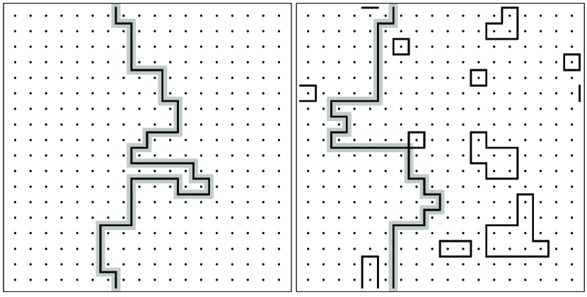
In 3D we have used periodic boundary conditions (BCs) in all directions, and in 2D we have studied two cases: periodic-periodic BCs and periodic-free BCs.
For the EAG the definition of the DW is straightforward: given a system we ‘perturb’ it by changing the sign of all the bonds in a column in 2D or plane in 3D (i.e. we introduce antiperiodic BCs in one direction) and compare the GS of the new system with that of the unperturbed one. The DW is simply the set of bonds which have ‘changed state’, i.e. those for which has changed its sign. It can be shown that in the dual lattice, the dual of the bonds that have changed can only form a path in 2D (or surface in 3D) notadual of length (or area) , that goes from one border of the lattice to the opposite one (see Fig. 1). is obtained from the relation , where is the sample average () of .
| EAB | EAG | |||||
|---|---|---|---|---|---|---|
| EAB | EAG | |||||
|---|---|---|---|---|---|---|
For the EAB one has to be a bit more careful because the GS is degenerated. If one performs the same procedure as above, but now with a random pair of GSs, one sees that many sets of bonds have changed state (see Fig. 1). Only one of these sets forms a structure that crosses the sample, as in the EAG. The other sets form loops of zero energy: they enclose clusters of spins that can be flipped without changing the energy of the sample. As these clusters are present both in the perturbed and the unperturbed systems, it is reasonable to define the DW of a given pair of GS, as only the structure that crosses the sample. In this case the characteristic length of the DW of a sample, , is defined as the average over all pair of GSs of the length of DWs, as defined above. In practice, to extract the DW in the EAB one has to look for the percolating structure in the dual lattice, both for 2D and 3D. For this we have used the algorithm of Hoshen-Kopelman. Hoshen1976 We have been careful to eliminate the loops (or closed surfaces) that stick to the DW (see Fig. 1 for an example).
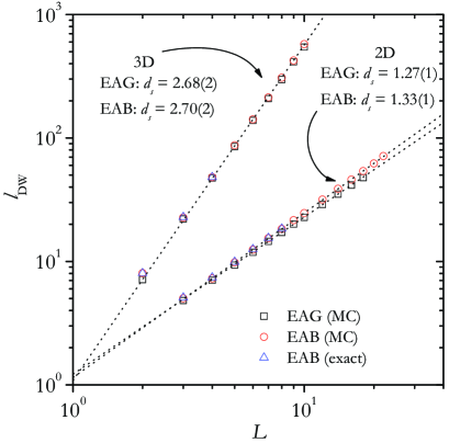
For small EAB samples we have obtained the exact value of the DW length by averaging over all pairs of GSs for each sample. To obtain all the GSs for systems with fully periodic BCs we have used a branch-and-bound algorithm. Hartwig1984 We have studied sizes up to in 2D and in 3D ( samples for each size). Results are shown in Fig. 2. This approach is not practical for larger sizes because of the fact that the number of GSs grows exponentially with . Landry Therefore, to estimate the average DW length for larger samples, we have resorted to a Monte Carlo (MC) algorithm to obtain one pair of random GSs for each sample (see Fig. 2).
The MC algorithm we have used is a variant of parallel tempering Hukushima1996 but suitably modified to find a ground state as quickly as possible. As in Ref. Hukushima1996, , we use a compound system or ensemble, that consists of noninteracting replicas of the system, each one associated to a different temperature in the interval , where the distance between consecutive temperatures is a constant. In general the heart of a parallel tempering algorithm consists of two routines that are performed alternately. One of them consists of a standard MC algorithm applied to each replica: in each elementary step, the update of a random selected spin of the ensemble is attempted with probability given by the Metropolis rule Metropolis . In the other routine, an exchange of two configurations between two replicas at consecutive temperatures is attempted with the probability defined in Ref. Hukushima1996, . In general, the unit time or MC step (MCS) of a parallel tempering algorithm consists of a fixed number of elementary steps of standard MC, followed by another fixed number of trials of replica exchange. To equilibrate the system a MCS defined as elementary steps of standard MC and only one replica exchange, is usually chosen. As we are only interested in reaching quickly a configuration of GS, we have used a different MCS: it consists of cycles, where a cycle is defined as only one elementary step of standard MC plus one replica exchange. After MCS, the algorithm stops and the configuration with minimum energy (among all configurations visited in all replicas in the simulation process) is stored. We have found that this algorithm is very efficient for reaching the GS: we have checked that, for the sizes studied with the parameters indicated in Tables I and II, our heuristic outputs a true GS with a probability larger than . In particular for 2D systems, we have verified this by calculating the ground states energies with an exact branch-and-cut algorithm DeSimone ; server and comparing them with the energies of the configurations we obtained (a detailed analysis of this algorithm will be published elsewhere Roma2008 ).
In our simulations, for each lattice size of EAB and EAG in both 2D and 3D systems we have used replicas with temperatures between to . The number of MCS and the number of samples analyzed for each sample size, is given in Tables I and II.
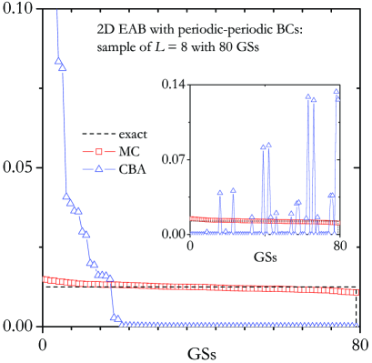
Interestingly, considering only one pair of GSs for each EAB sample leads to an estimate of the average DW length that is within only of its exact value (for small systems). This is good evidence that the MC algorithm is sampling the GS space almost uniformly. As our algorithm does not reach equilibrium we have checked explicitly that the sampling is indeed almost uniform. In Fig. 3 we show the distribution of GSs reached by our algorithm for a typical 2D sample with 80 GSs. It is instructive to compare our method with the sampling that results from the algorithm (hereafter called CBA) used by Cieplak and Banavar. Cieplak In this technique an infinitesimal noise is added to the couplings, and the GS of the system is obtained. Then, the same realization of the noise is added to the system with antiperiodic BCs and a new GS is obtained. The noise in the couplings breaks the degeneracy, and the fact that the same realization of the noise is used ensures that the resulting DW has no loops. Up to we have also used the CBA to analyze the same samples as with the branch-and-bound algorithm. As Fig. 3 shows, the sampling given by this technique is far from uniform. In fact, there is a large fraction of GSs that are not reached by it. In spite of this, the estimate of the average DW length given by the CBA is within of its exact value (it must be stressed that the bias is systematic: the estimates are consistently smaller than the exact values). This suggests that the sampling method might not be crucial to obtain good estimates of .
For 3D EAG systems (see Fig. 2) the value we obtain is . This value is compatible with the ones found by other authors: and . PalYou99 ; Aspelmeier However, the fractal dimension obtained when comparing GSs obtaining by studying the response of the GS to a coupling-dependent bulk perturbation is a bit smaller: . Palassini2003 This can perhaps be explained by arguing that, given the fact that droplets of all sizes appear when there is a bulk perturbation, the fractal dimension of all the droplets do not have to coincide. Recently it has been found that in 2D droplets with different sizes do seem to have different values of . Hartmann4
For 3D EAB systems we have compared the average DW lengths obtained using our MC algorithm and the CBA algorithm, up to . As in the 2D case, the difference between both values is almost constant and smaller than . Using our MC algorithm up to we obtain . A different value is obtained in Ref. Roma2007, , where the DW is restricted to the rigid lattice. This is the set of bonds which do not change its state in all the GSs (i.e. the bonds are either frustrated or unfrustrated in all GSs). The value reported there for 3D () is a bit smaller than the one reported in this article. This is due to finite size effects, given the fact that the size of the rigid lattice varies greatly from sample to sample.
For 2D systems we obtain for the EAB and for the EAG (see Fig. 2). Notice that these two values are clearly different. Given the small systems considered, this discrepancy could be attributed to finite size effects (which are usually large in 2D systems). As much larger sizes can be analyzed in lattices with one free BC, we have studied the length of the DW in those systems. It is well known Hartmannlibro that in this case the problem of finding the GS can be mapped to a minimum-weighted perfect matching problem, for which very efficient algorithms exist. We have used one implementation of a Blossom algorithm, Blossom which has allowed us to obtain the GSs up to for EAB and up to for EAG ( samples for each size).
As in the case of systems with fully periodic BCs, for the EAB we have calculated the exact average length of the DW for small systems (up to ). For this we have used an algorithm to count all the minimum-weighted perfect matchings of each sample. Landry2002 We have also applied the MC algorithm, which has allowed us to reach sizes up to . Again, the MC estimate is within of the exact value. To reach even larger sizes we have used an algorithm based in the Blossom routine to choose a pair of random GSs. This was done by choosing a GS among all the GSs compatible with a given random optimal matching. The results are shown in Fig. 4. In the inset the three approaches are compared, for small systems. It can be seen that the estimate given by the Blossom algorithm is clearly smaller than the exact value. This is evidence that not all GSs are reached with the same probability.
To understand the origin of this bias it is necessary to notice that each optimal matching corresponds to many GSs. We call this the degeneracy of the matching. But these degeneracies vary widely from matching to matching. Therefore, a random sampling of the optimal matchings tends to favor GSs present in matchings of small degeneracies. For some reason, these particular GSs of the periodic and antiperiodic system are more similar than GSs chosen uniformly at random. This leads naturally to smaller DWs. However, the bias introduced by this nonuniform sampling is so small (less than ) that it is difficult to make this reasoning more precise (see the inset in Fig. 4). In spite of this bias, the exponent estimated with this procedure is very close to the value given by the exact and MC algorithms, up to . Thus, as in the case of our MC algorithm and the CBA, the only effect of the bias is to shift the points, but without changing the slope of the fit. This shows again that the sampling method does not seem to be crucial to determine the fractal dimension.
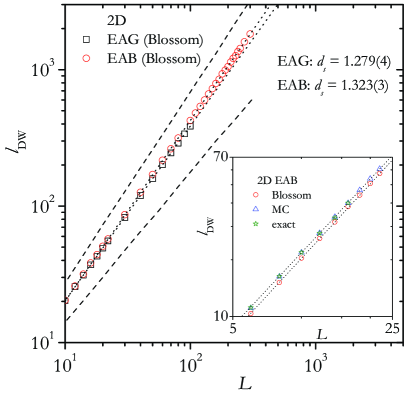
Studying systems of sizes up to the value that we estimate for the fractal dimension of the 2D EAB model is . This value is between the bounds given in Ref. Melchert2007, and is compatible both with the value obtained for the case of fully periodic BCs, and with the most recent estimate calculated using the entropy ansatz: . Aromsawa2007 Even though a value of has been reported previously, Roma2007 the small discrepancy with the value reported in this letter is due to the larger system sizes that are considered here (up to in Ref. Roma2007, ). For the sake of comparison, we have also calculated the fractal dimension for the 2D EAG. We obtain , which is compatible with the most recent and accurate value reported: . Melchert2007
Notice that the fractal dimensions obtained for the 2D EAB and the 2D EAG are clearly different. To check that this is not an artifact of the scaling function used to fit the points, , we have also tried fits with two other scaling functions with additional correction terms (see Table III). For EAB we have obtained for all the fits with and for periodic-free and periodic-periodic systems, respectively (a fit with is considered as a good fit numerical ). This shows that, with a high probability, the difference found between the fractal dimensions for the EAB and the EAG is not an effect of finite size scaling. This difference is further evidence that the universality of both models is different for .
| periodic-periodic BCs | periodic-free BCs | |||||||
|---|---|---|---|---|---|---|---|---|
As mentioned above, Eq. (1) (considering ) predicts . This is the same universality class as the loop-erased random walks. Schramm2000 Interestingly, the fractal dimension we obtain is much closer to , which is the fractal dimension of the normal self-avoiding walks. Flory This does not necessarily mean that DWs cannot be described as SLE processes. The walks generated by these processes have many interesting properties. One way to see whether DWs can be described as SLE processes is to test whether they have some of these properties. Bernard2007
We have performed one such test in 2D. If DWs are described by an SLE process of diffusion constant , the probability that they pass to the right of a point with polar angle (measured from the starting point of the walk) is Schramm2001 :
| (2) |
where is the hypergeometric function. Notice that does not depend on the radial coordinate of the reference point. The result of this test is shown in Fig. 5. The points for the EAG are compatible with a diffusion constant , which is consistent with the value obtained by Bernard et al.. Bernard2007 In turn, this value is compatible with the relation . For the EAB the points obtained are far from the curve (upper curve in Fig. 5) that corresponds to (using . In fact, they are much closer to (lower curve in Fig. 5). Thus, unless finite size effects are very significant, this result shows that EAB DWs cannot be consistently described as SLE processes. It must be stressed that this test has been performed using the DWs calculated with the Blossom algorithm which means that, for the EAB, the GSs have not been sampled uniformly. Nevertheless, as the determination of the fractal dimension of the DWs does not seem to be affected by this bias, it is not unreasonable to assume that it also does not affect the outcome of the SLE test. We have only used the Blossom algorithm because, for this kind of tests, very large system sizes must be studied to obtain meaningful results.
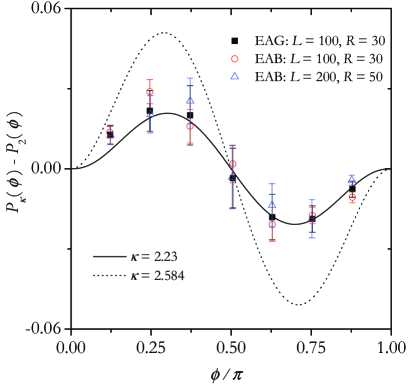
In conclusion, we have performed an extensive numerical study of the domain walls for the EAB and the EAG both in 2D and 3D, and have determined their fractal dimension from a direct measurement of their length. In 3D we find that both exponents coincide. On the other hand, for 2D systems we find a clear difference between the fractal dimensions of the EAB and the EAG. The value obtained for the EAB model shows that these domain walls are more similar to self-avoiding walks than to loop-erased random walks, as one would expect from Eq. (1). Even though the methods we have used do not sample uniformly the ground state space, the fact that all the obtained values of coincide is good evidence that this estimate must be very close to its true value: given the very different nature of the algorithms used it would be very unlikely that they give raise to the same wrong estimate of the fractal dimension. nota Finally we have tested whether the 2D EAB domain walls can be described by SLE processes. The outcome of this test is negative: the probability that a DW passes to the right of a given point is not consistent with an SLE process with .
This work has been supported by Universidad Nacional de San Luis (Argentina) under project 322000, CONICET (Argentina) under project PIP 6294 and the National Agency of Scientific and Technological Promotion (Argentina) under project 33328 PICT 2005.
References
- (1) S.F. Edwards and P.W. Anderson, J. Phys. F 5, 965 (1975).
- (2) C. Amoruso, E. Marinari, O. C. Martin, and A. Pagnani, Phys. Rev. Lett. 91, 087201 (2003).
- (3) A. K. Hartmann, cond-mat/0704.2748.
- (4) C. Amoruso, A. K. Hartmann, M. B. Hastings, and M. A. Moore, Phys. Rev. Lett. 97, 267202 (2006).
- (5) D. Bernard, P. Le Doussal, and A. A. Middleton, Phys. Rev. B 76, 020403(R) (2007).
- (6) A. K. Hartmann, A. J. Bray, A. C. Carter, M. A. Moore, and A. P. Young, Phys. Rev. B 66, 224401 (2002).
- (7) O. Melchert and A. K. Hartmann, Phys. Rev. B 76, 174411 (2007).
- (8) A. K. Hartmann and A. P. Young, Phys. Rev. B 64, 180404(R) (2001).
- (9) D. S. Fisher and D. A. Huse, Phys. Rev. Lett. 56, 1601 (1986).
- (10) L. Saul and M. Kardar, Phys. Rev. E 48, R3221 (1993).
- (11) A. Aromsawa and J. Poulter, Phys. Rev. B 76, 064427 (2007).
- (12) F. Romá, S. Risau-Gusman, A. J. Ramirez-Pastor, F. Nieto, and E. E. Vogel, Phys. Rev. B 75, 020402(R) (2007).
- (13) M. Weigel and D. Johnston, Phys. Rev. B 76, 054408 (2007).
- (14) Notice that in 2D the bonds in the lattice correspond to bonds in its dual lattice, but in 3D they correspond to plaquettes.
- (15) J. Hoshen and R. Kopelman, Phys. Rev. B 14, 3438 (1976).
- (16) A. Hartwig, F. Daske, and S. Kobe, Comput. Phys. Commun. 32, 133 (1984).
- (17) J. W. Landry and S. N. Coppersmith, Phys. Rev. B 65, 134404 (2002).
- (18) K. Hukushima and K. Nemoto, J. Phys. Soc. Jpn. 65, 1604 (1996).
- (19) N. Metropolis, A. W. Rosenbluth, N. M. Rosenbluth, A. H. Teller, and E. Teller, J. Chem. Phys. 21, 1087 (1953).
- (20) C. De Simone, M. Diehl, M. Jünger, P. Mutzel, G. Reinelt, and G. Rinaldi, J. Stat. Phys. 80, 487 (1995); J. Stat. Phys. 84, 1363 (1996).
- (21) We have used the spin-glass ground-state server of the University of Cologne where a branch-and-cut algorithm is available online, http://www.informatik.uni-koeln.de/lsjuenger/index.html.
- (22) F. Romá, S. Risau-Gusman, A. J. Ramirez-Pastor, F. Nieto, and E. E. Vogel, in preparation.
- (23) M. Cieplak and J. R. Banavar, J. Phys. A. 23, 4385 (1990).
- (24) M. Palassini and A. P. Young, Phys. Rev. Lett. 83, 5126 (1999).
- (25) T. Aspelmeier, A. J. Bray, and M. A. Moore, Phys. Rev. Lett. 89, 197202 (2002).
- (26) M. Palassini, F. Liers, M. Jünger, and A. P. Young, Phys. Rev. B 68, 064413 (2003).
- (27) A. K. Hartmann and A. P. Young, Phys. Rev. B 66 094419 (2002).
- (28) A. K. Hartmann and H. Rieger, Optimization Algorithms in Physics (Wiley-VCH, Berlin, 2001).
- (29) W. J. Cook and A. Rohe, INFORMS J. Comput. 11, 138 (1999).
- (30) J. W. Landry and S. N. Coppersmith, Phys. Rev. B 65, 134404 (2002).
- (31) W. H. Press, S. A. Teukolsky, W. T. Vetterling, and B. P. Flannery, Numerical Recipes in C (Cambridge University Press, 1992).
- (32) O. Schramm, Isr. J. Math 118, 221 (2000).
- (33) P. J. Flory, Principles of Polymer Chemistry (Cornell University Press, Ithaca NY, 1953).
- (34) O. Schramm, Electron. Commun. Probab. 6, 115 (2001).
- (35) Of course, one cannot exclude the possibility that there exists an algorithm whose ground state sampling is so much biased that it gives a different value of the slope of the fit.