PRINCIPAL COMPONENT ANALYSIS OF THE TIME- AND POSITION-DEPENDENT POINT SPREAD FUNCTION OF THE ADVANCED CAMERA FOR SURVEYS
Abstract
We describe the time- and position-dependent point spread function (PSF) variation of the Wide Field Channel (WFC) of the Advanced Camera for Surveys (ACS) with the principal component analysis (PCA) technique. The time-dependent change is caused by the temporal variation of the focus whereas the position-dependent PSF variation in ACS/WFC at a given focus is mainly the result of changes in aberrations and charge diffusion across the detector, which appear as position-dependent changes in elongation of the astigmatic core and blurring of the PSF, respectively. Using archival images of star cluster fields, we construct a ACS PSF library covering diverse environments of the observations (e.g., focus values). We find that interpolation of a small number () of principal components or “eigen-PSFs” per exposure can robustly reproduce the observed variation of the ellipticity and size of the PSF. Our primary interest in this investigation is the application of this PSF library to precision weak-lensing analyses, where accurate knowledge of the instrument’s PSF is crucial. However, the high-fidelity of the model judged from the nice agreement with observed PSFs suggests that the model is potentially also useful in other applications such as crowded field stellar photometry, galaxy profile fitting, AGN studies, etc., which similarly demand a fair knowledge of the PSFs at objects’ locations. Our PSF models, applicable to any WFC image rectified with the Lanczos3 kernel, are publicly available.
1 INTRODUCTION
Even in the absence of atmospheric turbulence, the finite aperture of Hubble Space Telescope () causes light from a point source to spread at the focal plane with the diffraction pattern mainly reflecting the telescope’s aperture and optical path difference function. Although the point-spread-function (PSF) of is already far smaller than what one can achieve with any of the current ground-based facilities, astronomers’ endless efforts to push to the limits of their scientific observations with ever increase the demand for the better knowledge of the instrument’s PSF. Especially, since the installation of the Advanced Camera for Surveys (ACS) on , there have been concentrated efforts to carefully monitor and understand the instrument’s PSFs, and to utilize the unparalleled resolution and sensitivity of ACS in gravitational weak-lensing (e.g., Jee et al. 2005a; Heymans et al. 2005; Schrabback et al. 2007; Rhodes et al. 2007).
Modeling the PSFs of ACS has proven to be non-trivial because of its complicated time- and position-dependent variation. The time-dependent change occurs due to the variation in the focus, which relates to the constant shrinking of the secondary mirror truss structure and the thermal breathing of . The former is the main cause of the long-term focus change, and the secondary mirror position has been occasionally adjusted to compensate for this shrinkage (Hershey 1997). The latter is responsible for the short-term variation of the focus and is affected by the instrument’s earth heating, sun angle, prior pointing history, roll angle, etc. Even at a fixed focus value of , the PSFs of ACS also significantly change across the detector from the variation of the CCD thickness and the focal plane errors, which appear as position-dependent changes in charge diffusion and elongation of the astigmatic cores, respectively.
The strategies to model these PSF variations can be categorized into two types: an empirical approach based on real stellar field observations and a theoretical prediction based on the understanding of the instrument’s optics. The first method treats the optical system of the instrument nearly as a blackbox and mainly draws information from observed stellar images. Although the PSF variation pattern can be most straightforwardly described by the variation of the pixel intensity as a function of position (e.g., Anderson & King 2006), frequently orthogonal expansion of the observed PSFs (e.g., Lauer 2002; Bernstein & Jarvis 2002; Refregier 2003) have been utilized to make the description compact and tractable. On the other hand, the second approach mainly relies on the careful analysis of the optical configurations of the instrument and receives feedbacks from observations to fine-tune the existing optics model. The TinyTim software (Krist 2001) is the unique package of this type applicable to most instruments of .
In this paper, we extend our previous efforts of the first kind (Jee et al. 2005a; 2005b; 2006; 2007) to describe the time- and position-dependent PSF variations of ACS/WFC now with the principal component analysis (PCA). In our previous work, we used “shapelets” (Bernstein & Jarvis 2002; Refregier 2003) to perform orthogonal expansion of the PSFs. Shapelets are the polar eigenfunctions of two-dimensional quantum harmonic oscillators, which form a highly localized orthogonal set. Although the decomposition of the stars with shapelets is relatively efficient and has proven to meet the desired accuracy for cluster weak-lensing analyses, the scheme is less than ideal in some cases. One important shortcoming is that it is too localized to capture the extended features of PSFs (Jee et al. 2007; also see §2.1). In principle, the orthonormal nature of shapelets should allow us to represent virtually all the features of the target image when the number of basis functions are sufficiently large. However, this is not a viable solution not only because the convergence is slow, but also because the orthonormality breaks down in pixelated images for high orders as the function becomes highly oscillatory within a pixel.
The PCA technique provides us with a powerful scheme to obtain the optimal set of basis functions from the data themselves. Unlike “shapelets”, the basis functions derived from the PCA are by nature non-parametric, discrete, and highly customized for the given dataset. Therefore, it is possible to summarize the multi-variate statistics, with a significantly small number of basis functions (i.e., much smaller than the dimension of the problem). For example, PCA has been applied to the classification of object spectra in large area surveys (Connolly et al. 1995; Bromley et al. 1998; Madgwick et al. 2003). It has been shown that only a small number () of the basis functions or are needed to reconstruct the sample. The application of PCA to the PSF decomposition is used by the Sloan Digital Sky Survey (SDSS) to model the PSF variations (e.g., Lupton et al. 2001; Lauer 2002). Jarvis & Jain (2004) used the PCA technique to describe the variation in the PSF pattern in the CTIO 75 square-degree survey for cosmic shear analyses. They fit the “rounding” kernel component with PCA, not the PSF shape directly. This scheme is motivated by their shear measurement technique (i.e., reconvolution to remove systematic PSF anisotropy). However, in the current study we choose to fit the PSF shapes directly because this is more general in the sense that the rounding kernel components are not uniquely determined for a given PSF. In addition, our PSF library generating the PSF shapes directly has more uses in other studies.
We aim to construct a high-quality PSF library for the broadband ACS filters (F435W, F475W, F555W, F606W, F625W, F775W, F814W, and F850LP) from archival stellar images, which sample a wide range of the environments (e.g., the focus values). Our PSF models describe ACS PSFs in rectified images, specifically, drizzled using the Lanczos3 kernel with an output pixel scale of 0.05″(see §4.1 for the justification of this choice). The results from this work are made publicly available on-line via the ACS team web site111The full PSF library of ACS will become available at http://acs.pha.jhu.edu/mkjee/acs_psf/..
We will present our works as follows. The justification and the basic mathematical formalism of PCA are briefed in §2. In §3, we demonstrate how the technique can be applied to ACS data with some test results. Focus dependency of the ACS PSFs, comparison with TinyTim, and strategies to find matching templates are discussed in §4 before we conclude in §5.
2 PRINCIPAL COMPONENT ANALYSIS OF POINT SPREAD FUNCTIONS
2.1 Optimal Basis Functions for Modeling a PSF Variation
The concept that any vector in a vector space can be represented as a linear combination of the orthonormal basis vectors can be easily extended to a two-dimensional image analysis. The most natural set of basis vectors for a resolution image is a set of unit vectors, where the unit vector represents the Cartesian coordinate axis in the dimension; the pixel value represents the amplitude along the axis. These unit vectors form the most intuitive set of orthonormal vectors and are in fact still a popular choice for describing a variation especially when the dimension is low. For larger images, however, it is obvious that one needs to find alternative basis vectors, which can describe the image features and their variations more compactly with less number of basis vectors than . In the following, we will briefly review our experiments with two potentially useful methods, namely wavelet and shapelet decomposition schemes in an attempt to compactly model PSF features. By discussing some fundamental limits of these two approaches, we will justify the need for the new scheme, PCA, to overcome these pitfalls.
In astronomy, a analysis has been among the most popular choices in compressing object images, identifying objects, recognizing patterns, filtering noise, etc. The method has significant advantages over a traditional Fourier method particularly when the signal contains discontinuities and sharp spikes. Wavelets refer to finite and fast-decaying orthogonal basis functions, which can efficiently represent localized signals. Because PSFs are in general compact, sharp, and localized, the wavelet transform can be considered as a tool for describing the PSF and its variation. However, we find that, although the scheme is very powerful in representing the global feature, the wavelet representation with a small subset of the entire basis functions cannot fully capture the sophisticated details of a ACS PSF. Shown in Figure 1b is a wavelet representation of the ACS/WFC PSF (Figure 1a) with % (157 out of 961) of the total basis vectors retained. The PSF core within pixel radius is satisfactory whereas most of other features beyond pixel radius are severely smeared. Although it is possible to improve the quality of the wavelet representation by employing more basis functions, we observe that the convergence is slow and one has to include more than % of the entire basis functions to achieve the goal.
Bernstein & Jarvis (2002) and Refregier (2003) proposed to use shapelets to decompose astronomical objects. Shapelets, also forming an orthogonal set, are derived from Gaussian-weighted Hermite polynomials, which are eigenfunctions of two-dimensional quantum harmonic oscillators. As shapelets are based on two dimensional circular Gaussian functions, they are somewhat more localized than , thus potentially more efficient in describing the PSF core. Figure 1c shows that indeed the central region of the PSF is nicely recovered with 78 basis functions (shapelet order of 12); the second diffraction ring at pixels is clear. It is not surprising however to observe that the other features beyond pixels are completely washed out in Figure 1c because the Gaussian nature of the shapelets truncates the profile too early to capture the apparent PSF wings. The fraction of the flux distributed outside the second diffraction ring is less than 5 % (compared to the original 3131 PSF) and thus is negligible for some applications. In particular, if one looks for lensing signals in galaxy clusters, the inaccuracy in shear measurement caused by this PSF wing truncation is overwhelmed by the shear-induced ellipticity changes. However, in modern cosmic shear studies, the required level of systematic errors are much more stringent, and thus we still want to develop an even better scheme that robustly describes the PSF features on both small and large scales.
From the above two experiments, it becomes clear that any basis functions that are derived from some analytic functions have fundamental limits in their efficiency when we require both small and large scale features (i.e., central cuspiness and extended diffraction pattern) of PSFs to be stringently recovered. This implies that the ideal basis functions for a given dataset must be derived from the dataset itself. One powerful method to achieve such a goal is PCA. Also known as Karhunen-Loeve transformation (KLT), PCA provides a method for obtaining optimal basis functions highly tailored to a given problem. As will be briefly summarized in §2.2, PCA allows us to keep the subset of basis functions that has the largest variance. The principal components (hereafter we use the terms, principal component, basis function, and eigen-PSF interchangeably) with the lowest variances are dominated by noise and can be safely discarded to reduce the dimension of the problem.
We display the PSF image constructed with the first 20 principal components in Figure 1d. The 20 principal components are obtained by analyzing stars in the same exposure. The dramatic improvement in the recovery of the original PSF is apparent not only in the core, but also in the diffraction pattern far from the core. This is again verified in the comparison of the radial profiles in different representation of the PSF (Figure 2). The PCA method gives the radial profile closest to that of the original (we note that the PCA method slightly fits noise at because the signal outside the second diffraction ring is very weak. Potentially one can improve the sampling by including the wings of saturated stars as is done by Anderson & King [2006]). The shapelet method generates the PSF that truncates at pixels. The representation with 150 wavelets appears to approximate the radial profile of the original closely, but we see in Figure 1 that the two-dimensional representation is unacceptable. Therefore, considering both the relatively small number of basis functions and the quality of the reproduction, we choose the PCA approach for our subsequent analysis of the time- and position-dependent PSF of WFC.
2.2 Mathematical Formalism
Imagine that we have a dataset consisting of observations (e.g., stars), each with observable properties (e.g., pixel values). If the observable properties do not change greatly between observations, the dataset forms a cloud of points in an -dimensional space. We want to construct a set of () orthonormal vectors that describes the subspace in the following manner.
-
•
The first significant vector is defined as the axis with a minimal mean distance from each point.
-
•
The second significant vector is orthogonal to the first significant vector and minimizes the mean distance from each point.
-
•
The significant vector is orthogonal to the previous significant vectors and minimizes the mean distance.
These significant vectors are called principal components (PC) of the system.
One way to construct such a new orthonormal basis is Singular Value Decomposition (SVD; Press et al. 1992). We can express the above dataset as a matrix S. According to the SVD theory, any matrix whose number of rows is greater than or equal to its number of columns , can be rewritten as the product of an column-orthogonal matrix U, an diagonal matrix W with positive or zero elements, and the transpose of an orthogonal matrix V
| (1) |
It is easy to show that once the matrix S is expanded in the way above, any element of the matrix S can be reconstructed by
| (2) |
Equation 2 helps us to realize that, if some of the singular values (elements of W) are tiny, we can approximate the matrix S by replacing those small ’s with zeros. This effectively reduces the number of columns in U and V. The remaining columns of V serve as the principal components that form an orthonormal basis.
A geometric meaning of these principal components is that they define the principal axes of the error ellipsoid. Consequently, they are eigenvectors of the covariance matrix of the dataset C, diagonalizing C with eigenvalues of , which also illustrates that PCA is the rotation of the system into a new basis (i.e., principal components) to describe the data in terms of statistically independent quantities.
In practice, PCA necessitates preprocessing of the data typically involving mean subtraction and normalization. The exact procedure highly depends on the statistical nature of the problem and we will discuss the issues in §3.1.
3 PCA APPLICATION TO ACS DATA
3.1 Implementation
In the current section, we demonstrate how we can describe the PSF variation observed in a single ACS/WFC exposure with PCA described in §2.2. We select the F814W observation of the 47 Tuc field taken on 6 May 2002 in two 30s exposures (dataset ID = J8C0D1051). The image was part of a series of observations to derive flat-fielding model of the instrument (PROP ID 9018). The low level CCD processing was carried out using the STScI standard ACS calibration pipeline (CALACS; Hack et al. 2003). In correcting the geometric distortion, we used a Lanczos3 drizzling kernel with an output pixel size of 0.05. In our previous analyses (Jee et al. 2005a; 2005b; 2006; 2007), this combination of drizzling parameters has been verified to be among the optimal choices in minimizing the aliasing, the noise correlation, and the broadening of the PSF. We discuss some important differences arising from different choices of drizzling parameters in §4.1.
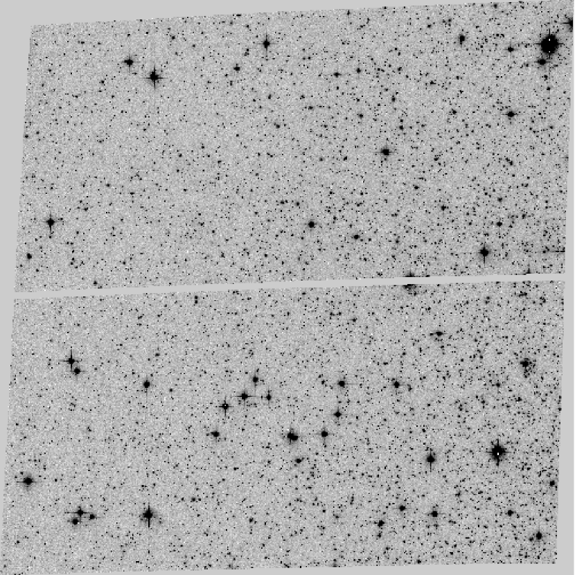
The field is moderately crowded (Figure 3) and we were able to select bright (), unsaturated, and isolated (no adjacent stars within a pixel radius) stars. After creating a postage stamp image ( pixel pixel) for each star, we applied sub-pixel shifts so that the peak always lies on the center of a pixel. Omitting this procedure would result in the variance of the system largely dominated by the location of the peaks within pixels. The sub-pixel shifts were carried out with bicubic interpolation, which closely approximates the theoretically optimal, windowed sinc interpolation by cubic polynomials. We find that although bicubic interpolation slightly softens PSF cores relative to the results from windowed sinc interpolation, the latter creates more frequent other types of artifacts such as occasional negative pixels (in theory, the sinc interpolant is valid for a Nyquist-sampled image).
We need to express the PSF images with one-dimensional vectors. Because the modeling size is , each vector has 961 elements. Our matrix S describing the dataset has columns and rows. There are more columns than rows, and the SVD above will yield (or more because of the degeneracies) zero or negligible ’s. However, the remaining V still contains useful principal components of the system, which can efficiently represent the sample.
We normalized S in such a way that the sum of the elements in each row is unity after subtracting the background value (flux normalization). Next, we created a mean PSF by taking averages along the columns. Then, we subtracted this mean PSF from each row. The resulting matrix S consists of deviations from this mean PSF.
We perform SVD of S by diagonalizing the covariance matrix C, which is the outer product of S with itself. The resulting eigenvectors and the eigenvalues are the PCs and the variances of the matrix, respectively. Finally, we sort the result in order of decreasing variances. Figure 4 illustrates that the first PCs account for more than 90% of the total variance. Each of the remaining 900 principal components is responsible for less than 1% of the total, likely to be associated with noise rather than to contain the real signal.
We determined the PC coefficients (i.e., amplitudes along the eigenvectors) down to the 20th largest component by multiplying S to the eigenvectors for the selected stars. The spatial variation of each coefficient is fit with the following polynomial:
| (3) |
We found that a fifth order in (i.e. ) is sufficient to describe the pattern and higher order polynomials do not improve (sometimes worsen) the agreement between model and data. The total number of coefficients necessary to model the PSF variation for a entire WFC frame is .
3.2 Test Results
There might exist a number of ways to compare our PSF model obtained in §3.1 with the real PSFs, depending on how one chooses to characterizes PSFs. In this paper, we characterize PSFs by their ellipticity and width because these parameters are natively related to the systematics in weak-lensing measurements and also are sensitive to the charge diffusion and the local focus offset.
We measure a star’s ellipticity and width using the following quadrupole moments,
| (4) |
where is the pixel intensity at , is the center of the star, and is the weight function required to suppress the noise in the outskirts (we choose a Gaussian with a FWHM of 2 pixels throughout the paper). With Equation 4 at hand, it is now possible to define the star’s ellipticity in the following two ways:
| (5) |
and
| (6) |
For an ellipse with axis ratio , and correspond to and , respectively. In the current paper, we select Equation 6 as our definition of ellipticity, referring to the first and second components of as and , respectively. The size of a star can be similarly defined using the above quadrupole moments . One common choice is
| (7) |
which we adopt in this work.
In the left panel of Figure 5, we display the ellipticities of the isolated stars found in Figure 3. The size and the orientation of the “whiskers” represent the magnitude of ellipticity and the direction of elongation, respectively. The majority of the stars are stretched approximately parallel to the line. This direction is roughly tangential to the vector pointing towards the telescope axis, and this type of pattern is observed when is at its nominal “negative” focus (the actual focus offsets on the surface of the WFC detector can be positive in certain regions because of the curvature of the focal plane and the detector height variation). We repeat this ellipticity measurement for our model PSFs and the results are shown in the middle panel of Figure 5, which displays the predicted ellipticities of PSFs at the same star positions. We plot the residual ellipticities in the right panel. It is apparent that our PSF model obtained through PCA robustly recovers the observed ellipticities. With 3 outliers discarded, the mean absolute deviation is , and the mean ellipticity is .
Another way to quantify the quality of the ellipticity representation of a PSF model is to investigate the ellipticity correlation as a function of separation :
| (8) |
and
| (9) |
We show in Figure 6 the ellipticity correlation functions for the the observed PSF (left), the model (middle), and the residual (right). The solid and dash lines represent and , respectively. The amplitude of the residual ellipticity correlation is (after discarding the values at , which are spuriously high due to the poor statistics in this regime and an artifact of the interpolation), approximately three orders of magnitude lower than the uncorrected values.
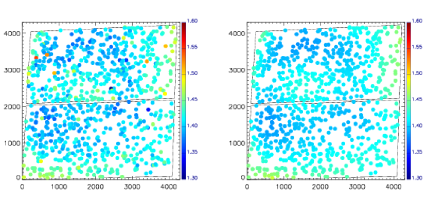
A size of the PSFs (eqn. 7) is also a useful quantify in characterizing PSFs. In general, both the aberration-induced elongation and the charge diffusion are responsible for the broadening of WFC PSFs. Krist (2003) noticed that the PSF width variation by charge diffusion remarkably resembles the pattern of the WFC CCD thickness variation. The blurring is most severe in the central region where the CCD layer is the thickest, and the annulus surrounding this region has the least charge diffusion, consistent with its lowest thickness. The left panel of Figure 7 shows our estimation of the position-dependent WFC PSF width variation measured from the stars in Figure 3. The global pattern nicely agrees with the result of Krist (2003) (i.e., the detection of the “hill” at and and the “moat” surrounding the hill). Because the image is taken in F814W, the charge diffusion effect is somewhat reduced (compare this with Figure 2 of Krist 2003 showing the variation in F550M). In addition, we note that the PSF widths are greatest along the field boundary, which is by and large due to the optically induced PSF elongation. We display the PSF width variation predicted from our model in the right panel of Figure 7. The employed polynomial interpolation smooths the variation and slightly flattens the “hill” and “moat” features. The stars in the hill in the right panel are % smaller whereas the stars in the moat are % larger.
Krist (2003) claimed that there was a height difference of between the two CCDs, which manifested itself as a discontinuity of the PSF pattern across the gap. The observed PSF size variation (left panel of Figure 7) seems to show faint indications of the height difference. However, we do not find any noticeable discontinuity in the PSF ellipticity pattern across the gap in Figure 5.
4 DISCUSSION
4.1 Effects of Drizzling Methods on PSF Characteristics
Aliasing occurs when a signal that is continuous in space is sampled with finite resolution. PSF shapes from rectified ACS images suffer this aliasing twice, first when photons are collected in the discrete CCD grid, and second when the raw data are remeshed for the geometric distortion correction. Dithering mainly helps to reduce the first aliasing by changing the sub-pixel position of the PSF centers within a pixel, effectively increasing the sampling resolution of the detector beyond its physical pixel size. The second aliasing arising from the input and output pixel offsets is mitigated by carefully selecting an interpolation scheme. Here, we focus on the second issue: the relation between interpolation scheme (i.e., parameters set in drizzling) and observed PSF characteristics.
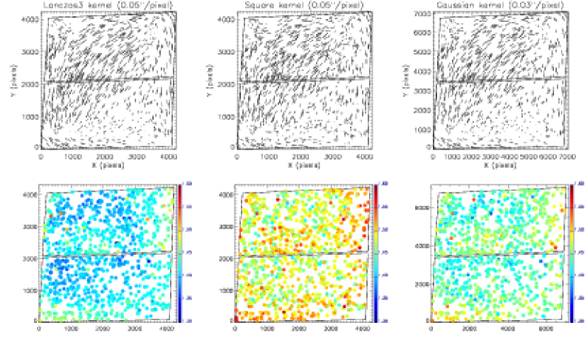
Although quite a few combinations of drizzling kernels, output pixel sizes, and drop sizes are possible, we consider the following three cases:
-
•
Lanczos3 kernel, output pixel, and pixfrac,
-
•
Square kernel, output pixel, and pixfrac, and
-
•
Gaussian Kernel, output pixel, and pixfrac.
The first case is of course the choice in the current paper. The second case is selected because it is the default setting in the STScI pipeline and is most frequently used. The last one is favored by Rhodes et al. (2007), who argued that this combination gave the minimal aliasing in their experiments.
We compare the results from these three methods by examining the PSF ellipticity and width distribution across the WFC detector (Figure 8). As noted by Rhodes et al. (2007), it is obvious that drizzling with square kernel and 0.05 output pixel produces the most severe aliasing among the three. The residuals between the observed (top middle) and the PCA interpolated stars (as calculated in the second panel of Figure 5) have a mean absolute deviation of with a center at . In addition, the PSF blurring is also the largest ( ) in the square-kernel-drizzled image. The mean PSF width is , about 5.4% larger than the value we obtain from the Lanczos3-kernel-drizzled image ().
Drizzling with a Gaussian kernel with a pixel scale of 0.03 ( ) reduces the aliasing in the ellipticity measurements compared to that in the square kernel image. The residuals have a mean absolute deviation of with a center at . However, the mean absolute deviation is % higher than in the Lanczos3 case. Also, although it is true that the PSF broadening is mitigated compared to the square-kernel drizzling, the mean PSF width () is % larger than the Lanczos3-kernel PSF width.
Based on the above experiment, we claim that the Lanczos3 kernel with an output pixel size of 0.05 should be a preferred choice in weak-lensing analyses (and also perhaps in other analyses that require sharpest images). Although the choice of the Gaussian kernel with a pixel scale of 0.03″provides a competitive performance in terms of the reduction of aliasing and the sharpness of PSF, we have observed that noise correlation is the most severe in this case (this pitfall is also noted by Rhodes et al. [2007]). Noise correlation between adjacent pixels creates visible moiré patterns in the image.
However, we comment that the Lanczos3 kernel occasionally produces some cosmetic artifacts in the region where flux gradients change abruptly (e.g., centers of saturated stars, wings of bright stars, missing data points, etc.). Nevertheless, these occasional cosmetic artifacts in individual stars are not of concern in the current PSF sampling because they are efficiently filtered out through PCA.
4.2 Focus Dependency
In §3.2, we studied how the ellipticity and the size of WFC PSFs vary across the field for the particular dataset (the F814W filter on 19 April 2002). If the pattern remained the same throughout the life of or if the change were negligible, the issue of correcting PSF effects would be trivial. Unfortunately, an observed PSF pattern is not stable, but changes over time, depending largely on the focus status of . The main cause of the focus variation is the combination of both the constant shrinkage and the thermal breathing of the optical telescope assembly (OTA) truss structure. Occasional adjustments of the secondary mirror position were applied (e.g., on 24 December 2004) to compensate for the former long-term change. The latter thermal breathing occurs as the OTA truss structure expands during Earth occultation and contracts after the occultation. The typical amplitude of the focus change during an orbit is . This small focus variation does not severely affect the quality of ACS observations in general. However, it produces conspicuous changes in the PSF ellipticity and width variation across the detector.
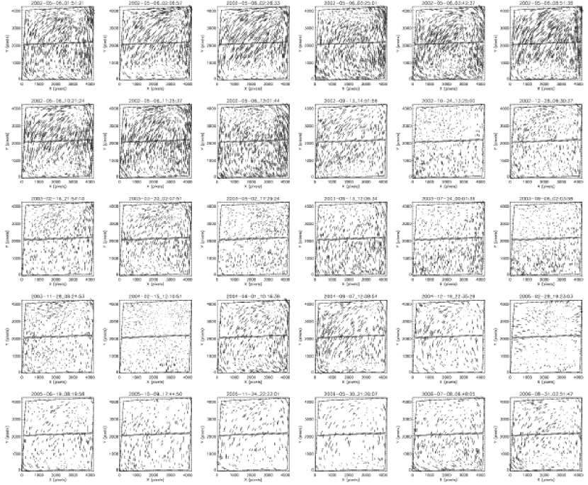
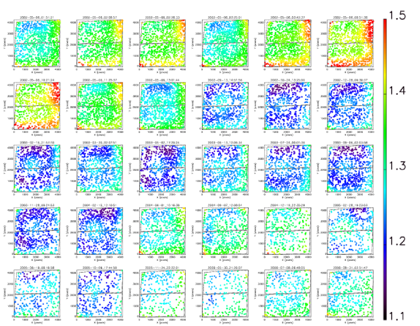
In Figure 9 and 10, we show the time-dependent PSF pattern in ellipticity and width, respectively, observed in 30 different F435W exposures. In both figures, time increases to the right and to the bottom; the observation date and time are denoted in the and (UT) format above each panel. The exposures are not homogeneously sampled in time (e.g., the first 9 exposures are taken on the same observation date). It is clear that the PSF ellipticity and width patterns vary quite significantly. When the instrument is at negative focus, the “whiskers” are on average elongated from lower left to upper right as already seen for the case in §3.2. We observe that these negative focus patterns dominate over positive focus patterns not only in F435W, but also in other filter observations. At positive focus, the whiskers are approximately perpendicular to the pattern observed at negative focus (e.g., plots in the fourth row of the second and the sixth columns). Comparison between Figure 9 and 10 show that the average PSF widths per pointing are in general proportional to the average magnitudes of ellipticities (i.e., size of whiskers). Moreover, we realize that the PSF width variation pattern is potentially a more sensitive measure of the HST focus and helps us to characterize the pattern more precisely. For example, the first 9 exposures taken on the same observation date appear to possess ellipticity patterns very similar to one another. If one is somehow asked to select two PSF patterns that were observed under similar circumstances, the task based on the visual inspection of these ellipticity plots is quite challenging. However, with the aid of Figure 10 one can easily tell that the first one can pair with the fourth one, the second one with the third one, the sixth one with the seventh one, etc.
A close examination of the time-dependent variation of the pattern suggests that the patterns are repeatable even if their observation epochs are quite apart. For example, the two observations taken on 24 October 2002 (2nd row and 5th column) and 6 September 2003 (3rd row and 6th column) match each other not only in the ellipticity pattern, but also in the PSF width pattern. Although this repeatability does not necessarily guarantee that the PSF pattern is uniquely determined by a single parameter (focus), it provides important justification that we can apply the PSF templates obtained from these stellar fields to science observations taken at different epochs.
We suspect that other factors such as velocity aberration, detector plane tilt, pointing accuracy degradation, etc. also might modulate the observed pattern. As suggested by Jarvis & Jain (2006), PCA of the polynomial coefficients may help us to determine the number of degrees of freedom in future investigations.
4.3 Comparison with a shapelet approach
In our previous studies, we used shapelets to interpolate PSF variations across WFC. Although shapelets provide competitive efficiency in describing ACS PSFs, their performance is somewhat inferior to the current method obviously because the basis functions derived from PCA is optimally customized to the given data. In the following, we present quantitative comparison using the same dataset (J8C0D1051) analyzed with PCA in §3.1.
We choose a shapelet order to be eight and apply a 4th order polynomial interpolation. As stated in Jee et al. (2005a), increasing the order of polynomials beyond the third order does not improve the fit. A shapelet order of eight contains 45 independent basis functions. We again emphasize that increasing the order of shapelet beyond this at the expense of computation time does not noticeably improve the quality of the ACS PSF representation (sometimes this makes the interpolation unstable as the high order terms start fitting the noise).
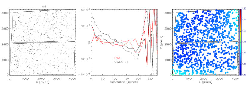
The left panel of Figure 11 shows the ellipticity residuals between the observed stars and the shapelet model. The mean absolute deviation is after 3 outlier rejection. This is very close to the value that we obtained from the PCA method (). However, the residual ellipticity correlation (middle panel of Figure 11) illustrates that the systematic errors of the shapelet model (black) is somewhat higher than the PCA model (red); we see higher correlation on small scales () and higher anti-correlation on large scales ().
In the right panel of Figure 11, we display the ACS PSF width variation predicted by the shapelet model. Comparison of this plot with Figure 7 shows that the shapelet model dampens the variation pattern. The “moat” and “hill” features are hard to identify although the model satisfactorily describes the broadening at the field boundaries (the lower-right and upper-right corners). We note that the widths of “hill” stars here are % smaller than those of the observed stars.
In summary, the ACS PSF variation model through shapelet coefficient interpolation performs competitively well in representing the ellipticities although we note that the systematics in the shapelet PSF model is higher than in the PCA PSF model. The shapelet PSF model does not fully describe the ACS PSF width variation, under-representing the “moat” and “hill’ features. These shortcomings are not worrisome in typical cluster weak-lensing analyses, where the residual systematics are still far smaller than galaxy shape or foreground-contamination noise. However, the under-representation of the PSF widths makes the shapelet model inadequate for some applications (e.g., precision stellar photometry, cosmic shear measurement, etc.); in particular, the PSF width variation is directly related to shear calibration (dilution correction) biases of cosmic shear measurements.
4.4 Comparison with TinyTim
TinyTim is a software package for generating simulated PSFs for various instruments installed on . The diffraction pattern is modeled by careful understanding of the telescope’s aperture and the optical path difference functions. Because the current publicly available version of TinyTim is also capable of modeling field-dependent variations in aberrations and charge diffusion for a full set of ACS filters at different focus offsets, in principle it can obviate our empirical efforts to model PSFs the results are consistent with stellar observations.
In order to compare TinyTim PSFs with those of real observations, we generated PSF templates with TinyTim by varying focus values and star positions. We changed the focus values at the interval from to , and for a given focus we placed stars at the pixel interval, uniformly covering the WFC detector. Because the final products by TinyTim are the ACS PSFs in a distorted frame, we applied drizzle with the Lanczos3 kernel (the choice that we also made for the observation) to simulate the geometric distortion correction effect.
We determined the “focus” of the observation in Figure 3 to be by searching for the TinyTim PSF template that best matched the observed ellipticity variation (shown in the left panel of Figure 5). The first panel of Figure 12 shows the ellipticity pattern for the observation predicted by TinyTim. Comparison with the left panel of Figure 5 gives a visual impression that TinyTim PSFs can reproduce the global feature of the ACS PSF variation. However, when examined star-by-star, the TinyTim PSFs give large systematic residuals (second panel); in general TinyTim stars appear to have more vertical elongation (i.e., smaller ). Obviously, these large systematic residuals translate into the high amplitudes of ellipticity correlations (third panel). The PSF width variation (fourth panel) predicted by TinyTim closely resembles the observed pattern (see Figure 7 for comparison). We note, however, that the PSF widths of the TinyTim stars are systematically smaller (%) than the observed values.
The large systematic residuals in ellipticity are worrisome. This non-negligible discrepancy between the TinyTim prediction and the observation suggests that TinyTim ACS PSFs cannot be directly applied to ACS observations if PSF anisotropy is of critical concern. For example, most weak-lensing studies draw lensing signal from faint, small galaxies that are only slightly larger than instrument PSFs. The large residual ellipticities shown in Figure 12 can mimic (false) lensing signals.
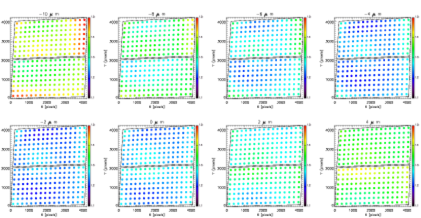
Of course, this TinyTim vs. observation mismatch is not confined to this particular observation (J8C0D1051). To compare with the observed PSF patterns presented in Figure 9 and 10 for F435W, we generate TinyTim PSF ellipticities of the same filter for the focus values ranging from -10 m to m in Figure 13 and 14. Again, we emphasize that the TinyTim PSFs reproduce the global feature of the PSF variation; as described by Krist (2003), we note that at negative focus values, the PSFs are on average elongated from lower-left to upper-right and at positive focus values the average elongation rotates by 90°. However, a scrutiny reveals that on small scales there exist some important discrepancies similar to the ones already demonstrated in Figure 12
One additional discrepancy deserving our attention is the feature near the gap between the two CCDs. A conspicuous discontinuity in ellipticity is observed in the TinyTim predictions (especially from the focus offset of m to m) whereas in the observed PSFs the ellipticity change across the gap appears to be continuous. The discontinuity appears because the TinyTim assumes that there is a height offset of between WFC1 and WFC2 based on the previous focus-monitoring program results (Krist 2003). Rhodes et al. (2007) also noticed this discrepancy between the observed stars in the COSMOS field and the TinyTim model stars, and attributed the absence of this discontinuity across the chip in observations to CTE degradations. This is a plausible explanation considering that the CTE-induced charge trailing in Y-axis can cause an increase in PSF ellipticity along the same direction; the regions near the chip gap are farthest from the readout registers and thus are subject to greatest charge trailing. Because Rhodes et al. (2007) relied on TinyTim for the correction of PSF effects in the COSMOS field, they introduced some empirical multiplicative factors to their quadrupole moment measurements in order to improve the agreement between TinyTim and COSMOS field stars.
However, although we observe that in certain situations the CTE degradation can lead to some smearing of PSFs in direction, we attribute the TinyTim and the observation mismatch largely to the imperfection of TinyTim rather than to the imperfection of the CCDs (i.e., CTE degradation) based on the following points. First, such discontinuities as predicted by TinyTim are absent or negligibly small in real observations not only in the latest data, but also in the earliest data soon collected after the installation of ACS on Hubble in March 2002. The CTE degradation is mainly caused by exposure to high-energy charged particles in the space environment, and thus the degradation grows with time. If the effect of the CTE degradation is indeed the cause of the absence of discontinuity in ellipticity pattern across the gap, we should have observed in early ACS data the smallest discrepancies between TinyTim and real PSFs (i.e., the largest discontinuity across the gap in observed PSFs). Second, even if the charge trailing elongates PSFs, it cannot explain the absence of the discontinuity in real observations. Because the CTE degradation is largest for the regions farthest from the readout registers, the CTE-induced elongation should be equally greatest at the top of WFC2 and at the bottom of WFC1. Therefore, the effect cannot reduce the discontinuity that TinyTim predicts between the two regions; if the CTE-induced elongation is unrealistically very large, it can give a false visual impression that the discontinuity is reduced. Third, because the CTE degradation is supposed to elongate faint sources much more severely than bright ones, it is not probable that the ellipticity patterns in Figure 9 made from very high S/N stars are severely affected by the charge trailing. Finally, we don’t expect to observe such substantial CTE charge trailing as to cause the large discrepancy between the COSMOS stars and the TinyTim PSFs, considering the relatively high sky background level ( ) of the COSMOS field. The background photons are supposed to fill charge traps and substantially mitigate the CTE degradation (Riess and Mack 2004). Therefore it is difficult to imagine that the CTE degradation selectively elongates the bright COSMOS stars at the top of WFC2 and make the ellipticity change across the gap look artificially continuous.
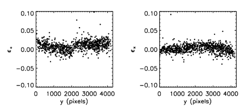
In Figure 15, we display the distribution of the mean residual ellipticity correlation for (left) and (right) after fitting TinyTim PSF to the 30 exposures in Figure 9. We used the ellipticities of all the available high S/N stars in the fields () to find the matching TinyTim PSF templates. Not surprisingly, only a small fraction of the results give reasonably small residual ellipticity correlation (). We observe that none of the 30 exposures finds the TinyTim PSF template that yields residual correlation of for both and simultaneously. Moreover, inspection of the residuals as a function of y-axis always shows a sudden, distinct discontinuity of regardless of the observation epoch. We show one such example in Figure 16, where we arbitrarily select the first exposure in Figure 9 (taken on 6 May 2002 at 1:51:21 UT).
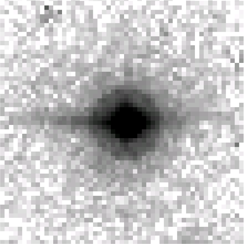
In addition to the aforementioned discrepancies between TinyTim and observed PSFs, we also point out here that the current version of TinyTim does not model a strong scatter along the CCD serial readout direction at long wavelengths (Å). This horizontal pattern (left panel of Figure 18) is caused by an anti-halation layer introduced between the CCD and its glass substrate (Sirianni et al. 1998), which is effective at suppressing a near IR halo. The feature, which contains % of the total PSF flux at , is strong in F850LP, and also visible in F814W whose transmission curve truncates at 9300 Å. The feature appears to enhance the existing horizontal diffraction spikes particularly on the left-hand side of the core. However, unlike the real diffraction spikes, this scattering feature penetrates deep into the PSF core, substantially increasing the PSF ellipticity along direction (right panel of Figure 18).
4.5 How to Select the Right PSF Template
Extracting the PSF information from stellar observations to construct a library of PSF templates is one thing, but finding a matching PSF template for a given science image is quite another. Most of the existing stellar observations in the archive are taken in short exposures (s) whereas typical science observations require integration of one or more orbits. Particularly, weak-lensing analysis of distant clusters () needs multi-orbit integration (with some dithering pattern) to achieve the aimed depth and field of view.
Therefore, we must justify that the PSF template compiled from these short exposure observations can reliably represent the PSF pattern for the long-exposure science image, which should contain the intra-orbit focus variation. Fortunately, previous studies (Jee et al. 2005a; Schrabback et al. 2007) support the fact that the short-time exposure PSF pattern can adequately serve as a mean PSF for long-exposure science observations. Rhodes et al. (2007) also claim that the TinyTim PSFs even at a fixed focus value can nicely represent the COSMOS stars except for the aforementioned pattern in the detector center.
Having accepted that the short-exposure PSFs can properly serve as average PSFs for long-exposure data, we can straightforwardly handle multi-orbit data by finding a matching PSF template for each exposure. This method is proposed by Jee et al. (2007), Schrabback et al. (2007), and Rhodes et al. (2007). Jee et al. (2007) implemented the idea of finding a matching template for each exposure from visual inspection of the star whiskers. This manual procedure soon becomes prohibitively time-consuming as the number of exposures increases. Rhodes et al. (2007) and Schrabback et al. (2007) suggested an automation of the procedure by fitting the ellipticities of the PSF model (whether derived from TinyTim or archival stellar fields) to the ellipticities of the stars in the target field. We find that this method is a workable solution in general, but can be improved by fitting the sizes of the PSFs, as well as the ellipticities. The merit is due to the observation that the sizes of the PSFs are also sensitive to the focus of . Therefore, our best fitting PSF template minimizes the following :
| (10) |
where and are the measurements of the stars in the science image and the predicted values at the same locations in the model, respectively. In the current study the uncertainties of the moments in Equation 10 were evaluated from Monte Carlo simulations; alternatively, one can use analytic approximations (e.g., Goldberg & Natarajan 2002).
We examined the reliability of the above PSF fitting by randomly drawing a small number of stars from the catalog of J8C0D1051 and fitting the template PSF from our library to these stars. The catalog of J8C0D1051 contains stars and as already shown in Figure 5 a small fraction (%) of these stars () are noisy (residual ellipticity greater than 0.02). We did not discard these noisy stars in the random selection because we want to simulate realistic cases where it is hard to judge which stars are noisy. The reliability of the PSF fitting of course depends on the properties and the locations of the selected stars. Therefore, we iterated 100 times for a given number of stars to even out the selection effect. We evaluated the quality of the fitting using the resulting ellipticity correlation functions. We consider the fitting as failure if the absolute value of the mean correlation is greater than , which is a very conservative choice (cosmic shear signals are of the order . however, they are measured from galaxies whose ellipticity correlations due to the PSF correlations are somewhat diluted). Figure 17 displays the simulation result. A few points are worthy to be discussed. First, the success rate is still high even when only 5 stars are used (7 and 13 out of 100 failures for quadrupole and ellipticity fitting, respectively). Second, the number of failure incidences for quadrupole fitting is significantly lower than for ellipticity fitting (approximately a factor of two less incidences for fewer than 15 stars). Finally, we note that even for the “failure” incidences the resulting ellipticity correlation is only moderately high ( or less).
5 CONCLUSIONS
We showed that the time- and position-dependent ACS/WFC PSF can be robustly described through PCA. The PCA technique allows us to perform orthogonal expansion of the observed PSFs with as few as 20 eigen-PSFs derived from the data themselves. This method is superior to our previous shapelet-based decomposition of the PSFs, capturing more details of the diffraction pattern of the instrument PSF. By interpolating the position-dependent variation of the eigen-PSFs with 5th order polynomials, we are able to recover the observed pattern of the PSF ellipticity and width variation. Although the TinyTim software provides a good approximation of the observed PSFs, we demonstrate that there are some important mismatches between the TinyTim prediction and the real PSFs, which cannot be attributed to CTE degradation of WFC over time. The CTE charge trailing effect should be negligible for these bright high S/N stars, and we do not observe any long-term variation of the pattern (i.e., increasing elongation in parallel read-out direction with time) due to the CTE degradation. Because typical science observations require integration of one or more orbits in broadband filters, the background levels are high ( for integration of one orbit). These high background photons are supposed to fill the charge traps and thus mitigate the CTE effects. Therefore, we argue that the CTE-induced elongation is not likely to limit the application of our PSF models extracted from short-exposure observations to long-exposure science images.
We have compiled WFC PSFs from stellar field observations, which span a wide range of focus values. Although the current paper mainly deals with the ACS/WFC PSF issue in the context of weak-lensing analysis, we believe that our PSF model can be used in a wide range of the astronomical data analyses where the knowledge of the position-dependent WFC PSF is needed (e.g., crowded field stellar photometry, robust profile fitting of small objects, weak-lensing analyses, etc.).
ACS was developed under NASA contract NAS5-32865, and this research was supported by NASA grant NAG5-7697.
References
- Anderson & King (2006) Anderson, J. & King 2006, 2006-01, Space Telescope Science Institute
- Bernstein & Jarvis (2002) Bernstein, G. M., & Jarvis, M. 2002, AJ, 123, 583
- Bromley et al. (1998) Bromley, B. C., Press, W. H., Lin, H., & Kirshner, R. P. 1998, ApJ, 505, 25
- Connolly et al. (1995) Connolly, A. J., Szalay, A. S., Bershady, M. A., Kinney, A. L., & Calzetti, D. 1995, AJ, 110, 1071
- Goldberg & Natarajan (2002) Goldberg, D. M., & Natarajan, P. 2002, ApJ, 564, 65
- Hack et al. (2003) Hack, W., Busko, I., & Jedrzejewski, R. 2003, ASP Conf. Ser. 295: Astronomical Data Analysis Software and Systems XII, 295, 453
- Hershey, J. (1997) Hershey, J. 1997, Modeling HST Focal-Length Variations V.1.1, SESD-97-01
- Heymans et al. (2005) Heymans, C., et al. 2005, MNRAS, 361, 160
- Jarvis & Jain (2004) Jarvis, M., & Jain, B. 2004, ArXiv Astrophysics e-prints, arXiv:astro-ph/0412234
- Jee et al. (2005) Jee, M. J., White, R. L., Benítez, N., Ford, H. C., Blakeslee, J. P., Rosati, P., Demarco, R., & Illingworth, G. D. 2005a, ApJ, 618, 46
- Jee et al. (2005) Jee, M. J., White, R. L., Ford, H. C., Blakeslee, J. P., Illingworth, G. D., Coe, D. A., & Tran, K.-V. H. 2005b, ApJ, 634, 813
- Jee et al. (2006) Jee, M. J., White, R. L., Ford, H. C., Illingworth, G. D., Blakeslee, J. P., Holden, B., & Mei, S. 2006, ApJ, 642, 720
- Jee et al. (2007) Jee, M. J., Ford, H. C., Illingworth, G. D., , White, R. L., Broadhurst, T. J., Coe, D. A., Meurer, G. R., van der Wel, A., Benitez, N., Blakeslee, J. P., Bouwens, R. J., Bradley, L., Demarco, R., Homeier, N. L. , Martel, A. R., & & Mei, S. 2007, ApJ, 661, 728
- Krist (2003) Krist, J. 2003, 2003-06, Space Telescope Science Institute
- Lauer (2002) Lauer, T. R. 2002, ArXiv Astrophysics e-prints, arXiv:astro-ph/0208247
- Lupton et al. (2001) Lupton, R., Gunn, J. E., Ivezić, Z., Knapp, G. R., & Kent, S. 2001, Astronomical Data Analysis Software and Systems X, 238, 269
- Madgwick et al. (2003) Madgwick, D. S., et al. 2003, ApJ, 599, 997
- Press et al. (1992) Press, W.H., Teukolsky, S.A., Vetterling, W.T., Flannery, B.P. 1992, Numerical Recipes. Cambridge (Cambridge University Press)
- Refregier (2003) Refregier, A. 2003, MNRAS, 338, 35
- Rhodes et al. (2007) Rhodes, J. D., et al. 2007, ArXiv Astrophysics e-prints, arXiv:astro-ph/0702140
- Riess and Mack (2004) Riess, A. & Mack, J. 2004, 2004-006, Space Telescope Science
- Schrabback et al. (2007) Schrabback, T., et al. 2007, A&A, 468, 823
- Sirianni et al. (1998) Sirianni, M., et al. 1998, Proc. SPIE, 3355, 608


