Three-body equations of motion in successive post-Newtonian approximations

Carlos O. Lousto and Hiroyuki Nakano Center for Computational Relativity and Gravitation, School of Mathematical Sciences,
Rochester Institute of Technology, Rochester, New York 14623, USA
Abstract

There are periodic solutions to the equal-mass three-body (and N𝑁N-body) problem in Newtonian gravity. The figure-eight solution is one of them. In this paper, we discuss its solution in the first and second post-Newtonian approximations to General Relativity. To do so we derive the canonical equations of motion in the ADM gauge from the three-body Hamiltonian. We then integrate those equations numerically, showing that quantities such as the energy, linear and angular momenta are conserved down to numerical error. We also study the scaling of the initial parameters with the physical size of the triple system. In this way we can assess when general relativistic results are important and we determine that this occur for distances of the order of 100M100𝑀100M, with M𝑀M the total mass of the system. For distances much closer than those, presumably the system would completely collapse due to gravitational radiation. This sets up a natural cut-off to Newtonian N𝑁N-body simulations. The method can also be used to dynamically provide initial parameters for subsequent full nonlinear numerical simulations.

pacs:
95.10.Ce, 95.30.Sf, 45.50.Pk, 04.25.Nx

I Introduction

The closest star to the solar system, Alpha Centauri, is a triple system, so is Polaris and HD 188753. Triple stars and black holes are common in globular clusters Gultekin et al. (2003); Miller and Hamilton (2002), and galactic disks. Triple black hole mergers can be formed in galaxy merger Valtonen (1996) and a triple quasar, representing a triple supermassive black hole system has been recently discovered Djorgovski et al. (2007).

Full numerical simulations of black holes made possible only in the last couple of years have already produced numerous astrophysically interesting results, among them, the orbital hangup and respect of the cosmic censorship hypothesis for spinning black holes Campanelli et al. (2006a, b, 2007a), precession and spin-flips Campanelli et al. (2007a), and the discovery Campanelli et al. (2007b) of large recoil velocities in highly-spinning black hole mergers up to 4,00040004,000 km/s Campanelli et al. (2007c).

The 2005 breakthroughs in Numerical Relativity Pretorius (2005); Campanelli et al. (2006c); Baker et al. (2006), not only provided a solution to the long standing two-body problem in General Relativity, but it also proved applicable to the black hole - neutron star binaries Faber et al. (2007) and recently to the three (and N𝑁N) - black holes systems Campanelli et al. (2007d).

In general, the solution of three-body problem in Newtonian gravity can be chaotic. There are however, periodic orbits in the problem of three equal masses on a plane. One of the most surprising solution is a figure-eight orbit. The three bodies chase each other forever around a fixed eight-shaped curve. This was found first by Moore Moore (1993) and discussed with the proof of the existence in Ref. Chenciner and Montgomery (2000). Heggie Heggie (2000) also estimates the probability for such systems to occur in a galaxy.

Because of effects such as the perihelion shift, it was unclear if the figure-eight orbits would exist in a low post-Newtonian expansion, even if it consist of only conservative terms. Imai, Chiba and Asada succeeded in obtaining the figure-eight solution in a first post-Newtonian order approximation by finding the general relativistic corrections to the Newtonian initial conditions. In Ref. Chiba et al. (2007) they also estimated the periodic gravitational waves from this system.

In Ref. Imai et al. (2007) was used the Euler-Lagrange equations of motion in an approximation to first post-Newtonian order. In our paper we instead assume the Hamiltonian formulation to derive the equations of motion. We start from the Hamiltonian given in Ref. Schäfer (1987) (with typos corrected in our Appendix). We derive the equations of motion in this formalism, which are different from those used in Ref. Imai et al. (2007) and have the virtue of explicitly satisfying the constants of motion of the problem, and thus being more amenable to numerical integration.

The paper is organized as follows. In Section II, we summarize the equations of motion to be solved numerically in order to obtain the figure-eight orbits. The starting point is the three-body Hamiltonian in the first post-Newtonian approximation. In Section III, we discuss the initial conditions for the figure-eight solutions. We study the scaling relation between the orbital radius and the linear momenta. From this analysis, we can estimate when general relativistic effects are important. In Section IV, we extend our calculation to the second post-Newtonian order and in Section V, we summarize the results of this paper and discuss some remaining problems. The 2PN three-body Hamiltonian is explicitly given in the Appendix. Throughout this paper, we use units in which c=G=1𝑐𝐺1c=G=1.

II Equations of motion

As we mentioned in the introduction, the Newtonian configuration that leads to orbital braid figures can also be obtained within the Lagrangian approach, in the first post-Newtonian approximation, by finding the appropriate corrections to the initial data Imai et al. (2007).

Here we will consider the Hamiltonian formulation since it generates equations of motion that conserve the energy, linear and angular momenta. This is crucial to reach high accuracy in the numerical integrations, which is needed to keep good track of the orbital motion, that in the three body problem might be chaotic.

The Hamiltonian (H=HN+H1PN+H2PN𝐻subscript𝐻𝑁subscript𝐻1𝑃𝑁subscript𝐻2𝑃𝑁H=H_{N}+H_{1PN}+H_{2PN}) for the three body problem in the second post-Newtonian approximation is given next. Note that since gravitational radiation only enters at 2.5PN2.5𝑃𝑁2.5PN-order and higher, the current analysis applies to conservative systems.

The Newtonian Hamiltonian is given by

HNsubscript𝐻𝑁\displaystyle H_{N} =\displaystyle= 12apa2ma12a,bamambrab,12subscript𝑎superscriptsubscript𝑝𝑎2subscript𝑚𝑎12subscript𝑎𝑏𝑎subscript𝑚𝑎subscript𝑚𝑏subscript𝑟𝑎𝑏\displaystyle\frac{1}{2}\sum_{a}\frac{p_{a}^{2}}{m_{a}}-\frac{1}{2}\sum_{a,b\neq a}\frac{m_{a}m_{b}}{r_{ab}}\,, (1)

and to the first post-Newtonian order by

H1PNsubscript𝐻1𝑃𝑁\displaystyle H_{1PN} =\displaystyle= 18ama(pa2ma2)218subscript𝑎subscript𝑚𝑎superscriptsuperscriptsubscript𝑝𝑎2superscriptsubscript𝑚𝑎22\displaystyle-\frac{1}{8}\sum_{a}m_{a}\left(\frac{p_{a}^{2}}{m_{a}^{2}}\right)^{2} (2)
14a,bamambrab{6pa2ma27𝐩a𝐩bmamb\displaystyle-\frac{1}{4}\sum_{a,b\neq a}\frac{m_{a}m_{b}}{r_{ab}}\Big{\{}6\frac{p_{a}^{2}}{m_{a}^{2}}-7\frac{{\bf p}_{a}\cdot{\bf p}_{b}}{m_{a}m_{b}}
(𝐧ab𝐩a)(𝐧ab𝐩b)mamb}\displaystyle-\frac{\left({\bf n}_{ab}\cdot{\bf p}_{a}\right)\left({\bf n}_{ab}\cdot{\bf p}_{b}\right)}{m_{a}m_{b}}\Big{\}}
+12a,ba,camambmcrabrac,12subscriptformulae-sequence𝑎𝑏𝑎𝑐𝑎subscript𝑚𝑎subscript𝑚𝑏subscript𝑚𝑐subscript𝑟𝑎𝑏subscript𝑟𝑎𝑐\displaystyle+\frac{1}{2}\sum_{a,b\neq a,c\neq a}\frac{m_{a}m_{b}m_{c}}{r_{ab}r_{ac}}\,,

where a,b𝑎𝑏a,\,b and c𝑐c run over 1, 2121,\,2 and 333. We have used the notations; 𝐱ab=𝐱a𝐱bsubscript𝐱𝑎𝑏subscript𝐱𝑎subscript𝐱𝑏{\bf x}_{ab}={\bf x}_{a}-{\bf x}_{b}, rab=|𝐱ab|subscript𝑟𝑎𝑏subscript𝐱𝑎𝑏r_{ab}=|{\bf x}_{ab}|, 𝐧ab=𝐱ab/rabsubscript𝐧𝑎𝑏subscript𝐱𝑎𝑏subscript𝑟𝑎𝑏{\bf n}_{ab}={\bf x}_{ab}/r_{ab}, pa2=𝐩a𝐩asuperscriptsubscript𝑝𝑎2subscript𝐩𝑎subscript𝐩𝑎p_{a}^{2}={\bf p}_{a}\cdot{\bf p}_{a} and the dot (\cdot) means the inner product. The Hamiltonian for the second post-Newtonian order is given in the Appendix.

We then obtain the canonical equations

(p˙a)i=H(qa)i,(q˙a)i=H(pa)i,formulae-sequencesubscriptsubscript˙𝑝𝑎𝑖𝐻subscriptsubscript𝑞𝑎𝑖subscriptsubscript˙𝑞𝑎𝑖𝐻subscriptsubscript𝑝𝑎𝑖\displaystyle({\dot{p}}_{a})_{i}=-\frac{\partial H}{\partial(q_{a})_{i}}\,,\qquad({\dot{q}}_{a})_{i}=\frac{\partial H}{\partial(p_{a})_{i}}\,, (3)

where i𝑖i denotes x,y𝑥𝑦x,\,y or z𝑧z.

Explicitly, the equation of motion for the first post-Newtonian order, are given for the particle 1 by

t𝐱𝟏𝑡subscript𝐱1\displaystyle{\frac{\partial}{\partial t}}\,{\bf{x}_{1}} =\displaystyle= 𝐩1m112(𝐩1𝐩1)𝐩1m13subscript𝐩1subscript𝑚112subscript𝐩1subscript𝐩1subscript𝐩1superscriptsubscript𝑚13\displaystyle{\displaystyle\frac{{{\bf p}_{1}}}{{m_{1}}}}-{\displaystyle\frac{1}{2}}\,{\displaystyle\frac{\,({{\bf p}_{1}}\cdot{{\bf p}_{1}})\,{{\bf p}_{1}}}{{m_{1}}^{3}}} (4)
12m1m2r12(6𝐩1m1272𝐩2m1m2\displaystyle-{\displaystyle\frac{1}{2}}\,{\displaystyle\frac{{m_{1}}\,{m_{2}}}{{r_{12}}}}\,\left(\!{\displaystyle\frac{6\,{{\bf p}_{1}}}{{m_{1}}^{2}}}-{\displaystyle\frac{7}{2}}\,{\displaystyle\frac{{{\bf p}_{2}}}{{m_{1}}\,{m_{2}}}}\right.
12(𝐩2𝐱12)𝐱12m1m2r122)\displaystyle\left.-{\displaystyle\frac{1}{2}}\,{\displaystyle\frac{\,({{\bf p}_{2}}\cdot{{\bf x}_{12}}){{\bf x}_{12}}}{{m_{1}}\,{m_{2}}\,{r_{12}}^{2}}}\!\right)
+12(72𝐩3r31+12(𝐩3𝐱31)𝐱31r313)1272subscript𝐩3subscript𝑟3112subscript𝐩3subscript𝐱31subscript𝐱31superscriptsubscript𝑟313\displaystyle+{\displaystyle\frac{1}{2}}\,\left(\!{\displaystyle\frac{7}{2}}\,{\displaystyle\frac{{{\bf p}_{3}}}{{r_{31}}}}+{\displaystyle\frac{1}{2}}\,{\displaystyle\frac{({{\bf p}_{3}}\cdot{{\bf x}_{31}})\,{{\bf x}_{31}}}{{r_{31}}^{3}}}\!\right)
12m1m3r31(6𝐩1m1272𝐩3m1m3\displaystyle-{\displaystyle\frac{1}{2}}\,{\displaystyle\frac{{m_{1}}\,{m_{3}}}{{r_{31}}}}\,\left(\!{\displaystyle\frac{6\,{{\bf p}_{1}}}{{m_{1}}^{2}}}-{\displaystyle\frac{7}{2}}\,{\displaystyle\frac{{{\bf p}_{3}}}{{m_{1}}\,{m_{3}}}}\right.
12(𝐩3𝐱31)𝐱31m3m1r312)\displaystyle\left.-{\displaystyle\frac{1}{2}}\,{\displaystyle\frac{({{\bf p}_{3}}\cdot{{\bf x}_{31}})\,{{\bf x}_{31}}}{{m_{3}}\,{m_{1}}\,{r_{31}}^{2}}}\!\right)
+12(72𝐩2r12+12(𝐩2𝐱12)𝐱12r123),1272subscript𝐩2subscript𝑟1212subscript𝐩2subscript𝐱12subscript𝐱12superscriptsubscript𝑟123\displaystyle+{\displaystyle\frac{1}{2}}\,\left(\!{\displaystyle\frac{7}{2}}\,{\displaystyle\frac{{{\bf p}_{2}}}{{r_{12}}}}+{\displaystyle\frac{1}{2}}\,{\displaystyle\frac{({{\bf p}_{2}}\cdot{{\bf x}_{12}})\,{{\bf x}_{12}}}{{r_{12}}^{3}}}\!\right)\,,
t𝐩1𝑡subscript𝐩1\displaystyle{\frac{\partial}{\partial t}}\,{{\bf p}_{1}} =\displaystyle= 𝐱12r12(m1m2r122m2m1m3r122r2, 3m1m2m3r122r31\displaystyle-\frac{{\bf x}_{12}}{{r_{12}}}\left({\vrule height=13.09999pt,width=0.0pt,depth=13.09999pt}\right.\!\!{\displaystyle\frac{{m_{1}}\,{m_{2}}}{{r_{12}}^{2}}}-{\displaystyle\frac{{m_{2}}\,{m_{1}}\,{m_{3}}}{{r_{12}}^{2}\,{r_{2,\,3}}}}-{\displaystyle\frac{{m_{1}}\,{m_{2}}\,{m_{3}}}{{r_{12}}^{2}\,{r_{31}}}} (5)
+12m1m2r122(3(𝐩1𝐩1)m12+3(𝐩2𝐩2)m22\displaystyle+{\displaystyle\frac{1}{2}}{\displaystyle\frac{{m_{1}}\,{m_{2}}}{{r_{12}}^{2}}}\left({\vrule height=13.09999pt,width=0.0pt,depth=13.09999pt}\right.\!\!{\displaystyle\frac{3\,({{\bf p}_{1}}\cdot{{\bf p}_{1}})}{{m_{1}}^{2}}}+{\displaystyle\frac{3\,({{\bf p}_{2}}\cdot{{\bf p}_{2}})}{{m_{2}}^{2}}}
7(𝐩1𝐩2)m1m2(𝐩1𝐱12)(𝐩2𝐱12)m1m2r122)\displaystyle-{\displaystyle\frac{7\,({{\bf p}_{1}}\cdot{{\bf p}_{2}})}{{m_{1}}\,{m_{2}}}}-{\displaystyle\frac{({{\bf p}_{1}}\cdot{{\bf x}_{12}})\,({{\bf p}_{2}}\cdot{{\bf x}_{12}})}{{m_{1}}\,{m_{2}}\,{r_{12}}^{2}}}\!\!\left.{\vrule height=13.09999pt,width=0.0pt,depth=13.09999pt}\right)
(𝐩1𝐱12)(𝐩2𝐱12)r124m2m12r123m1m22r123)\displaystyle-{\displaystyle\frac{({{\bf p}_{1}}\cdot{{\bf x}_{12}})\,({{\bf p}_{2}}\cdot{{\bf x}_{12}})}{{r_{12}}^{4}}}-{\displaystyle\frac{{m_{2}}\,{m_{1}}^{2}}{{r_{12}}^{3}}}-{\displaystyle\frac{\,{m_{1}}\,{m_{2}}^{2}}{{r_{12}}^{3}}}\!\!\left.{\vrule height=13.09999pt,width=0.0pt,depth=13.09999pt}\right)
+𝐱31r31(m3m1r312m3m1m2r312r2, 3m1m2m3r12r312\displaystyle+\frac{{\bf x}_{31}}{{r_{31}}}\left({\vrule height=13.09999pt,width=0.0pt,depth=13.09999pt}\right.\!\!{\displaystyle\frac{{m_{3}}\,{m_{1}}}{{r_{31}}^{2}}}-{\displaystyle\frac{{m_{3}}\,{m_{1}}\,{m_{2}}}{{r_{31}}^{2}\,{r_{2,\,3}}}}-{\displaystyle\frac{{m_{1}}\,{m_{2}}\,{m_{3}}}{{r_{12}}\,{r_{31}}^{2}}}
+12m3m1r312(3(𝐩3𝐩3)m32+3(𝐩1𝐩1)m12\displaystyle+{\displaystyle\frac{1}{2}}{\displaystyle\frac{{m_{3}}\,{m_{1}}}{{r_{31}}^{2}}}\left({\vrule height=13.09999pt,width=0.0pt,depth=13.09999pt}\right.\!\!{\displaystyle\frac{3\,({{\bf p}_{3}}\cdot{{\bf p}_{3}})}{{m_{3}}^{2}}}+{\displaystyle\frac{3\,({{\bf p}_{1}}\cdot{{\bf p}_{1}})}{{m_{1}}^{2}}}
7(𝐩1𝐩3)m1m3(𝐩3𝐱31)(𝐩1𝐱31)m3m1r312)\displaystyle-{\displaystyle\frac{7\,({{\bf p}_{1}}\cdot{{\bf p}_{3}})}{{m_{1}}\,{m_{3}}}}-{\displaystyle\frac{({{\bf p}_{3}}\cdot{{\bf x}_{31}})\,({{\bf p}_{1}}\cdot{{\bf x}_{31}})}{{m_{3}}\,{m_{1}}\,{r_{31}}^{2}}}\!\!\left.{\vrule height=13.09999pt,width=0.0pt,depth=13.09999pt}\right)
(𝐩3𝐱31)(𝐩1𝐱31)r314m3m12r313m1m32r313)\displaystyle-{\displaystyle\frac{{({\bf p}_{3}}\cdot{{\bf x}_{31}})\,({{\bf p}_{1}}\cdot{{\bf x}_{31}})}{{r_{31}}^{4}}}-{\displaystyle\frac{{m_{3}}\,{m_{1}}^{2}}{{r_{31}}^{3}}}-{\displaystyle\frac{{m_{1}}\,{m_{3}}^{2}}{{r_{31}}^{3}}}\!\!\left.{\vrule height=13.09999pt,width=0.0pt,depth=13.09999pt}\right)
12((𝐩2𝐱12)𝐩1r123+(𝐩1𝐱12)𝐩2r123)12subscript𝐩2subscript𝐱12subscript𝐩1superscriptsubscript𝑟123subscript𝐩1subscript𝐱12subscript𝐩2superscriptsubscript𝑟123\displaystyle-{\displaystyle\frac{1}{2}}\,\left(\!{\displaystyle\frac{({{\bf p}_{2}}\cdot{{\bf x}_{12}})\,{{\bf p}_{1}}}{{r_{12}}^{3}}}+{\displaystyle\frac{({{\bf p}_{1}}\cdot{{\bf x}_{12}})\,{{\bf p}_{2}}}{{r_{12}}^{3}}}\!\right)
+12((𝐩1𝐱31)𝐩3r313+(𝐩3𝐱31)𝐩1r313),12subscript𝐩1subscript𝐱31subscript𝐩3superscriptsubscript𝑟313subscript𝐩3subscript𝐱31subscript𝐩1superscriptsubscript𝑟313\displaystyle+{\displaystyle\frac{1}{2}}\,\left(\!{\displaystyle\frac{({{\bf p}_{1}}\cdot{{\bf x}_{31}})\,{{\bf p}_{3}}}{{r_{31}}^{3}}}+{\displaystyle\frac{({{\bf p}_{3}}\cdot{{\bf x}_{31}})\,{{\bf p}_{1}}}{{r_{31}}^{3}}}\!\right)\,,

where to obtain the equation of motion for the particle 2 (and 3), we change the subscripts as {12,23,31}formulae-sequence12formulae-sequence2331\{1\to 2,2\to 3,3\to 1\} (and {13,21,32}formulae-sequence13formulae-sequence2132\{1\to 3,2\to 1,3\to 2\}), respectively.

We solved the above equations numerically for three body problems using a 10 digits precision implemented in Maple 10 with typical runs of a few seconds on a Laptop. Since we use the canonical momentum in the calculation, the Hamiltonian H𝐻H, the total linear momentum 𝐏=𝐩a𝐏subscript𝐩𝑎{\bf P}=\sum{\bf p}_{a} and angular momentum 𝐋=𝐱a×𝐩a𝐋subscript𝐱𝑎subscript𝐩𝑎{\bf L}=\sum{\bf x}_{a}\times{\bf p}_{a} are conserved quantities. These represent useful checks of the accuracy of the numerical runs.

III The first post-Newtonian corrections

In the Newtonian case, a figure-eight motion can be obtained from the following initial conditions Imai et al. (2007), i.e., the positions 𝐥𝐥{\bf l} and linear momenta 𝐩𝐩{\bf p}:

𝐥𝐥\displaystyle{\bf l} =\displaystyle= (x1,y1)=(x2,y2)subscript𝑥1subscript𝑦1subscript𝑥2subscript𝑦2\displaystyle(x_{1},\,y_{1})=(-x_{2},\,-y_{2})
=\displaystyle= (97.00,24.31),97.0024.31\displaystyle(97.00,\,-24.31)\,,
(x3,y3)subscript𝑥3subscript𝑦3\displaystyle(x_{3},\,y_{3}) =\displaystyle= (0, 0),0 0\displaystyle(0,\,0)\,,
𝐩Nsubscript𝐩𝑁\displaystyle{\bf p}_{N} =\displaystyle= (p3x,p3y)=(2p1x,2p1y)=(2p2x,2p2y)superscriptsubscript𝑝3𝑥superscriptsubscript𝑝3𝑦2superscriptsubscript𝑝1𝑥2superscriptsubscript𝑝1𝑦2superscriptsubscript𝑝2𝑥2superscriptsubscript𝑝2𝑦\displaystyle(p_{3}^{x},\,p_{3}^{y})=(-2p_{1}^{x},\,-2p_{1}^{y})=(-2p_{2}^{x},\,-2p_{2}^{y}) (6)
=\displaystyle= (0.09324,0.08647).0.093240.08647\displaystyle(-0.09324,\,-0.08647)\,.

Here, we set m1=m2=m3=m=1subscript𝑚1subscript𝑚2subscript𝑚3𝑚1m_{1}=m_{2}=m_{3}=m=1. For the above initial condition, the total linear momentum and angular momentum are zero.

At the 1PN order, we also impose the total linear momentum 𝐏=0𝐏0{\bf P}=0 and the total angular momentum 𝐋=0𝐋0{\bf L}=0. By these conditions, we find that each linear momentum is given by the relations

𝐩3=2𝐩1=2𝐩2.subscript𝐩32subscript𝐩12subscript𝐩2\displaystyle{\bf p}_{3}=-2{\bf p}_{1}=-2{\bf p}_{2}\,. (7)

Therefore, when we give the positions of the three particles, and it is necessary then only to search numerically for 𝐩3subscript𝐩3{\bf p}_{3}. In order to obtain, 𝐩3subscript𝐩3{\bf p}_{3}, we make some iterative computations until the figure-eight is reproduced for a few orbits.

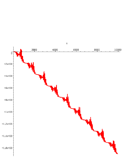
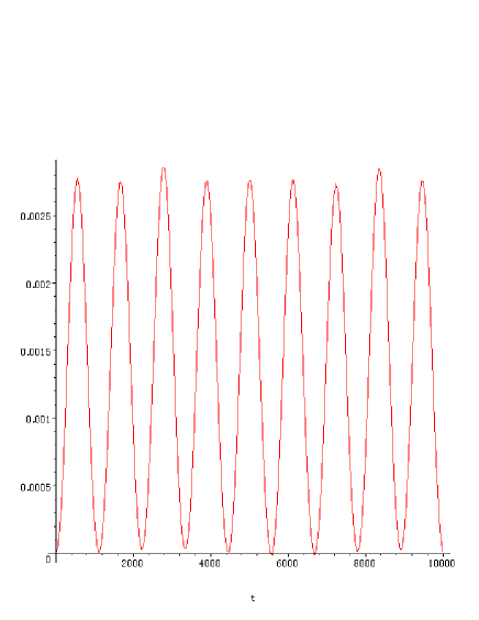
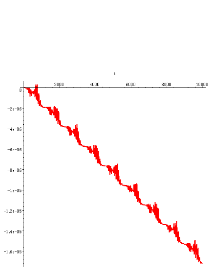
In Figures 1 and 2 we show the relative error of the Hamiltonian conservation:

ΔH(t)=H(t)H(0)H(0).Δ𝐻𝑡𝐻𝑡𝐻0𝐻0\displaystyle\Delta H(t)=\frac{H(t)-H(0)}{H(0)}\,.

Figure 1 is estimated by using the orbit calculated in Imai et al. (2007) and we observe that they lead to violations of the order of 3×1033superscript1033\times 10^{-3}. While, Figure 2 is derived by using the canonical equations derived in our paper and they display errors of the order of 106superscript10610^{-6}, growing linearly in time due to the propagation of numerical errors triggered by initial roundoff.
Refer to caption
Figure 1: The relative error of the Hamiltonian constraint in the Lagrangian approximation. This figure is derived by using the orbit in Imai et al. (2007).
Refer to caption
Figure 2: The relative error of the Hamiltonian constraint evaluate by using the orbit derived from the Hamiltonian formalism.

Next we will discuss the scaling behavior of 𝐩𝟑subscript𝐩3{\bf p_{3}} when we change the initial separation as 𝐥λ𝐥𝐥𝜆𝐥{\bf l}\to\lambda{\bf l}, and hence the size of the orbit. Note that 𝐩𝟑λ1/2𝐩𝟑subscript𝐩3superscript𝜆12subscript𝐩3{\bf p_{3}}\to\lambda^{-1/2}{\bf p_{3}} in the Newtonian limit as can be easily derived from the Hamiltonian in Eq. (1) or the equations of motion (4).

In Table 1, we summarize our numerical findings for the 1PN1𝑃𝑁1PN initial conditions for λ𝜆\lambda from 1 to 100. We note that 𝐩3subscript𝐩3{\bf p}_{3} with λ=1𝜆1\lambda=1 is different from the value which are derived from the initial velocity of Imai et al. (2007). The value θ𝜃\theta in the table is the inclination angle of the principal axes. The principal axes of the 1PN figure-eight motion are not along the x and y axes Imai et al. (2007).

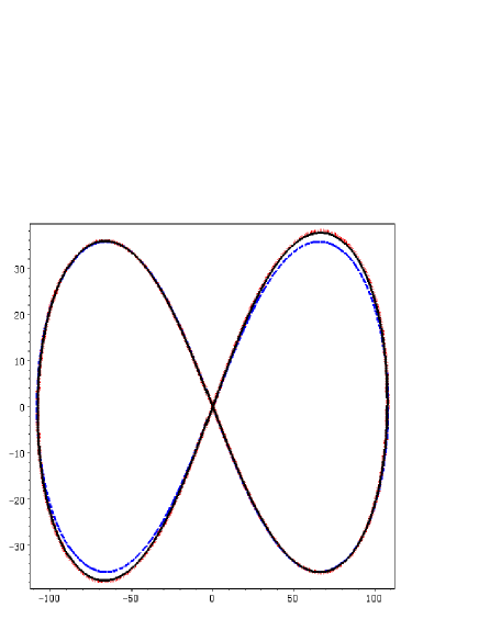
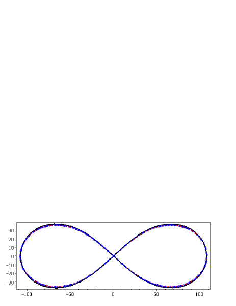
In Figure 3, the figure-eight rescaled orbits with λ=1, 10𝜆110\lambda=1,\,10 and 100100100 are shown. Here, in order to display the general relativistic effects, we have used the coordinates: (xa(t)/λ,ya(t)/λ)subscript𝑥𝑎𝑡𝜆subscript𝑦𝑎𝑡𝜆(x_{a}(t)/\lambda,\,y_{a}(t)/\lambda). We have chosen here the x-axis as the principal axis. We observe that the superposition of the λ=10𝜆10\lambda=10 and λ=100𝜆100\lambda=100 is suggestive that at those scales the general relativistic effects are very small while for λ<1𝜆1\lambda<1 they are dominant, but remainder gauge effects may also mask this effect because the orbits are not gauge invariant. A cleaner analysis can be made directly looking at the initial linear momenta scaling.

Table 1: The initial conditions and inclination angle.
λ𝜆\lambda (p3)xsubscriptsubscript𝑝3𝑥(p_{3})_{x} (p3)ysubscriptsubscript𝑝3𝑦(p_{3})_{y} θ𝜃\theta
1.00 -0.09811067089 -0.09490870640 0.01535863098
2.00 -0.06754964265 -0.06392246619 0.007238984240
5.00 -0.04209168100 -0.03934705365 0.002786451510
10.00 -0.02961805051 -0.02758150399 0.001351084509
20.00 -0.02089989478 -0.01941808121 0.0006871250545
50.00 -0.01319661317 -0.01225031026 0.0002447024114
100.00 -0.009328662000 -0.008654573162 0.0001269692928

By using the results of the runs in Table 1, we propose a fitting formula for |𝐩3|subscript𝐩3|{\bf p}_{3}| inspired again in the 1PN Hamiltonian or the equations of motion

|𝐩3|fit(λ)=0.01617387234λ+0.002042558971λ2+0.0004169461512λ3.subscriptsubscript𝐩3fit𝜆0.01617387234𝜆0.002042558971superscript𝜆20.0004169461512superscript𝜆3\displaystyle|{\bf p}_{3}|_{\rm fit}(\lambda)=\sqrt{\frac{0.01617387234}{\lambda}+\frac{0.002042558971}{\lambda^{2}}+\frac{0.0004169461512}{\lambda^{3}}}\,. (8)

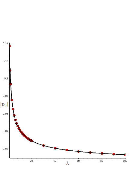
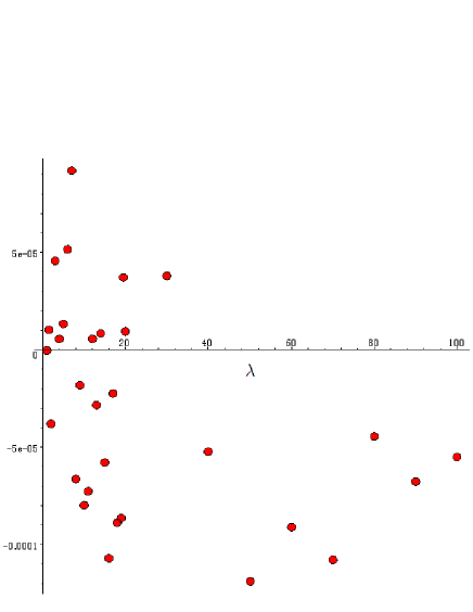
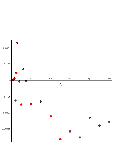
In Figure 4, we show the fitting function and in Figure 5 we display the relative error |𝐩3||𝐩3|fit/|𝐩3|subscript𝐩3subscriptsubscript𝐩3fitsubscript𝐩3|{\bf p}_{3}|-|{\bf p}_{3}|_{\rm fit}/|{\bf p}_{3}|  , consistent with the form of an error generated in the numerical calculation.
Refer to caption
Figure 3: Figure-eight motions. We show λ=1𝜆1\lambda=1 (solid line) λ=10𝜆10\lambda=10 (dashed line) and λ=100𝜆100\lambda=100 (dotted line).
Refer to caption
Figure 4: λ𝜆\lambda-|𝐩3|subscript𝐩3|{\bf p}_{3}| relation with points obtained numerically.
Refer to caption
Figure 5: The relative error of the fitting.

Independently in the Newtonian calculations, the λ𝜆\lambda-|𝐩3|subscript𝐩3|{\bf p}_{3}| relation can be obtained from the initial condition in Eqs. (6) as

|𝐩3|N(λ)=0.1271642973λ1/2.subscriptsubscript𝐩3N𝜆0.1271642973superscript𝜆12\displaystyle|{\bf p}_{3}|_{\rm N}(\lambda)=\frac{0.1271642973}{\lambda^{1/2}}\,. (9)

Note that relative difference |𝐩3|subscript𝐩3|{\bf p}_{3}| between the Newtonian and the first post-Newtonian calculations:

|𝐩3|fit(λ)|𝐩3|N(λ)|𝐩3|N(λ),subscriptsubscript𝐩3fit𝜆subscriptsubscript𝐩3N𝜆subscriptsubscript𝐩3N𝜆\displaystyle\frac{|{\bf p}_{3}|_{\rm fit}(\lambda)-|{\bf p}_{3}|_{\rm N}(\lambda)}{|{\bf p}_{3}|_{\rm N}(\lambda)}\,,

is 7% for λ=1𝜆1\lambda=1, 0.6% for λ=10𝜆10\lambda=10 and 0.07% for λ=100𝜆100\lambda=100.

IV Second post-Newtonian corrections

It is interesting to verify if this kind of orbits also exists in the second post-Newtonian approximation to General Relativity, since they incorporate further effects of the curvature, but yet not gravitational radiation. The calculations are done by using the same method as for the first post-Newtonian order. In Table 2, we summarize the initial conditions for each λ𝜆\lambda from 1 to 100. We show the numerical errors as measured through the Hamiltonian non-conservation in Figure 6.

We find that we can approximate |𝐩3|subscript𝐩3|{\bf p}_{3}| by the fitting formula

|𝐩3|fit(λ)=0.01617654493λ+0.002017242451λ2+0.0002017242451λ3+0.0001054698539λ4.subscriptsubscript𝐩3fit𝜆0.01617654493𝜆0.002017242451superscript𝜆20.0002017242451superscript𝜆30.0001054698539superscript𝜆4\displaystyle|{\bf p}_{3}|_{\rm fit}(\lambda)=\sqrt{\frac{0.01617654493}{\lambda}+\frac{0.002017242451}{\lambda^{2}}+\frac{0.0002017242451}{\lambda^{3}}+\frac{0.0001054698539}{\lambda^{4}}}\,. (10)

There is a significant difference between the coefficient of 1/λ31superscript𝜆31/\lambda^{3} in Eqs. (8) and (10). This is due to second post-Newtonian corrections entering in this coefficient, as we can verify from the form of the Hamiltonian.

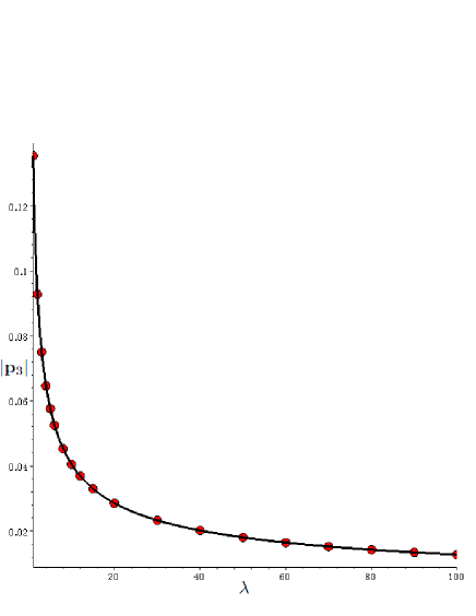
In Figure 7, we show the fitting function while its relative error is given in Figure 8.

Table 2: The initial conditions and inclination angle for the second post-Newtonian case.
λ𝜆\lambda (p3)xsubscriptsubscript𝑝3𝑥(p_{3})_{x} (p3)ysubscriptsubscript𝑝3𝑦(p_{3})_{y} θ𝜃\theta
1.00 -0.09759146109 -0.09386471063 0.01335212441
2.00 -0.06746813797 -0.06375625776 0.006775950067
5.00 -0.04208326266 -0.03933131483 0.002713363325
10.00 -0.02961805051 -0.02757874584 0.001340868765
20.00 -0.02089780479 -0.01941808121 0.0006733410290
50.00 -0.01319661317 -0.01225031026 0.0002447024114
100.00 -0.009328662000 -0.008654573162 0.0001269692928
Refer to caption
Figure 6: The relative error of the Hamiltonian conservation for the second post-Newtonian order calculations.
Refer to caption
Figure 7: λ𝜆\lambda-|𝐩3|subscript𝐩3|{\bf p}_{3}| relation for the second post-Newtonian case. The points are obtained numerically.
Refer to caption
Figure 8: The relative fitting error for the second post-Newtonian case.

Finally, we summarize the results by showing the difference between the Newtonian, first and second post-Newtonian results in Figure 9. The second post-Newtonian effect is small but clearly not negligible for λ=1𝜆1\lambda=1.

Refer to caption
Figure 9: Comparison of figure-eight motions for λ=1𝜆1\lambda=1. The solid, dotted and dashed lines show the 2PN, 1PN and Newtonian results, respectively.

V Discussion

In this paper we have used the figure-eight orbits as a theoretical lab to test the properties of the low post-Newtonian expansions of General Relativity. We have found that those closed orbits exists for three (and presumably N𝑁N) bodies. We have provided an improved first-post-Newtonian order formalism for deriving the equations of motion that satisfy the Hamiltonian (the linear and angular momenta) constraint to round-off error. The subsequent numerical evolution is well behaved during for more than t10,000msimilar-to𝑡10000𝑚t\sim 10,000m. We have also extended this analysis to the 2PN2𝑃𝑁2PN corrections, still giving a conservative system of equations. In the process of finding the figure-eight solutions by trial of different initial momenta we also showed (numerically) the stability of the orbit against small perturbations.

This method is particularly useful to determine, dynamically (as an alternative to determine them through families of initial data Campanelli et al. (2006d)), initial orbital parameters for subsequent full numerical evolution Campanelli et al. (2007d), when the holes are close enough that general relativistic effects can no longer be ignored. Note that our method fully takes into account the three-body post-Newtonian interactions unlike other simulations that approximate the problem in successive two-body problems Aarseth (2007).

It is interesting to note here that the scaling fits (10) give a practical way to determine when relativistic or Newtonian approaches are appropriate. For λ=1𝜆1\lambda=1 we have that the ratio of the first coefficient, 0.016176544930.016176544930.01617654493 (Newtonian) to the second coefficient 0.0020172424510.0020172424510.002017242451 first-post-Newtonian is nearly 0.12/λ0.12𝜆0.12/\lambda and the second coefficient to the third one 0.00024636052270.00024636052270.0002463605227 (dominated by second-post-Newtonian) is also approximately 0.12/λ0.12𝜆0.12/\lambda. This indicates that post-Newtonian corrections are important. For λ=1𝜆1\lambda=1 the distance between the initial bodies is 200m200𝑚200m, what indicates that for nearly 67M67𝑀67M with M3m𝑀3𝑚M\approx 3m the total mass of the system has strong post-Newtonian effects. For λ1much-greater-than𝜆1\lambda\gg 1 Newtonian gravity should describe the system accurately, while for λ<1𝜆1\lambda<1 general relativistic effects should be very important, eventually leading to the total collapse of the system. It is interesting to remark here that most of the N𝑁N-body codes use some sort of regularization of the Newtonian gravity for very close encounters Aarseth (2003), instead the natural way to regularize these close encounters Campanelli et al. (2007d) is given by the General Theory of Relativity, and as we show here, the post-Newtonian corrections are already non-negligible at separations of the order of 100M100𝑀100M. In any case, for most of the astrophysical encounters this is way too short distance, but it can obviously be reached in systems involving black holes and neutron stars.

Acknowledgements.
We would like to thank H.-P. Bischof, M. Campanelli, A. Gualandris, D. Merritt, D. Ross and Y. Zlochower for useful discussions. This is supported by JSPS for Research Abroad (HN) and by the NSF through grants PHY-0722315, PHY-0701566, PHY-0714388, and PHY-0722703.

Appendix A the second post-Newtonian three-body Hamiltonian

In this appendix, we give explicitly the Hamiltonian for the three body problem at second post-Newtonian order in the ADM gauge since there are some typos in the summation of Schäfer (1987). The equations of motion used in our paper can be derived straightforwardly from this Hamiltonian, but are too cumbersome to write down here.

H2PNsubscript𝐻2𝑃𝑁\displaystyle H_{2PN} =\displaystyle= 116ama(pa2ma2)3+116a,bamambrab{10(pa2ma2)211pa2pb2ma2mb22(𝐩a𝐩a)2ma2mb2\displaystyle\frac{1}{16}\sum_{a}m_{a}\left(\frac{p_{a}^{2}}{m_{a}^{2}}\right)^{3}+\frac{1}{16}\sum_{a,b\neq a}\frac{m_{a}m_{b}}{r_{ab}}\Big{\{}10\left(\frac{p_{a}^{2}}{m_{a}^{2}}\right)^{2}-11\frac{p_{a}^{2}p_{b}^{2}}{m_{a}^{2}m_{b}^{2}}-2\frac{\left({\bf p}_{a}\cdot{\bf p}_{a}\right)^{2}}{m_{a}^{2}m_{b}^{2}} (11)
+10pa2(𝐧ab𝐩b)2ma2mb212(𝐩a𝐩b)(𝐧ab𝐩a)(𝐧ab𝐩b)ma2mb23(𝐧ab𝐩a)2(𝐧ab𝐩b)2ma2mb2}\displaystyle+10\frac{p_{a}^{2}\left({\bf n}_{ab}\cdot{\bf p}_{b}\right)^{2}}{m_{a}^{2}m_{b}^{2}}-12\frac{\left({\bf p}_{a}\cdot{\bf p}_{b}\right)\left({\bf n}_{ab}\cdot{\bf p}_{a}\right)\left({\bf n}_{ab}\cdot{\bf p}_{b}\right)}{m_{a}^{2}m_{b}^{2}}-3\frac{\left({\bf n}_{ab}\cdot{\bf p}_{a}\right)^{2}\left({\bf n}_{ab}\cdot{\bf p}_{b}\right)^{2}}{m_{a}^{2}m_{b}^{2}}\Big{\}}
+18a,ba,camambmcrabrac{18pa2ma2+14pb2mb22(𝐧ab𝐩b)2mb250𝐩a𝐩bmamb+17𝐩b𝐩cmbmc\displaystyle+\frac{1}{8}\sum_{a,b\neq a,c\neq a}\frac{m_{a}m_{b}m_{c}}{r_{ab}\,r_{ac}}\Big{\{}18\frac{p_{a}^{2}}{m_{a}^{2}}+14\frac{p_{b}^{2}}{m_{b}^{2}}-2\frac{\left({\bf n}_{ab}\cdot{\bf p}_{b}\right)^{2}}{m_{b}^{2}}-50\frac{{\bf p}_{a}\cdot{\bf p}_{b}}{m_{a}m_{b}}+17\frac{{\bf p}_{b}\cdot{\bf p}_{c}}{m_{b}m_{c}}
14(𝐧ab𝐩a)(𝐧ab𝐩b)mamb+14(𝐧ab𝐩b)(𝐧ab𝐩c)mbmc+𝐧ab𝐧ac(𝐧ab𝐩b)(𝐧ac𝐩c)mbmc}\displaystyle-14\frac{\left({\bf n}_{ab}\cdot{\bf p}_{a}\right)\left({\bf n}_{ab}\cdot{\bf p}_{b}\right)}{m_{a}m_{b}}+14\frac{\left({\bf n}_{ab}\cdot{\bf p}_{b}\right)\left({\bf n}_{ab}\cdot{\bf p}_{c}\right)}{m_{b}m_{c}}+{\bf n}_{ab}\cdot{\bf n}_{ac}\frac{\left({\bf n}_{ab}\cdot{\bf p}_{b}\right)\left({\bf n}_{ac}\cdot{\bf p}_{c}\right)}{m_{b}m_{c}}\Big{\}}
+18a,ba,camambmcrab2{2(𝐧ab𝐩a)(𝐧ac𝐩c)mamc+2(𝐧ab𝐩b)(𝐧ac𝐩c)mamc\displaystyle+\frac{1}{8}\sum_{{a,b\neq a,c\neq a}}\frac{m_{a}m_{b}m_{c}}{r_{ab}^{2}}\Big{\{}2\frac{\left({\bf n}_{ab}\cdot{\bf p}_{a}\right)\left({\bf n}_{ac}\cdot{\bf p}_{c}\right)}{m_{a}m_{c}}+2\frac{\left({\bf n}_{ab}\cdot{\bf p}_{b}\right)\left({\bf n}_{ac}\cdot{\bf p}_{c}\right)}{m_{a}m_{c}}
+5𝐧ab𝐧acpc2mc2𝐧ab𝐧ac(𝐧ac𝐩c)2mc214(𝐧ab𝐩c)(𝐧ac𝐩c)mc2}\displaystyle+5{\bf n}_{ab}\cdot{\bf n}_{ac}\frac{p_{c}^{2}}{m_{c}^{2}}-{\bf n}_{ab}\cdot{\bf n}_{ac}\frac{\left({\bf n}_{ac}\cdot{\bf p}_{c}\right)^{2}}{m_{c}^{2}}-14\frac{\left({\bf n}_{ab}\cdot{\bf p}_{c}\right)\left({\bf n}_{ac}\cdot{\bf p}_{c}\right)}{m_{c}^{2}}\Big{\}}
+14a,bama2mbrab2{pa2ma2+pb2mb22𝐩a𝐩bmamb}14subscript𝑎𝑏𝑎superscriptsubscript𝑚𝑎2subscript𝑚𝑏superscriptsubscript𝑟𝑎𝑏2superscriptsubscript𝑝𝑎2superscriptsubscript𝑚𝑎2superscriptsubscript𝑝𝑏2superscriptsubscript𝑚𝑏22subscript𝐩𝑎subscript𝐩𝑏subscript𝑚𝑎subscript𝑚𝑏\displaystyle+\frac{1}{4}\sum_{a,b\neq a}\frac{m_{a}^{2}m_{b}}{r_{ab}^{2}}\Big{\{}\frac{p_{a}^{2}}{m_{a}^{2}}+\frac{p_{b}^{2}}{m_{b}^{2}}-2\frac{{\bf p}_{a}\cdot{\bf p}_{b}}{m_{a}m_{b}}\Big{\}}
+12a,ba,ca,bmambmc(rab+rbc+rca)2(nabi+naci)(nabj+ncbj){8paipcjmamc16pajpcimamc\displaystyle+\frac{1}{2}\sum_{a,b\neq a,c\neq a,b}\frac{m_{a}m_{b}m_{c}}{\left(r_{ab}+r_{bc}+r_{ca}\right)^{2}}(n^{i}_{ab}+n^{i}_{ac})(n^{j}_{ab}+n^{j}_{cb})\Big{\{}8\frac{p_{ai}p_{cj}}{m_{a}m_{c}}-16\frac{p_{aj}p_{ci}}{m_{a}m_{c}}
+3paipbjmamb+4pcipcjmc2+paipajma2}\displaystyle+3\frac{p_{ai}p_{bj}}{m_{a}m_{b}}+4\frac{p_{ci}p_{cj}}{m_{c}^{2}}+\frac{p_{ai}p_{aj}}{m_{a}^{2}}\Big{\}}
+12a,ba,ca,bmambmc(rab+rbc+rca)rab{8𝐩a𝐩c(𝐧ab𝐩a)(𝐧ab𝐩c)mamc\displaystyle+\frac{1}{2}\sum_{a,b\neq a,c\neq a,b}\frac{m_{a}m_{b}m_{c}}{\left(r_{ab}+r_{bc}+r_{ca}\right)r_{ab}}\Big{\{}8\frac{{\bf p}_{a}\cdot{\bf p}_{c}-\left({\bf n}_{ab}\cdot{\bf p}_{a}\right)\left({\bf n}_{ab}\cdot{\bf p}_{c}\right)}{m_{a}m_{c}}
3𝐩a𝐩b(𝐧ab𝐩a)(𝐧ab𝐩b)mamb4pc2(𝐧ab𝐩c)2mc2pa2(𝐧ab𝐩a)2ma2}\displaystyle-3\frac{{\bf p}_{a}\cdot{\bf p}_{b}-\left({\bf n}_{ab}\cdot{\bf p}_{a}\right)\left({\bf n}_{ab}\cdot{\bf p}_{b}\right)}{m_{a}m_{b}}-4\frac{p_{c}^{2}-\left({\bf n}_{ab}\cdot{\bf p}_{c}\right)^{2}}{m_{c}^{2}}-\frac{p_{a}^{2}-\left({\bf n}_{ab}\cdot{\bf p}_{a}\right)^{2}}{m_{a}^{2}}\Big{\}}
12a,ba,cbma2mbmcrab2rbc14a,ba,camambmc2rabrac2+12a,bama3mbrab312subscriptformulae-sequence𝑎𝑏𝑎𝑐𝑏superscriptsubscript𝑚𝑎2subscript𝑚𝑏subscript𝑚𝑐superscriptsubscript𝑟𝑎𝑏2subscript𝑟𝑏𝑐14subscriptformulae-sequence𝑎𝑏𝑎𝑐𝑎subscript𝑚𝑎subscript𝑚𝑏superscriptsubscript𝑚𝑐2subscript𝑟𝑎𝑏superscriptsubscript𝑟𝑎𝑐212subscript𝑎𝑏𝑎superscriptsubscript𝑚𝑎3subscript𝑚𝑏superscriptsubscript𝑟𝑎𝑏3\displaystyle-\frac{1}{2}\sum_{a,b\neq a,c\neq b}\frac{m_{a}^{2}m_{b}m_{c}}{r_{ab}^{2}\,r_{bc}}-\frac{1}{4}\sum_{a,b\neq a,c\neq a}\frac{m_{a}m_{b}m_{c}^{2}}{r_{ab}\,r_{ac}^{2}}+\frac{1}{2}\sum_{a,b\neq a}\frac{m_{a}^{3}m_{b}}{r_{ab}^{3}}
34a,ba,cama2mbmcrab2rac38a,ba,ca,bma2mbmcrabracrbc+38a,bama2mb2rab334subscriptformulae-sequence𝑎𝑏𝑎𝑐𝑎superscriptsubscript𝑚𝑎2subscript𝑚𝑏subscript𝑚𝑐superscriptsubscript𝑟𝑎𝑏2subscript𝑟𝑎𝑐38subscriptformulae-sequence𝑎𝑏𝑎𝑐𝑎𝑏superscriptsubscript𝑚𝑎2subscript𝑚𝑏subscript𝑚𝑐subscript𝑟𝑎𝑏subscript𝑟𝑎𝑐subscript𝑟𝑏𝑐38subscript𝑎𝑏𝑎superscriptsubscript𝑚𝑎2superscriptsubscript𝑚𝑏2superscriptsubscript𝑟𝑎𝑏3\displaystyle-\frac{3}{4}\sum_{a,b\neq a,c\neq a}\frac{m_{a}^{2}m_{b}m_{c}}{r_{ab}^{2}\,r_{ac}}-\frac{3}{8}\sum_{a,b\neq a,c\neq a,b}\frac{m_{a}^{2}m_{b}m_{c}}{r_{ab}\,r_{ac}\,r_{bc}}+\frac{3}{8}\sum_{a,b\neq a}\frac{m_{a}^{2}m_{b}^{2}}{r_{ab}^{3}}
164a,ba,ca,bma2mbmcrab3rac3rbc{18rab2rac260rab2rbc224rab2rac(rab+rbc)+60rabracrbc2+56rab3rbc\displaystyle-\frac{1}{64}\sum_{a,b\neq a,c\neq a,b}\frac{m_{a}^{2}m_{b}m_{c}}{r_{ab}^{3}\,r_{ac}^{3}\,r_{bc}}\big{\{}18r_{ab}^{2}r_{ac}^{2}-60r_{ab}^{2}r_{bc}^{2}-24r_{ab}^{2}r_{ac}(r_{ab}+r_{bc})+60r_{ab}r_{ac}r_{bc}^{2}+56r_{ab}^{3}r_{bc}
72rabrbc3+35rbc4+6rab4}14a,bama2mb2rab3.\displaystyle-72r_{ab}r_{bc}^{3}+35r_{bc}^{4}+6r_{ab}^{4}\big{\}}-\frac{1}{4}\sum_{a,b\neq a}\frac{m_{a}^{2}m_{b}^{2}}{r_{ab}^{3}}\,.

References

  • Gultekin et al. (2003) K. Gultekin, M. C. Miller, and D. P. Hamilton, AIP Conf. Proc. 686, 135 (2003), eprint astro-ph/0306204.
  • Miller and Hamilton (2002) M. C. Miller and D. P. Hamilton (2002), eprint astro-ph/0202298.
  • Valtonen (1996) M. J. Valtonen, MNRAS 278, 186 (1996).
  • Djorgovski et al. (2007) S. G. Djorgovski et al. (2007), eprint astro-ph/0701155.
  • Campanelli et al. (2006a) M. Campanelli, C. O. Lousto, and Y. Zlochower, Phys. Rev. D 74, 041501(R) (2006a), eprint gr-qc/0604012.
  • Campanelli et al. (2006b) M. Campanelli, C. O. Lousto, and Y. Zlochower, Phys. Rev. D 74, 084023 (2006b), eprint astro-ph/0608275.
  • Campanelli et al. (2007a) M. Campanelli, C. O. Lousto, Y. Zlochower, B. Krishnan, and D. Merritt, Phys. Rev. D75, 064030 (2007a), eprint gr-qc/0612076.
  • Campanelli et al. (2007b) M. Campanelli, C. O. Lousto, Y. Zlochower, and D. Merritt, Astrophys. J. 659, L5 (2007b), eprint gr-qc/0701164.
  • Campanelli et al. (2007c) M. Campanelli, C. O. Lousto, Y. Zlochower, and D. Merritt, Phys. Rev. Lett. 98, 231102 (2007c), eprint gr-qc/0702133.
  • Pretorius (2005) F. Pretorius, Phys. Rev. Lett. 95, 121101 (2005), eprint gr-qc/0507014.
  • Campanelli et al. (2006c) M. Campanelli, C. O. Lousto, P. Marronetti, and Y. Zlochower, Phys. Rev. Lett. 96, 111101 (2006c), eprint gr-qc/0511048.
  • Baker et al. (2006) J. G. Baker, J. Centrella, D.-I. Choi, M. Koppitz, and J. van Meter, Phys. Rev. Lett. 96, 111102 (2006), eprint gr-qc/0511103.
  • Faber et al. (2007) J. A. Faber, T. W. Baumgarte, Z. B. Etienne, S. L. Shapiro, and K. Taniguchi (2007), eprint arXiv:0708.2436 [gr-qc].
  • Campanelli et al. (2007d) M. Campanelli, C. O. Lousto, and Y. Zlochower (2007d), eprint arXiv:0710.0879 [gr-qc].
  • Moore (1993) C. Moore, Physical Review Letters 70, 3675 (1993).
  • Chenciner and Montgomery (2000) A. Chenciner and R. Montgomery, Ann. Math. 152, 881 (2000).
  • Heggie (2000) D. C. Heggie, Mon.Not.R.Astr.Soc. 318, L61 (2000), eprint arXiv:astro-ph/9604016.
  • Chiba et al. (2007) T. Chiba, T. Imai, and H. Asada, Mon. Not. Roy. Astron. Soc. 377, 269 (2007), eprint astro-ph/0609773.
  • Imai et al. (2007) T. Imai, T. Chiba, and H. Asada, Phys. Rev. Lett. 98, 201102 (2007), eprint gr-qc/0702076.
  • Schäfer (1987) G. Schäfer, Phys. Lett. A 123, 336 (1987).
  • Campanelli et al. (2006d) M. Campanelli, M. Dettwyler, M. Hannam, and C. O. Lousto, Phys. Rev. D74, 087503 (2006d), eprint astro-ph/0509814.
  • Aarseth (2007) S. J. Aarseth, Mon. Not. Roy. Astron. Soc. 378, 285 (2007), eprint astro-ph/0701612.
  • Aarseth (2003) S. J. Aarseth, Gravitational N-Body Simulations (Gravitational N-Body Simulations, by Sverre J. Aarseth, pp. 430. ISBN 0521432723. Cambridge, UK: Cambridge University Press, November 2003., 2003).