Light-cone averages in a swiss-cheese universe

Abstract

We analyze a toy swiss-cheese cosmological model to study the averaging problem. In our swiss-cheese model, the cheese is a spatially flat, matter only, Friedmann-Robertson-Walker solution (i.e., the Einstein–de Sitter model), and the holes are constructed from a Lemaître-Tolman-Bondi solution of Einstein’s equations. We study the propagation of photons in the swiss-cheese model, and find a phenomenological homogeneous model to describe observables. Following a fitting procedure based on light-cone averages, we find that the the expansion scalar is unaffected by the inhomogeneities (i.e., the phenomenological homogeneous model is the cheese model). This is because of the spherical symmetry of the model; it is unclear whether the expansion scalar will be affected by non-spherical voids. However, the light-cone average of the density as a function of redshift is affected by inhomogeneities. The effect arises because, as the universe evolves, a photon spends more and more time in the (large) voids than in the (thin) high-density structures. The phenomenological homogeneous model describing the light-cone average of the density is similar to the $\Lambda$CDM concordance model. It is interesting that although the sole source in the swiss-cheese model is matter, the phenomenological homogeneous model behaves as if it has a dark-energy component. Finally, we study how the equation of state of the phenomenological homogeneous model depends on the size of the inhomogeneities, and find that the equation-of-state parameters $w_{0}$ and $w_{a}$ follow a power-law dependence with a scaling exponent equal to unity. That is, the equation of state depends linearly on the distance the photon travels through voids. We conclude that within our toy model, the holes must have a present size of about $250$ Mpc to be able to mimic the concordance model.

I Introduction

Most, if not all, observations are consistent with the cosmic concordance model, according to which one-fourth of the present mass-energy of the universe is clustered and dominated by cold dark matter (CDM). The remaining three-quarters is uniform and dominated by a fluid with negative pressure (dark energy, or $\Lambda$).

While the standard $\Lambda$CDM model seems capable of accounting for the observations, 95% of the mass-energy of the present universe is unknown. This is either a feature, and we are presented with the opportunity of discovering the nature of dark matter and dark energy, or it is a bug, and nature might be different than described by the $\Lambda$CDM model. Regardless, until such time as dark matter and dark energy are completely understood, it is useful to look for alternative cosmological models that fit the data.

One non-standard possibility is that there are large effects on the observed expansion rate (and hence on other observables) due to the back-reaction of inhomogeneities in the universe (see, e.g., Ref. kmr ; notari ; rasa ; buchert and references therein). The basic idea is that all evidence for dark energy comes from the observational determinations of the expansion history of the universe. Anything that affects the observed expansion history of the universe alters the determination of the parameters of dark energy; in the extreme it may remove the need for dark energy.

The “safe” consequence of the success of the concordance model is that the isotropic and homogeneous $\Lambda$CDM model is a good phenomenological fit to the real inhomogeneous universe. And this is, in some sense, a verification of the cosmological principle: the inhomogeneous universe can be described by means of an isotropic and homogeneous solution. However, this does not imply that a primary source of dark energy exists, but only that it exists as far as the phenomenological fit is concerned. For example, it is not straightforward that the universe is accelerating. If dark energy does not exist at a fundamental level, its presence in the concordance model would tell us that the pure-matter inhomogeneous model has been renormalized, from the phenomenological point of view (luminosity-distance and redshift of photons), into a homogeneous $\Lambda$CDM model.

The issue is the observational significance of the back-reaction of inhomogeneities. Our point of view is tied to our past light cone: we focus on the effects of large-scale nonlinear inhomogeneities on observables such as the luminosity-distance–redshift relation. We will not discuss averaged domain dynamics, even though if we think it is a crucial step in understanding how General Relativity effectively works in a lumpy universe ellis ; buchert_new .

Following this approach, we built in Ref. marra-sc a particular swiss-cheese model, where the cheese consists of a spatially flat, matter only Friedmann-Robertson-Walker (FRW) solution and the holes are constructed out of a Lemaître-Tolman-Bondi (LTB) solution of Einstein’s equations. We attempted to find a model that was solvable and “realistic” (even if still toy), rather than finding a model with interesting volume-averaged dynamics. The model, however, will turn out to be useful to investigate light-cone averages.

It has been indeed shown that the LTB solution can be used to fit the observed $d_{L}(z)$ without the need of dark energy (for example, see Ref. alnes0602 ). To achieve this result, however, it is necessary to place the observer at the center of a rather large-scale underdensity. To overcome this fine-tuning problem we built a swiss-cheese model with the observer in the cheese looking through a series of holes.

In Ref. marra-sc we studied this model in detail and discussed the effects of large-scale nonlinear inhomogeneities on observables such as the luminosity-distance–redshift relation. We found that inhomogeneities are able (at least partly) to mimic the effects of dark energy.

In this paper we will analyze the same swiss-cheese model through the fitting scheme developed by Ellis and Stoeger ellis-f in order to better understand how inhomogeneities renormalize the (matter only) swiss-cheese model allowing us to avoid a physical dark-energy component. We think that this model fits well in that context and therefore we might be able to shed some light on the important topics discussed there. We will propose a fitting procedure based on light-cone averages.

The paper is organized as follows: In Sec. II we will specify the parameters of our swiss-cheese model and summarize the main results obtained in Ref. marra-sc . In Sec. III, we develop our fitting procedure, and in Sec. IV we discuss our results. Then, in Sec. V we study the dependence of the best-fit parameters on the size of the holes. Conclusions are given in Sec. VI.

II The swiss-cheese model

In this section we will briefly describe the model studied in Ref. marra-sc ; we refer the reader there for a more thorough analysis. In our swiss-cheese model, the cheese consists of a spatially flat, matter only, Friedmann–Robertson–Walker solution, and the spherically symmetric holes are constructed from a Lemaître-Tolman-Bondi solution.

In Table 1 we list the units we will use for mass density, time, the radial coordinate, the expansion rate, and two quantities, $Y(r,t)$ and $W(r)$, that will appear in the metric. The time $t$ appearing in Table 1 is not the usual time in FRW models. Rather, $t=T-T_{0}$, where $T$ is the usual cosmological time and $T_{0}=2H_{0}^{-1}/3$ is the present age of the universe. Thus, $t=0$ is the present time and $t=t_{BB}=-T_{0}$ is the time of the big bang. Finally, the initial time of the LTB evolution is defined as $\bar{t}$.

Both the FRW and the LTB metrics can be written in the form (in the synchronous and comoving gauge)

$$ds^{2}=-dt^{2}+\frac{Y^{\prime 2}(r,t)}{W^{2}(r)}dr^{2}+Y^{2}(r,t)\,d\Omega^{2},$$ (1)

where here and throughout, the “prime” superscript denotes $d/dr$ and the “dot” superscript will denote $d/dt$. It is clear that the Robertson–Walker metric is recovered with the substitution $Y(r,t)=a(t)r$ and $W^{2}(r)=1-kr^{2}$.

Table 1: Units for various quantities. We use geometrical units, $c=G=1$. Here, the present critical density is $\rho_{C0}=3H^{2}_{0,\,Obs}/8\pi$, with $H_{0,\,Obs}=70\textrm{ km s}^{-1}\textrm{ Mpc}^{-1}$. In order to have the proper distance today we have to multiply the comoving distance by $a(t_{0})\simeq 2.92$.

Quantity	Notation	Unit	Value
mass density	$\rho(r,t)$, $\bar{\rho}(r,t)$	$\rho_{C0}$	$9.2\times 10^{-30}\textrm{ g cm}^{-3}$
time	$t$, $T$, $\bar{t}$, $t_{BB}$, $T_{0}$	$(6\pi\rho_{C0})^{-1/2}$	$9.3\textrm{ Gyr}$
comoving radial coordinate	$r$	$(6\pi\rho_{C0})^{-1/2}$	$2857\textrm{ Mpc}$
metric quantity	$Y(r,t)$	$(6\pi\rho_{C0})^{-1/2}$	$2857\textrm{ Mpc}$
expansion rate	$H(r,t)$	$(6\pi\rho_{C0})^{1/2}$	$\frac{3}{2}H_{0,\,Obs}$
spatial curvature term	$W(r)$	$1$	—

II.1 The cheese

We choose for the cheese model a spatially-flat, matter-dominated universe (the Einstein–de Sitter (EdS) model). In the cheese there is no $r$ dependence to $\rho$ or $H$. Furthermore, $Y(r,t)$ factors into a function of $t$ multiplying $r$ ($Y(r,t)=a(t)r$), and in the EdS model $W(r)=1$. In this model $\Omega_{M}=1$, so in the cheese, the value of $\rho$ today, denoted as $\rho_{0}$, is unity in the units of Table 1. In order to connect with the LTB solution, we can express the line element in the form

$$ds^{2}=-dt^{2}+Y^{\prime 2}(r,t)dr^{2}+Y^{2}(r,t)\,d\Omega^{2}.$$ (2)

In the cheese, the Friedmann equation and its solution are

$$H^{2}(t) = \frac{4}{9}\;\rho(t)=\frac{4}{9}(t+1)^{-2}$$ (3)

$$Y(r,t) = r\,a(t)=r\,\frac{(t+1)^{2/3}}{(\bar{t}+1)^{2/3}},$$ (4)

where the scale factor is normalized so that at the beginning of the LTB evolution it is $a(\bar{t})=1$.

II.2 The holes

II.2.1 The General LTB model

The holes are chosen to have a LTB metric lemaitre ; tolman ; bondi . The model is based on the assumptions that the system is spherically symmetric with purely radial motion and the motion is geodesic without shell crossing (otherwise we could not neglect the pressure).

It is useful to define an “Euclidean” mass $M(r)$ and an “average” mass density $\bar{\rho}(r,t)$, as

$$M(r)=4\pi\int_{0}^{r}\rho(r,t)\>Y^{2}Y^{\prime}\>dr=\frac{4\pi}{3}Y^{3}(r,t)\>\bar{\rho}(r,t).$$ (5)

In spherically symmetric models, in general there are two expansion rates: an angular expansion rate, $H_{\perp}\equiv\dot{Y}(r,t)/Y(r,t)$, and a radial expansion rate, $H_{r}\equiv\dot{Y}^{\prime}(r,t)/Y^{\prime}(r,t)$. (Of course in the FRW model $H_{r}=H_{\perp}$.) The angular expansion rate is given by

$$H^{2}_{\perp}(r,t)=\frac{4}{9}\;\bar{\rho}(r,t)+\frac{W^{2}(r)-1}{Y^{2}(r,t)}\;.$$ (6)

Unless specified otherwise, we will identify $H_{\perp}=H$.

To specify the model we have to specify initial conditions, i.e., the position $Y(r,\bar{t})$, the velocity $\dot{Y}(r,\bar{t})$ and the density $\rho(\bar{t})$ of each shell $r$ at time $\bar{t}$. In the absence of shell crossing it is possible to give the initial conditions at different times for different shells $r$: let us call this time $\bar{t}(r)$. The initial conditions fix the arbitrary curvature function $W(r)$:

$$W^{2}(r)-1\equiv 2E(r)=\left.\left(\dot{Y}^{2}-\frac{1}{3\pi}\frac{M}{Y}\right)\right|_{r,\bar{t}}\ ,$$ (7)

where we can choose $Y(r,\bar{t})=r$ so that $M(r)=4\pi\int_{0}^{r}\rho(\bar{r},\bar{t})\>\bar{r}^{2}\>d\bar{r}$.

In a general LTB model there are therefore three arbitrary functions: $\rho(r,\bar{t})$, $W(r)$ and $\bar{t}(r)$. Their values for the particular LTB model we study are specified in the following subsection.

II.2.2 Our LTB model

First of all, for simplicity we choose $\bar{t}(r)=\bar{t}$; i.e., we specify the initial conditions for each shell at the same moment of time.

We now choose $\rho(r,\bar{t})$ and $W(r)$ in order to match the flat FRW model at the boundary of the hole: i.e., at the boundary of the hole $\bar{\rho}$ has to match the FRW density and $W(r)$ has to go to unity. A physical picture is that, given a FRW sphere, all the matter in the inner region is pushed to the border of the sphere while the quantity of matter inside the sphere does not change. With the density chosen in this way, an observer outside the hole will not feel the presence of the hole as far as local physics is concerned (this does not apply to global quantities, such as the luminosity-distance–redshift relation). In this way we can imagine putting in the cheese as many holes as we want, even with different sizes and density profiles, and still have an exact solution of the Einstein equations (as long as there is no superposition among the holes and the correct matching is achieved). So the cheese is evolving as an FRW universe while the holes evolve differently. This idea was first proposed by Einstein and Straus einstein .

As anticipated in the Introduction we are building in this way a model exactly solvable and “realistic” (even if still toy) at the price of not having any interesting volume-averaged dynamics. The volume evolution of this swiss-cheese model is indeed unaffected by the inhomogeneities. We are not concerned about this because we think that average dynamics is not directly correlated to observable quantities. We will see however that this model will be interesting for light-cone averages.

Figure 1: Bottom: The densities $\rho(r,\bar{t})$ (solid curve) and $\bar{\rho}(r,\bar{t})$ (dashed curve). Here, $\bar{t}=-0.8$ (recall $t_{BB}=-1$). The hole ends at $r_{h}=0.042$. The matching to the FRW solution is achieved as one can see from the plot of $\bar{\rho}(r,\bar{t})$. Top: Curvature $k(r)$ and $E(r)$ necessary for the initial conditions of no peculiar velocities.

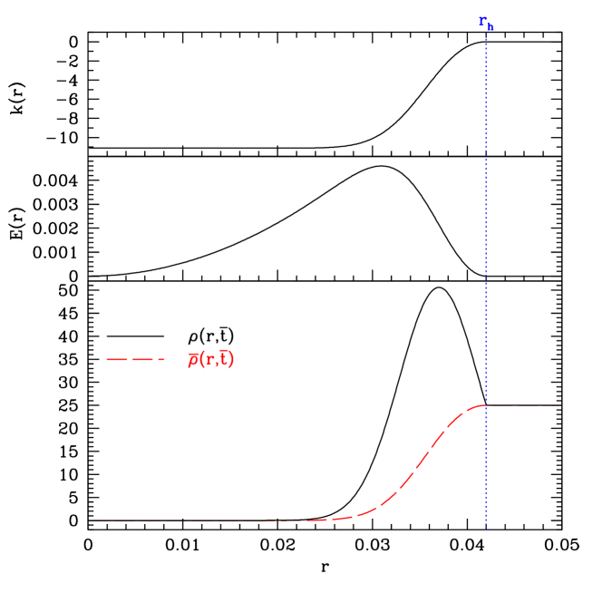
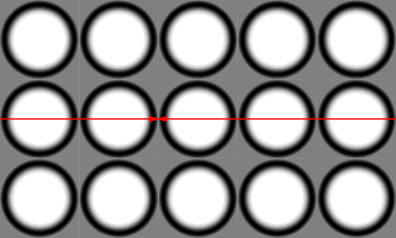
In Fig. 1 we plot the chosen Gaussian density profile. The hole ends at $r_{h}=0.042$, which is $350$ Mpc in size, roughly $25$ times smaller than $r_{BB}$. Note that this is not a very big bubble. But it is an almost empty region: in the interior the matter density is roughly $10^{4}$ times smaller than in the cheese. Our model consists of a sequence of five holes with the observer looking through them. The idea, however, is that the universe is completely filled with these holes, which form a sort of lattice. In this way an observer in the cheese will see an isotropic CMB along the two directions of sight shown in Fig. 2.

Figure 2: Sketch of our model. The shading mimics the initial density profile: darker shading implies larger denser. The uniform gray is the FRW cheese. The photons pass through the holes as shown by the arrows and are revealed by the observer placed in the cheese.

To have a realistic evolution, we demand that there are no initial peculiar velocities at time $\bar{t}$, i.e., that the initial expansion $H$ is independent of $r$. This implies

$$E(r)=\frac{1}{2}H_{FRW}^{2}(\bar{t})\,r^{2}-\frac{1}{6\pi}\frac{M(r)}{r}.$$ (8)

The function $E(r)$ chosen in this way is shown in Fig. 1. As seen from the figure, the curvature $E(r)$ is small compared with unity. In spite of its smallness, the curvature plays a crucial role to allow a realistic evolution of structures.

In Fig. 1 we also plot $k(r)=-2E(r)/r^{2}$, which is the generalization of the factor $k$ in the usual FRW models (it is not normalized to unity). As one can see, $k(r)$ is very nearly constant in the empty region inside the hole. This is another way to see the reason for our choice of the curvature function: we want to have in the center an empty bubble dominated by negative curvature.

II.3 The dynamics

Figure 3: Behavior of $Y(r,t)$ with respect to $r$, the peculiar velocities $v(r,t)$ with respect to $r$, and the density profiles $\rho(r,t)$ with respect to $r_{FRW}=Y(r,t)/a(t)$, for the curved case at times $t=\bar{t}=-0.8$, $t=-0.4$ and $t=t_{0}=0$. The straight lines for $Y(r,t)$ are the FRW solutions while the dashed lines are the LTB solutions. For the peculiar velocities, the matter gradually starts to move toward high density regions. The solid vertical line marks the position of the peak in the density with respect to $r$. For the densities, note that the curve for $\rho(r,0)$ has been divided by $10$. Finally, the values of $\rho(\infty,t)$ are $1,\ 2.8,$ and $25$, for $t=0,\ -0.4,\ -0.8$, respectively.

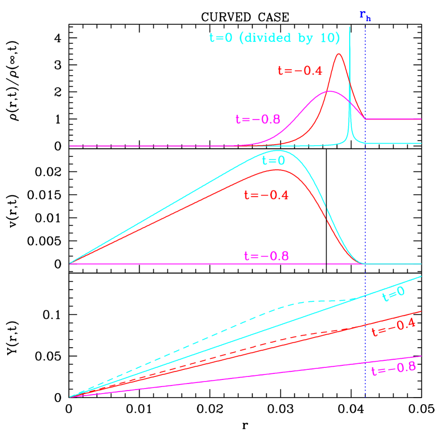
In Fig. 3 we show the evolution of $Y(r,t)$ for three times: $t=\bar{t}=-0.8$ (the Big Bang is at $t_{BB}=-1$), $t=-0.4$, and $t=0$ (corresponding to today). From Fig. 3 it is clear that outside the hole, i.e., for $r\geq r_{h}$, $Y(r,t)$ evolves as a FRW solution, $Y(r,t)\propto r$.

The inner almost empty region is expanding faster than the outer (cheese) region. The density ratio between the cheese and the interior region of the hole increases by a factor of $2$ between $t=\bar{t}$ and $t=0$. Initially the density ratio was $10^{4}$, but the model is not sensitive to this number since the evolution in the interior region is dominated by the curvature ($k(r)$ is much larger than the matter density).

The evolution is realistic, as one can see from Fig. 3, which shows the density profile at different times. Overdense regions start contracting and become thin shells (mimicking structures), while underdense regions become larger (mimicking voids), and eventually occupy most of the volume.

Let us explain why the high density shell forms and the nature of shell crossing. Because of the distribution of matter, the inner part of the hole is expanding faster than the cheese; between these two regions there is the initial overdensity. It is because of this that there is less matter in the interior part. (Remember that we matched the FRW density at the end of the hole.) Now we clearly see what is happening: the overdense region is squeezed by the interior and exterior regions, which act as a clamp. Shell crossing eventually happens when more shells—each labeled by its own $r$—are so squeezed that they occupy the same physical position $Y$, that is when $Y^{\prime}=0$. Nothing happens to the photons other than passing through more shells at the same time: this is the meaning of the $g_{rr}$ metric coefficient going to zero.

Remember that $r$ is only a label for the shell whose Euclidean position at time $t$ is $Y(r,t)$. In the plots of the energy density we have normalized $Y(r,t)$ using $r_{FRW}=Y(r,t)/a(t)$.

II.4 Redshift histories

Figure 4: Redshift histories for a photon that travels from one side of the five-hole chain to the other where the observer will detect it at present time. The dotted curve is for the FRW model. The vertical lines mark the edges of the holes. The plots are with respect to the coordinate radius $r$. Notice also that along the voids the redshift is increasing faster: indeed $z^{\prime}(r)=H(z)$ and the voids are expanding faster.

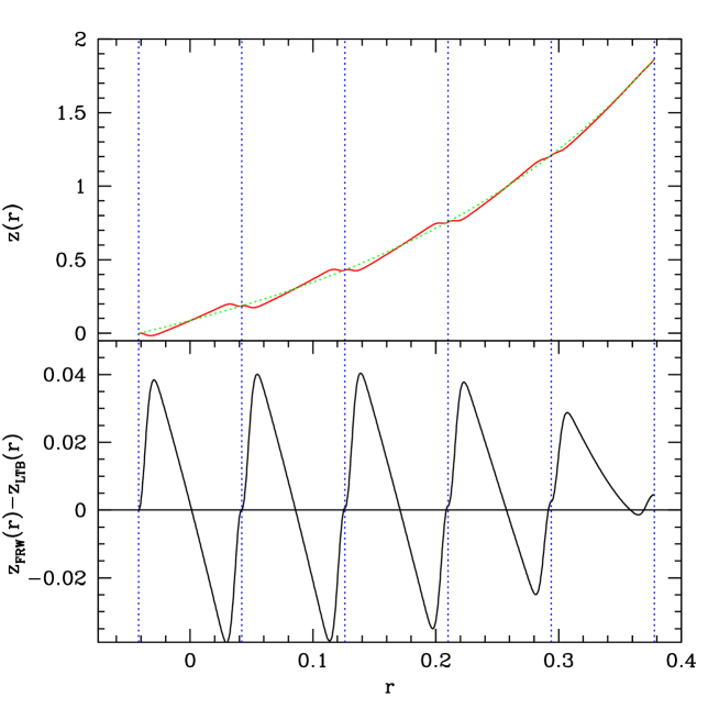
As shown in Fig. 4, this model does not feature substantial redshift effects: it is anyhow natural to expect a compensation, due to the spherical symmetry, between the incoming path and the outgoing path inside the same hole.

However, there is a compensation already on the scale of half a hole as it is clear from the plots. This mechanism is due to the density profile chosen, that is one whose average matches the FRW density of the cheese: roughly speaking we know that $z^{\prime}=H\propto\rho=\rho_{\scriptscriptstyle FRW}+\delta\rho$. We chose the density profile in order to have $\langle\delta\rho\rangle=0$, and therefore in its journey from the center to the border of the hole the photon will see a $\langle H\rangle\sim H_{\scriptscriptstyle FRW}$ and therefore there will be compensation for $z^{\prime}$.

Let us see this analytically. We are interested in computing a line average of the expansion along the photon path in order to track what is going on. Therefore, we shall not use the complete expansion scalar:

$$\theta=\Gamma_{0k}^{k}=2\frac{\dot{Y}}{Y}+\frac{\dot{Y}^{\prime}}{Y^{\prime}},$$ (9)

but, instead, only the part of it pertinent to a radial line average:

$$\theta_{r}=\Gamma_{01}^{1}=\frac{\dot{Y}^{\prime}}{Y^{\prime}}\equiv H_{r},$$ (10)

where $\Gamma_{0k}^{k}$ are the Christoffel symbols and $\theta$ is the trace of the extrinsic curvature.

Using $H_{r}$, we obtain:

$$\langle H_{r}\rangle=\frac{\int_{0}^{r_{h}}dr\;H_{r}\;Y^{\prime}/W}{\int_{0}^{r_{h}}dr\;Y^{\prime}/W}\simeq\left.\frac{\dot{Y}}{Y}\right|_{r=r_{h}}=H_{\scriptscriptstyle FRW},$$ (11)

where the approximation comes from neglecting the (small) curvature and the last equality holds thanks to the density profile chosen. This is exactly the result we wanted to find. However, we have performed an average at constant time and therefore we did not let the hole and its structures evolve while the photon is passing; the evolution of structures will partially break this compensation.

We have, therefore, seen that the compensation in redshift on the scale of half a hole is due to the density profile chosen. Even if we relax this requirement, we will still have a compensation on the scale of the hole. This can be seen in Fig. 4: inside each hole, the plot is anti-symmetric with respect to the center of the hole (the center of symmetry). This is only approximate at early times when structure evolution is fast enough to change the second half of the hole with respect to the first half.

This discussion sheds light on the fact that photon physics seems to be affected by the evolution of the inhomogeneities more than by the inhomogeneities themselves. We can argue that there should be perfect compensation if the hole will have a static metric such as the Schwarzschild one. In the end, this is a limitation of our assumption of spherical symmetry.

II.5 Luminosity and Angular-Diameter Distances

Figure 5: On the bottom the luminosity distance $d_{L}(z)$ in the five-hole model (jagged curve) and the $\Lambda$CDM solution with $\Omega_{M}=0.6$ and $\Omega_{DE}=0.4$ (regular curve) are shown. In the middle is the change in the angular diameter distance, $\Delta d_{A}(z)$, compared to a $\Lambda$CDM model with $\Omega_{M}=0.6$ and $\Omega_{DE}=0.4$. The top panel shows the distance modulus in various cosmological models. The jagged line is for the five-hole LTB model. The regular curves, from top to bottom, are a $\Lambda$CDM model with $\Omega_{M}=0.3$ and $\Omega_{DE}=0.7$, a $\Lambda$CDM model with $\Omega_{M}=0.6$ and $\Omega_{DE}=0.4$, the best smooth fit to the LTB model, and the EdS model. The vertical lines mark the edges of the five holes.

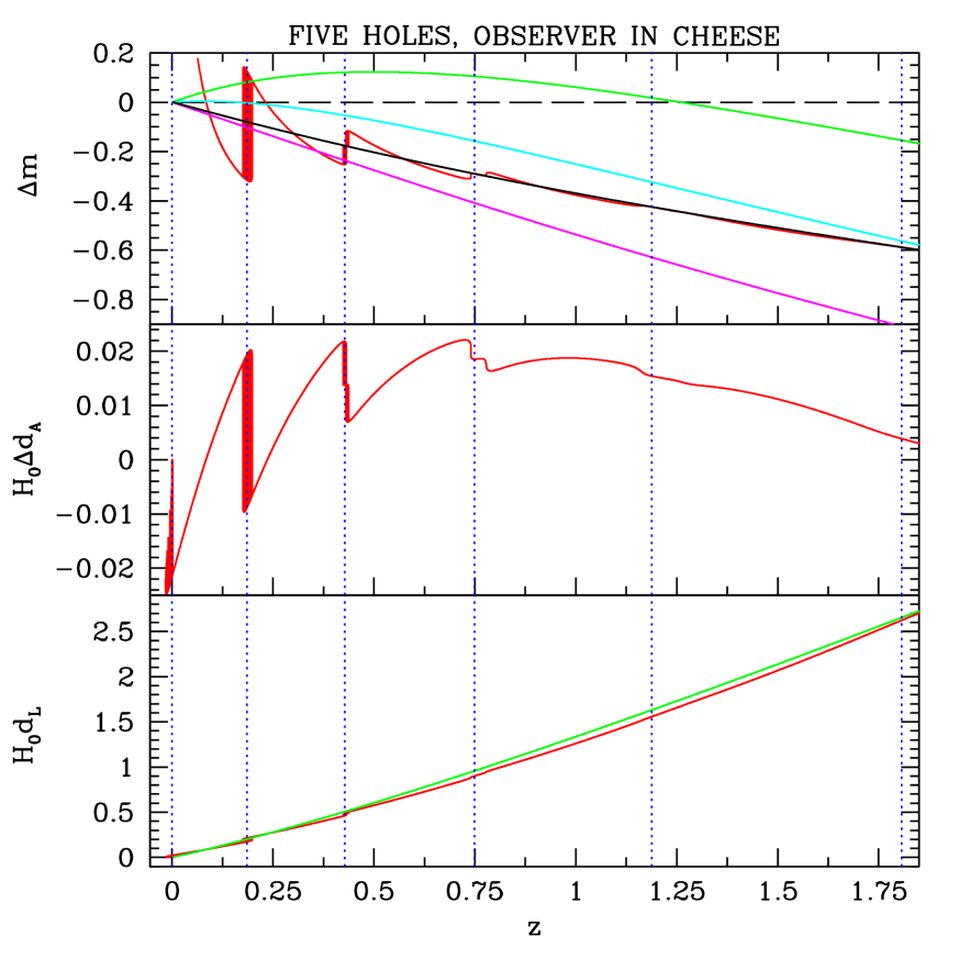
We show in Fig. 5 the results for the luminosity distance and angular distance. The solution is compared to the one of the $\Lambda$CDM model with $\Omega_{M}=0.6$ and $\Omega_{DE}=0.4$. It has an effective $q_{0}=\Omega_{M}/2-\Omega_{DE}=-0.1$.

The distance modulus is plotted in the top panel of Fig. 5. The solution shows an oscillating behavior that is due to the simplification of this toy model in which all the voids are inside the holes and all the structures are in thin spherical shells. For this reason a fitting curve was plotted: it is passing through the points of the photon path that are in the cheese between the holes. Indeed, they are points of average behavior and represent well the coarse graining of this oscillating curve. The simplification of this model tells us also that the most interesting part of the plot is farthest from the observer, let us say at $z>1$. In this region we can see the effect of the holes clearly: they move the curve from the EdS solution to the $\Lambda$CDM one with $\Omega_{M}=0.6$ and $\Omega_{DE}=0.4$. Of course, the model in not realistic enough to reach the “concordance” solution.

Summarizing, because of our assumption of spherical symmetry, we found no significant redshift effects. The effects we found came from the angular-diameter distance which is affected by the evolution of the inhomogeneities.

III The fitting problem

Now that we have seen how the luminosity-distance–redshift relation is affected by inhomogeneities, we want to study the same model from the point of view of light-cone averaging to see if we can gain insights into how inhomogeneities renormalize the matter swiss-cheese model and mimic a dark-energy component.

As explained in Ref. ellis-f , there are, broadly speaking, two distinct approaches that have been applied to understand the large-scale structure of the universe.

The standard approach is to make the assumption of spatial homogeneity and isotropy on a large enough scale, and to assume this guarantees that that the universe is represented by a FRW model. In other words, it is assumed that the dynamics of an inhomogeneous universe with density $\rho(\vec{x})$ is identical to the dynamics of a homogeneous universe of density $\langle\rho(\vec{x})\rangle$. The main problem with this approach is that it simplifies the way the real lumpy universe should be averaged. It does not really specify any type of averaging procedure necessary to make use of the FRW model, and it assumes that, in any case, the dynamics is not affected by inhomogeneities. Therefore, there is no information on what scales such a model is supposed to be applicable, if any.

The concordance model fits very well the experimental data: the direct consequence of its success is, indeed, that the isotropic and homogeneous $\Lambda$CDM model is a good phenomenological fit to the real inhomogeneous universe. And this is, in some sense, a reflection of the cosmological principle of spatial homogeneity and isotropy on a large enough scale: the inhomogeneous universe can be described by means of a isotropic and homogeneous solution. However this does not imply that a primary dark energy component really exists, but only that it exists effectively as far as the phenomenological fit is concerned. For example, it is not an observational consequence that the universe is globally accelerating (although it is usually stated as such). If primary dark energy does not exist, observational evidence coming from the concordance model would tell us that the pure-matter inhomogeneous model has been renormalized from the phenomenological point of view (e.g., the luminosity-distance and redshift of photons), into a homogeneous $\Lambda$CDM model.

The other approach is to make no a priori assumption of global symmetry, and build up our universe model only on the basis of astronomical observations. The main problem with the such an approach is the practical difficulty in implementing it.

An approach which is intermediate between the two outlined above is based on the fitting procedure. It asks the question about which FRW model best fits our lumpy universe. This question will lead to a procedure that will allow us to understand better how to interpret the large-scale FRW solution.

The best-fit procedure will be implemented along the past light cone. This is because a meaningful fitting procedure should be related directly to astronomical observations.

A remark is in order here: in the previous section we did not fit the $d_{L}(z)$ with an FRW solution. We have simply compared the shape of the $d_{L}(z)$ for the swiss-cheese model with the one of a $\Lambda$CDM model.

We intend now to fit a phenomenological FRW model to our swiss-cheese model. The FRW model we have in mind is a spatially flat model with a matter component with present fraction of the energy density $\Omega_{M}=0.25$, and with a phenomenological dark-energy component with present fraction of the energy density $\Omega_{\Lambda}=0.75$. We will assume that the dark-energy component has an equation of state

$$w(a)=w_{0}+w_{a}\left(1-\frac{a}{a_{0}}\right)=w_{0}+w_{a}\;\frac{z}{1+z}.$$ (12)

Thus, the total energy density in the phenomenological model evolves as

$$\frac{\rho^{\textrm{FIT}}}{\rho_{0}}=\Omega_{M}(1+z)^{3}+\Omega_{\Lambda}(1+z)^{3(1+w_{0}+w_{a})}\;\exp\left(-3w_{a}\frac{z}{1+z}\right).$$ (13)

We will refer to this model as the phenomenological model throughout this paper.

Our swiss-cheese model is a lattice of holes as sketched in Fig. 2: the scale of the inhomogeneities is therefore simply the size of a hole. We are interested in understanding how the equation of state of the “dark energy” in the phenomenological model changes with respect to $r_{h}$, and in particular, why. Of course, in the limit $r_{h}\rightarrow 0$, we expect to find $w=0$, that is, the underlying EdS model out of which the cheese is constructed.

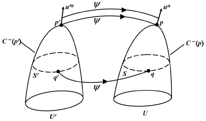
The procedure developed by Ref. ellis-f is summarized by Fig. 6. We refer the reader to that reference for a more thorough analysis and to Ref. Celerier:2007tp and references therein for recent developments. We will focus now in using our swiss-cheese model as (toy) cosmological model.

Figure 6: In the null data best fitting, one successively chooses maps from the real cosmological model $U$ to the FRW model $U^{\prime}$ of the null cone vertex $p^{\prime}$, the matter 4-velocity at $p^{\prime}$, a two-sphere $S^{\prime}$ on the null cone of $p^{\prime}$ and a point $q^{\prime}$ on the 2-sphere. This establishes the correspondence $\psi$ of points on the past null cone of $p^{\prime}$, $C^{-}(p^{\prime})$, to the past null cone of $p$, $C^{-}(p^{\prime})$, and then compares initial data at $q^{\prime}$ and at $q$. From Figure 2 of ellis-f .

III.1 Choice of vertex points

We start choosing the two observers to be compared. In the homogeneous FRW model every observer is the same thanks to spatial homogeneity. We choose an observer in the cheese as the corresponding observer in our swiss-cheese model, in particular the one shown in Fig. 2.

Our model allows us to choose also the time of observation, which, in general, is a final product of the comparison. We now explain why.

The FRW model we will obtain from the fit will evolve differently from the swiss cheese: the latter evolves as an EdS model, while the former will evolve as a quintessence-like model. They are really different models. They will agree only along the light cone, that is, on our observations.

Now, for consistency, when we make local measurements the two models have to give us the same answer: local measurements indeed can be seen as averaging measurements with a small enough scale of averaging, and the two models agree along the past light cone.

Therefore, we choose the time in order that the two observers measure the same local density. This feature is already inherent in Eq. (13): the phenomenological model and the swiss-cheese model evolve in order to have the same local density, and therefore the same Hubble parameter, at the present time.

III.2 Fitting the 4-velocity

The next step is to fit the four-velocities of the observers. In the FRW model we will choose a comoving observer, the only one who experiences an isotropic CMB. In the swiss-cheese model, we will choose, for the same reason, a cheese-comoving observer. Again, our swiss-cheese model considerably simplifies our work.

III.3 Choice of comparison points on the null cones

Now that the past null cones are uniquely determined, we have to choose a measure of distance to compare points along each null cone.

First, let us point out that instead of the entire two-sphere along the null cone, we will examine, only a point on it. This is because of the simplified set-up of our swiss-cheese model in which the observer is observing only in two opposite directions, as illustrated in Fig. 2. This means that we can skip the step consisting in averaging our observable quantities over the surface of constant redshift, which generally is necessary in order to be able to compare an inhomogeneous model with the FRW model ellis-f .

Coming back to the main issue of this section, we will use the observed redshift $z$ to compare points along the null cones. Generally, the disadvantage of using it is that it does not directly represent distances along the null cone. Rather, the observed value $z$ is related to the cosmological redshift $z_{C}$ by the relation:

$$1+z=(1+z_{O})(1+z_{C})(1+z_{S})$$ (14)

where $z_{O}$ is the redshift due to the peculiar velocity of the observer $O$ and $z_{S}$ that due to the peculiar velocity of the source. The latter, in particular, is a problem because local observations cannot distinguish $z_{S}$ from $z_{C}$.

However, our set up again simplifies this task. The observers chosen are, indeed, both comoving (in the swiss-cheese model because the observer is in the cheese, and in the phenomenological model by construction), and therefore $z_{O}=0$. Regarding the sources, we know exactly their behavior because we have a model to work with.

The sources are also comoving; however, there are structure-formation effects that should be disentangled from the average evolution. For this reason we will perform averages between points in the cheese (the meaning of this will be clear in the next section) in order to smooth out these structure-formation effects.

III.4 Fitting the null data

Figure 7: An illustration of the points chosen for the averaging procedure.

Now we are ready to set up the fitting of our swiss-cheese model. Ref. Hellaby:1988zz studied the approach based on volume averaging outlined in Ref. ellis-f . This approach, however, is appropriate for studies concerning global dynamics, as in Refs. carfora ; buchert_new . As stressed previously, here we are instead interested in averages directly related to observational quantities, and we constructed our model following this idea: it is a model that is exactly solvable and “realistic” (even if still toy) at the price of no interesting volume-averaged dynamics.

Therefore, we will follow a slightly different approach from the ones outlined in Ref. ellis-f : we are going to fit averages along the light cone. This method will be intermediate between the fitting approach and the averaging approach.

We will focus on the expansion scalar and the density. We will see that these two quantities behave differently under averaging. We denote by $Q^{\textrm{SC}}(r,t)$ a quantity in the swiss-cheese model we want to average. We denote by $Q^{\textrm{FIT}}(t)$ the corresponding quantity we want to fit to the average of $Q^{\textrm{SC}}(r,t)$. Note that $Q^{\textrm{FIT}}(t)$ does not depend on $r$ because the phenomenological model we will employ to describe the swiss-cheese model is homogeneous.

Again, the fit model is a phenomenological homogeneous model (just refereed to as the phenomenological model). It need not be the model of the cheese.

The procedure is as follows. First we will average $Q^{\textrm{SC}}(r,t)$ for a photon that starts from the emission point $E$ of the five-hole chain and arrives at the locations of observers $O_{i}$ of Fig. 7. We have chosen those points because they well represent the average dynamics of the model. Indeed, these points are not affected by structure evolution because they are in the cheese. Then, we will compare this result with the average of $Q^{\textrm{FIT}}(t)$ for the phenomenological and homogeneous source with density given by Eq. (13) with an equation of state $w$ given by Eq. (12).

The two quantities to be compared are therefore:

$$\langle Q^{\textrm{SC}}\rangle_{\overline{\scriptscriptstyle EO}_{i}} = \left[\int_{E}^{O_{i}}dr\;Y^{\prime}/W\right]^{-1}\int_{E}^{O_{i}}dr\ Q^{\textrm{SC}}(r,t(r))\;Y^{\prime}(r,t(r))/W(r)$$

$$\langle Q^{\textrm{FIT}}\rangle_{\overline{\scriptscriptstyle EO}_{i}} = \left[\int_{E}^{O_{i}}dr\;a_{\scriptscriptstyle FIT}\right]^{-1}\int_{E}^{O_{i}}dr\ Q^{\textrm{FIT}}(t_{\scriptscriptstyle FIT}(r))\;a_{\scriptscriptstyle FIT}(t_{\scriptscriptstyle FIT}(r)),$$ (15)

where $t(r)$ and $t_{\scriptscriptstyle FIT}(r)$ are the photon geodesics in the swiss-cheese model and in the phenomenological one, respectively. The functions $t_{\scriptscriptstyle FIT}(r)$, $a_{\scriptscriptstyle FIT}$ and other quantities we will need are obtained solving the Friedman equations with a source described by Eq. (13) with no curvature. The points $O_{i}$ in the swiss-cheese model of Fig. 7 are associated to points in the phenomenological model with the same redshift, as discussed in Sec. III.3.

We will then find the $w$ that gives the best fit between $\langle Q^{\textrm{FIT}}\rangle$ and $\langle Q^{\textrm{SC}}\rangle$, that is, the choice that minimizes:

$$\sum_{i}\left(\langle Q^{\textrm{FIT}}\rangle_{\overline{\scriptscriptstyle EO}_{i}}-\langle Q^{\textrm{SC}}\rangle_{\overline{\scriptscriptstyle EO}_{i}}\right)^{2}.$$ (16)

Of course, in the absence of inhomogeneities, this method would give $w=0$.

Let us summarize the approach:

• We choose a phenomenological quintessence-like model that, at the present time, has the same density and Hubble parameter as the EdS-cheese model.

• We make this phenomenological model and the swiss-cheese model correspond along the light cone via light-cone averages of $Q$.

• We can substitute the swiss-cheese model with the phenomenological model as far as the averaged quantity $Q$ is concerned.

The ultimate question is if it is observationally meaningful to consider $Q$, as opposed to the other choice of domain averaging at constant time, which is not directly related to observations. We will come back to this issue after having obtained the results.

III.4.1 Averaged expansion

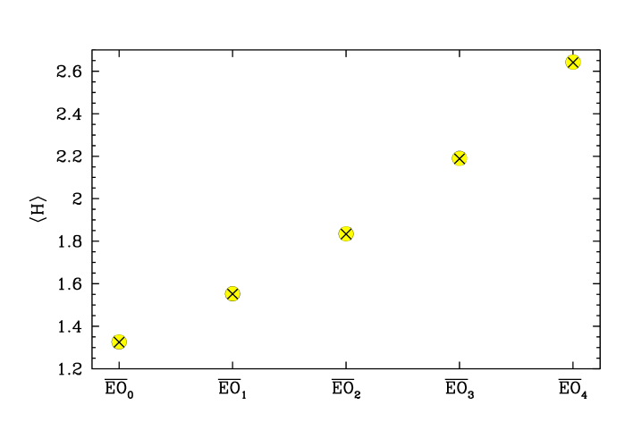
The first quantity in which we are interested is the expansion rate. To average the expansion rate we will follow the formalism developed in Sec. II.4. We will therefore apply Eqs. (15-16) to $Q^{\textrm{SC}}=H_{r}\equiv\dot{Y}^{\prime}/Y^{\prime}$, where we remember that $H_{r}$ is the radial expansion rate. The corresponding quantity in the phenomenological model is $Q^{\textrm{FIT}}=\dot{a}_{\scriptscriptstyle FIT}/a_{\scriptscriptstyle FIT}$.

For the same reason there is good compensation in redshift effects (see Sec. II.4), we expect $\langle H_{r}\rangle$ to behave very similarly to the FRW cheese solution. Indeed, as one can see in Fig. 8, the best fit of the swiss-cheese model is given by an phenomenological source with $w\simeq 0$, that is, the phenomenological model is the cheese-FRW solution itself as far as the expansion rate is concerned.

Figure 8: Average expansion rate. The yellow points are $\langle H^{\textrm{SC}}\rangle_{\overline{\scriptscriptstyle EO}_{i}}$ while the crosses are $\langle H^{\textrm{FIT}}\rangle_{\overline{\scriptscriptstyle EO}_{i}}$. $\overline{EO}_{i}$ means that the average was performed from $E$ and $O_{i}$ with respect to Fig. 7. The best fit is found for $w\simeq 0$, that is, the phenomenological model is the cheese-FRW solution itself as far as the expansion rate is concerned.

III.4.2 Averaged density

The situation for the density is very different. The photon is spending more and more time in the (large) voids than in the (thin) high density structures. We apply Eqs. (15-16) to $Q^{\textrm{SC}}=\rho^{\textrm{SC}}$. The corresponding quantity in the phenomenological model is $Q^{\textrm{FIT}}=\rho^{\textrm{FIT}}$ where $\rho^{\textrm{FIT}}$ is given by Eq. (13). The results are illustrated in Fig. 9: the best fit is for $w_{0}=-1.95$ and $w_{a}=4.28$.

Figure 9: Average density in $\rho_{C0}$ units. The yellow points are $\langle\rho^{\textrm{SC}}\rangle_{\overline{\scriptscriptstyle EO}_{i}}$ while the crosses are $\langle\rho^{\textrm{FIT}}\rangle_{\overline{\scriptscriptstyle EO}_{i}}$. $\overline{EO}_{i}$ means that the average was performed from $E$ and $O_{i}$ with respect to Fig. 7. The parametrization of $\rho^{\textrm{FIT}}$ is from Eq. (13). The best fit is found for $w_{0}=-1.95$ and $w_{a}=4.28$.

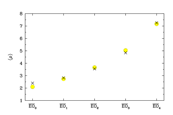
As we will see in Sec. V, we can achieve a better fit to the concordance model with smaller holes than the ones of $350$ Mpc considered here. We anticipate that for a holes of radius $r_{h}=250$ Mpc, we have $w_{0}=-1.03$ and $w_{a}=2.19$.

We see, therefore, that this swiss-cheese model could be interpreted, in the FRW hypothesis, as a homogeneous model that is initially dominated by matter and subsequently by dark energy: this is what the concordance model suggests. We stress that this holds only for the light-cone averages of the density.

IV Discussion

IV.1 Explanation

Let us first explore the basis for what we found. In Fig. 10 we show the density along the light cone for both the swiss-cheese model and the EdS model for the cheese. It is clear that the photon is spending more and more time in the (large) voids than in the (thin) high density structures.

Figure 10: Density along the light-cone for the swiss-cheese model (the spiky curve) and the EdS model of the cheese (the regular curve). The labeling of the $x$-axis is the same one of Fig. 7.

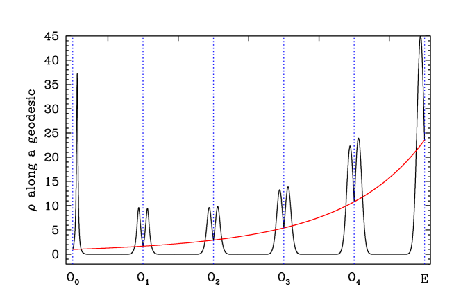
To better show this, we plotted in Fig. 11 the constant-time, line-averaged density as a function of time. The formula used for the swiss-cheese model is

$$\int_{0}^{r_{h}}dr\ \rho(r,t)\;Y^{\prime}(r,t)/W(r)\left/\int_{0}^{r_{h}}dr\;Y^{\prime}/W\right.,$$ (17)

while for the cheese, because of homogeneity we can just use $\rho(t)$ of the EdS model. As one can see, the photon is encountering less matter in the swiss-cheese model than in the EdS cheese model. Moreover, this becomes increasingly true with the formation of high-density regions as illustrated in Fig. 11 by the evolution of the ratio of the previously calculated average density: it decreases by $17\%$ from the starting to the ending time.

Figure 11: At the top is the evolution of the energy density for the Eds cheese model (higher curve) and for the phenomenological model with $w_{0}=-1.95$ and $w_{a}=4.28$. In the middle is the constant-time line averaged density as a function of time for the swiss-cheese model (lower curve) and the cheese-EdS model (higher curve). At the bottom is their ratio of the last two quantities as a function of time.

The calculation of Eq. (17) is actually, except for some factors like the cross-section, the opacity of the swiss-cheese model. Therefore, a photon propagating through the swiss-cheese model has a different average absorption history; that is, the observer looking through the cheese will measure a different flux compared to the case with only cheese and no holes. For the moment, in order to explore the physics, let us make the approximation that during the entire evolution of the universe, the matter is transparent to photons.

From the plots just shown we can now understand the reason for the best fit values of $w_{0}=-1.95$ and $w_{a}=4.28$ found in the case of holes of $r_{h}=350$ Mpc. We are using a homogeneous phenomenological model, which has at the present time the density of the cheese (see Fig. 11). We want to use it to fit the line-averaged density of the swiss cheese, which is lower than the (volume) averaged one. Therefore, going backwards from the present time, the phenomenological model must keep its density low, that is, to have a small $w$. At some point, however, the density has to start to increase, otherwise it will not match the line-averaged value that keeps increasing: therefore $w$ has to increase toward $0$. It is very interesting that this simple mechanism mimics the behavior of the concordance-model equation of state. We stress that this simple mechanism works thanks to the set-up and fitting procedure we have chosen; that is, the fact that we matched the cheese-EdS solution at the border of the hole, the position of the observer, and the observer looking through the holes. Moreover, we did not tune the model to achieve a best matching with the concordance model. The results shown are indeed quite natural.

IV.2 Beyond spherical symmetry

In this work we are interpreting the swiss-cheese model from the point of view of light-cone averages. In Ref. marra-sc we have instead focused on the luminosity-distance–relation (see Fig. 5).

Figure 12: Flow chart regarding relationships between the results obtained in Ref. marra-sc and this work See Sec. IV.2 for a discussion.

We have summarized the relationships between the results obtained in Ref. marra-sc and this work in the flow chart of Fig. 12.

Regarding $d_{L}(z)$, we found no important effects from a change in the redshift: the effects on $d_{L}(z)$ all came from $d_{A}$ driven by the evolution of the inhomogeneities.

Regarding light-cone averages, we found no important effects with respect to the expansion: this negative result is due to the compensation in redshift discussed in Sec. II.4 and it is the same reason why we did not find redshift effects with $d_{L}(z)$. This is the main limitation of our model and it is due ultimately to the spherical symmetry of the model as explained in Sec. II.4.

We found important effects with respect to the density: however this is not due to the effects driving the change in $d_{A}$. The latter is due to structure evolution while the former to the presence of voids, so the two causes are not directly connected. Indeed, it is possible to turn off the latter and not the former.

We can therefore make the point that the expansion is not affected by the inhomogeneities because of the compensation due to the spherical symmetry. The density, on the other hand, is not affected by the spherical symmetry, so there are no compensations, and the photon systematically sees more and more voids than structures. We can therefore argue that the average of the density is more relevant than the average of the expansion because it is less sensitive to the assumption of spherical symmetry, which is one of the limitations of this model.

The next step is to define a Hubble parameter from this average density: $H^{2}\propto\langle\rho\rangle_{\gamma}$. In this way we are moving from a swiss cheese made of spherically symmetric holes to a swiss cheese without exact spherical symmetry. The correspondence is through the light-cone averaged density which, from this point of view, can be seen as a tool in performing this step.

Summarizing again:

• We started with a swiss-cheese model containing only spherically symmetric holes. A photon, during its journey through the swiss cheese, undergoes a redshift that is not affected by inhomogeneities. However the photon is spending more and more time in the voids than in the structures. The lack of an effect is due to spherical symmetry. We focus on this because a photon spending most of its time in voids should have a different redshift history than a photon propagating in a homogeneous background.

• Since the density is a quantity that is not particularly sensitive to spherical symmetry, we try to resolve the mismatch by focusing on the density alone and getting from it the expansion (and therefore the redshift history).

• We ended up with a swiss-cheese model with holes that effectively are not spherically symmetric. In this model there is an effect on the redshift history of a photon due to the voids.

• In practice this means that we will use the phenomenological best-fit model found, that is, we will use a model that behaves similarly to the concordance model.

IV.3 Motivations

Let us go back to the discussion of Sec. III.4, that is, if it is observationally meaningful to consider light-cone averages of $Q$ as the basis for the correspondence. For example, domain averages at constant time are not directly related to observations.

Here, we are not claiming that light-cone averages are observationally relevant. Rather, we are using light-cone averages as tools to understand the model at hand. The approach has been explained in the previous section.

V Renormalization of the matter equation of state

In this section we will study how the parameters of the phenomenological model depend on the size of the inhomogeneities, that is, on the size of the hole. We sketched in Fig. 13 our set-up: we keep the comoving position of the centers of the holes fixed. The observer is located in the same piece of cheese.

Figure 13: Sketch of how the size of the inhomogeneity is changed in our model. The shading mimics the initial density profile: darker shading implies larger denser. The uniform gray is the FRW cheese. The photons pass through the holes as shown by the arrows and are revealed by the observer whose comoving position in the cheese does not change. The size of the holes correspond to $n=0,$ $2$, $5$ of Eq. (18).

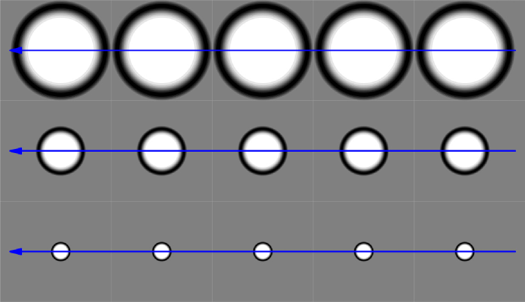
We changed the radius of the hole according to

$$r_{h}(n)=\frac{r_{h}}{1.4^{n}},$$ (18)

where $r_{h}$ is the radius we have been using till now, the one that results in the holes touching. The choice of the $1.4$ in the scaling is only for convenience. We let $n$ run from $0$ to $7$.

In this analysis we will use instead of the energy density in Eq. (13), an energy density in which only one effective source appears, and the effective source evolves as

$$\frac{\rho^{\textrm{FIT}}}{\rho_{0}}=(1+z)^{3(1+w^{R}_{0}+w^{R}_{a})}\;\exp\left(-3w^{R}_{a}\frac{z}{1+z}\right)\qquad\mbox{with}\qquad w^{R}(z)=w^{R}_{0}+w^{R}_{a}\;\frac{z}{1+z}.$$ (19)

We put $R$ as a superscript on the equation of state in order to differentiate the parametrization of Eq. (19), which we are now using to study the renormalization, from the parametrization of Eqs. (12-13), which we used to compare the phenomenological model to the concordance model. We are not disentangling different sources in Eq. (19) because we are interested in the renormalization of the matter equation of state of the cheese, that is, on the dependence of $w^{R}$ upon the size of the hole. To this purpose we need only one source in order to keep track of the changes.

As one can see from Fig. 14, we have verified that $w^{R}=0$ for $r_{h}\rightarrow 0$, i.e., we recover the EdS model as the best-fit phenomenological model.

We are interested to see if the equation of state exhibits a power-law behavior and, therefore, we use the following functions to fit $w^{R}_{0}$ and $w^{R}_{a}$:

$$\frac{w^{R}_{0}(n)}{w^{R}_{0}(0)} = q_{0}\left(\frac{r_{h}(n)}{r_{h}(0)}\right)^{p_{0}}$$

$$\frac{w^{R}_{a}(n)}{w^{R}_{a}(0)} = q_{a}\left(\frac{r_{h}(n)}{r_{h}(0)}\right)^{p_{a}}.$$ (20)

We performed a fit with respect to the logarithm of the above quantities, the result is shown in Fig. 14. We found:

$$p_{0} = p_{a}\simeq 1.00$$

$$q_{0} = q_{a}\simeq 0.88.$$ (21)

Figure 14: At the top, dependence of $w^{R}_{0}$ (lower points denoted by circles) and $w^{R}_{a}$ (upper points denoted by $\times$) with respect of the size of the hole. At the bottom, fit as explained in the text. Recall that $r_{h}$ is today $350$ Mpc.

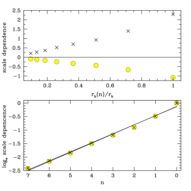
Summarizing, we found three important facts.

• The parameters of the equation of state as a function of the size of the hole exhibit a power-law behavior.

• The power-laws of $w^{R}_{0}$ and $w^{R}_{a}$ have the same scaling exponent. This is actually a check: once a physical quantity exhibits a power-law behavior, we expect that all its parameters share the same scaling exponent.

• The scale dependence is linear: the equation of state depends linearly on the length of holes the photon propagates through. We stress that the dependence we are talking about is not on the scale of the universe, but on the size of the holes.

We can finally ask which size of the holes will give us a phenomenological model able to mimic the concordance model. We found that for $n=1$, that is for a holes of radius $r_{h}=250$ Mpc, we have $w^{R}_{0}=1.4$ and $w^{R}_{a}=-0.665$, which in terms of the energy density parametrization of Eq. (13), corresponds to $w_{0}=-1.03$ and $w_{a}=2.19$.

VI Conclusions

The aim of this investigation was to understand the role of large-scale non-linear cosmic inhomogeneities in the interpretation of observational data. We focused on an exact (if toy) solution, based on the Lemaître-Tolman-Bondi (LTB) model. This solution has been studied extensively in the literature alnes0607 ; notari-mansouri ; alnes0602 ; celerier ; mansouri ; flanagan ; rasanen ; tomita ; chung ; nambu . It has been shown that it can be used to fit the observed $d_{L}(z)$ without the need of dark energy (for example in Ref. alnes0602 ). To achieve this result, however, it is necessary to place the observer at the center of a rather large-scale underdensity. To overcome this fine-tuning problem we built a swiss-cheese model, placing the observer in the cheese and having the observer look through the holes in the swiss-cheese as pictured in Fig. 2.

In Sec. II we defined the model and described its dynamics: it is a swiss-cheese model where the cheese is made of the usual FRW solution and the holes are made of a LTB solution. The voids inside the holes are expanding faster than the cheese. We reported also the results for $d_{L}(z)$ obtained in Ref. marra-sc , to which we refer the reader for a more thorough analysis. We found that redshift effects are suppressed because of a compensation effect due to spherical symmetry. However, we found interesting effects in the calculation of the angular distance: the evolution of the inhomogeneities bends the photon path compared to the FRW case. Therefore, inhomogeneities will be able (at least partly) to mimic the effects of dark energy.

After having analyzed the model from the observational point of view, we set up in Section III the fitting problem in order to better understand how inhomogeneities renormalize the matter swiss-cheese model allowing us to eschew a primary dark energy. We followed the scheme developed in Ref. ellis-f , but modified in the way to fit the phenomenological model to the swiss-cheese one. We chose a method that is intermediate between the fitting approach and the averaging one: we fitted with respect to light-cone averages.

In particular, we focused on the expansion and the density. While the expansion behaved as in the FRW case because of the compensation effect mentioned above, we found that the density behaved differently thanks to its intensiveness to that compensation effect: a photon is spending more and more time in the (large) voids than in the (thin) high density structures. This effect is not directly linked to the one giving us an interesting $d_{A}$. The best fit we found for holes of $r_{h}=250$ Mpc is $w_{0}=-1.03$ and $w_{a}=2.19$; qualitatively similar to the concordance model.

The flow chart of Fig. 12 summarizes the results obtained. The insensitivity to the compensation effect made us think that a swiss cheese made of spherical symmetric holes and a swiss cheese without an exact spherical symmetry would share the same light-cone averaged density. Knowing the behavior of the density we are therefore able to know the one of the Hubble parameter that will be the one of the FRW solution with an phenomenological source characterized by the fit equation of state. In this way we can think to go beyond the main limitation of this model, that is, the assumption of spherical symmetry. From this point of view, the light-cone averaged density can be seen as a tool in performing this step.

Summarizing:

• We started with a swiss-cheese model based on spherically symmetric holes. A photon, during its journey through the swiss cheese, undergoes a redshift which is not affected by inhomogeneities. However the photon is spending more and more time in the voids than in the structures. The lack of an effect is due to the the assumption of spherical symmetry. We focus on this because a photon spending most of its time in voids should have a different redshift history than a photon propagating in a homogeneous background.

• Assuming that the density is a quantity that does not heavily depend on the assumption of spherical symmetry, we tried to resolve the issue by focusing on the density alone and getting from it the expansion (and therefore the redshift history).

• This resulted in a swiss-cheese model with holes that effectively are not perfectly spherical. In this model the redshift history of a photon depends on the time passed inside the voids.

• In practice this means that we will use the phenomenological best-fit model found, that is, we will use a model that behaves similarly to the concordance model.

Then, in Section V we studied how the equation of state of a phenomenological model with only one effective source depends on the size of the inhomogeneity. We found that $w^{R}_{0}$ and $w^{R}_{a}$ follow a power-law dependence with the same scaling exponent which is equal to unity. That is, the equation of state depends linearly on the distance the photon travels through voids.

We finally asked which size of the holes will give us a phenomenological model able to mimic the concordance model. We found that for $n=1$, that is for a holes of radius $r_{h}=250$ Mpc, we have $w_{0}=-1.03$ and $w_{a}=2.19$.