The imprints of primordial non-gaussianities on large-scale structure: scale dependent bias and abundance of virialized objects
Abstract
We study the effect of primordial nongaussianity on large-scale structure, focusing upon the most massive virialized objects. Using analytic arguments and N-body simulations, we calculate the mass function and clustering of dark matter halos across a range of redshifts and levels of nongaussianity. We propose a simple fitting function for the mass function valid across the entire range of our simulations. We find pronounced effects of nongaussianity on the clustering of dark matter halos, leading to strongly scale-dependent bias. This suggests that the large-scale clustering of rare objects may provide a sensitive probe of primordial nongaussianity. We very roughly estimate that upcoming surveys can constrain nongaussianity at the level , competitive with forecasted constraints from the microwave background.
I Introduction
One of the fundamental predictions of standard (single-field, slow-roll) inflationary cosmology is that the density fluctuations in the early universe that seeded large-scale structure formation were nearly gaussian random (e.g. Maldacena (2003); Acquaviva et al. (2003); Creminelli (2003); Lyth and Rodriguez (2005a); Seery and Lidsey (2005)). Constraining or detecting non-gaussianity (NG) is therefore an important and basic test of the cosmological model. To the extent that it can be measured, gaussianity has so far been confirmed; the tightest existing constraints have been obtained from observations of the cosmic microwave background Spergel et al. (2007); Creminelli et al. (2007a). Recently, several inflationary models have been proposed which predict a potentially observable level of nongaussianity, see e.g. Arkani-Hamed et al. (2004); Bartolo et al. (2004a); Lyth and Rodriguez (2005b); Rigopoulos et al. (2006); Allen et al. (2006); Chen (2005); Barnaby and Cline (2006); Barnaby and Cline (2007a, b); Sasaki et al. (2006); Chen et al. (2007a, b); Battefeld and Easther (2007); Assadullahi et al. (2007); Battefeld and Battefeld (2007); Bean et al. (2007) and Bartolo et al. (2004b) for a review. Improved limits on NG would rule out some of these models; conversely, a robust detection of primordial nongaussianity would dramatically overturn standard inflationary cosmology and provide invaluable information about the nature of physical processes in the early universe. In this regard, there has been a resurgence in studying increasingly more sophisticated methods and algorithms to constrain (or, if we are lucky, detect) nongaussianity Babich (2005); Babich et al. (2004); Creminelli et al. (2007b); Smith and Zaldarriaga (2006a); Fergusson and Shellard (2006).
Nongaussianity manifests itself not only in the cosmic microwave background Falk et al. (1993); Luo and Schramm (1993); Gangui et al. (1994); Wang and Kamionkowski (2000), but also in the late-time evolution of large-scale structure. For example, detailed measurements of higher order correlations like the bispectrum or trispectrum of galaxy clustering could provide a handle on primordial nongaussianity Verde et al. (2001); Scoccimarro et al. (2004); Sefusatti and Komatsu (2007). The abundance of galaxy clusters, the largest virialized objects in the universe, has also long been recognized as a sensitive probe of primordial NG Lucchin and Matarrese (1988); Robinson and Baker (1999); Benson et al. (2002); Matarrese et al. (2000); Verde et al. (2001); Scoccimarro et al. (2004); Komatsu et al. (2003). Because clusters are rare objects which form from the largest fluctuations on the tails of the density probability distribution, their abundance is keenly sensitive to changes in the shape of the PDF such as those caused by nongaussianity. Large statistical samples of massive clusters have already been compiled from wide-area optical imaging and spectroscopic surveys such as the Sloan Digital Sky Survey Rozo et al. (2007); Koester et al. (2007), the Two-Degree Survey Eke et al. (2004), and from the Red Sequence Survey Yee et al. (2007) and from X-ray surveys using the Chandra and XMM-Newton observatories Willis et al. (2005); Valtchanov et al. (2004). Future missions, such as the Dark Energy Survey, Supernova/Acceleration Probe and Large Synoptic Survey Telescope, will detect and study tens of thousands of clusters, revolutionizing our understanding of cluster physics as well as providing important constraints on cosmology Haiman et al. (2001); Majumdar and Mohr (2003); Wang et al. (2004); Battye and Weller (2005); Lima and Hu (2005); Marian and Bernstein (2006); Takada and Bridle (2007).
To exploit the potential of these upcoming surveys as probes of primordial nongaussianity, it is important to calibrate the effects of NG on the abundance and clustering of virialized objects. While no previous work has attempted to quantify the effects of NG on halo clustering, several groups over the past decade have constructed fitting formulae for the halo mass function Robinson and Baker (2000); Robinson et al. (2000); Matarrese et al. (2000). All of this work, however, was analytic and relied on the validity of the Press-Schechter Press and Schechter (1974) formalism, plus various further approximations. The resulting analytic estimates are, in general, rather cumbersome to compute and have questionable accuracy. As discussed below, the Press-Schechter model provides only a qualitative description of halo abundance, and fails to reproduce the halo mass function to within an order of magnitude over the mass and redshift range accessible to current and future cluster surveys. Therefore, analytic models for NG cluster abundance based on the Press-Schechter ansatz may not be sufficiently accurate. Given the high-quality data soon to be available, a much more precise calculation of cluster statistics will be required. Quite recently, two groups have attempted to quantify the mass function of clusters in NG models using N-body simulations Kang et al. (2007); Grossi et al. (2007), reaching contradictory conclusions.
In this paper, we use analytic arguments and numerical simulations to estimate the effect of NG on the abundance and clustering of virialized objects. Because N-body simulations can be expensive and there is a wide NG parameter space, we also strive to make our results useful to a cosmologist who is not necessarily equipped with the machinery or patience to run simulations or evaluate difficult analytic expressions. To this end, we provide a simple, physically motivated fitting formula for the halo mass function and halo bias, which we calibrate to our N-body simulations.
Our main results are that the mass function and correlation function of massive halos can be significantly modified by primordial nongaussianity. We find a somewhat weaker effect of NG on the mass function than previous analytic estimates. We also show analytically and numerically that NG strongly affects the clustering of rare objects on large scales, implying that measurements of the large-scale power spectrum can place stringent bounds on NG.
The plan of the paper is as follows. In Section II we derive analytic expressions for the abundance and clustering of rare peaks. In Section III we describe our N-body simulations, followed in Section IV by a discussion of our measured halo mass function, and our fitting formula for the mass function. In Section V we present measurements of halo clustering within our simulations, and in Section VI we discuss cosmological implications of our findings.
II Analytic estimates
In this section, we derive analytic expressions for the abundance and clustering of dark matter halos. As mentioned above, such analytic approaches provide a useful qualitative framework for understanding gravitational collapse, however they cannot be used to describe quantitatively either the mass function or the clustering amplitude of collapsed objects. The expressions derived here are meant solely to motivate the more precise fitting formulae described in subsequent sections.
We will focus on local NG of the form Matarrese et al. (2000); Komatsu and Spergel (2001); Maldacena (2003)
| (1) |
In our notation, , where is the usual Newtonian potential. On subhorizon scales, this choice of Newtonian gauge is valid, and the potentials and satisfy the Poisson equation relating them to the overdensity . On superhorizon scales, the Bardeen potential and overdensity are proportional, and not related by a Poisson equation, so our analysis will be valid only on subhorizon scales. With this choice of convention, positive corresponds to positive skewness of the density probability distribution, and hence an increased number of massive objects.
For simplicity, we neglect the effect of the CDM transfer functions, which modify the shape of the power spectrum after nongaussianity is generated. Then the probability distribution for is easy to write down, however the probability distribution for the density cannot be expressed analytically. Nevertheless, we can make progress by assuming that the NG correction is small, and by focusing only on high peaks of the density. The Laplacian of is
| (2) |
Because , , and are all Gaussian fields whose statistics are fully specified by their power spectra, then Eqn. (2) above, relating to the Gaussian fields, allows us to determine fully the statistics of the nongaussian density . For example, the skewness of becomes, to lowest order in ,
| (3) |
On the average, the two terms and in Eqn. (2) are of the same order; the fact that they have equal but opposite expectation value is why . However we are mainly interested in high peaks, where is large. Because is uncorrelated with , and because at the peak of its derivative vanishes, we assume that may be neglected compared to in the vicinity of rare, high peaks. Then applying the Poisson equation near the peak gives . This expression applies for the primordial density and potential fields at early times. At late times, subsequently grows according to the linear growth factor , while the potential decays like . Therefore, rewriting this expression in terms of the late-time fields, we find
| (4) |
We see that the peak height is enhanced by a factor proportional to the primordial potential , rather than the evolved potential.111An earlier version of this paper neglected to distinguish between the primordial and late-time potential, and hence omitted the factor. We are grateful to N. Afshordi for pointing this out to us.
Equation (4) will be the basis for the rest of our discussion. We emphasize that this is only valid in the vicinity of peaks, and so we focus on peaks for the remainder of this discussion. Because the fields and are Gaussian distributed, we can immediately derive properties of the distribution of . For example, consider the mean shift in peak height for a peak of Gaussian density :
| (5) | |||||
If the peak height and background potential were uncorrelated, then there would be no systematic shift in peak height, and hence no change in the abundance of massive halos. However, and are correlated, implying that rare peaks are systematically raised or lowered, depending upon the sign of . Therefore, we expect changes in the mass function and the correlation function.
In the appendix, we derive expressions for the abundance and clustering of regions above a given threshold, which then give the clustering and mass function of halos in the Press-Schechter model. However, we can derive the form of the halo correlation function using a very simple argument. The halo correlation function is usually parameterized in terms of the halo bias , which is the rate of change of the halo abundance as the background density is varied. Writing the matter overdensity as and the halo overdensity as , we can define the halo bias as
| (6) |
It is normally assumed that const on large scales, but we will not make this assumption here. Consider a long-wavelength mode, providing a background density perturbation and corresponding potential fluctuation . In the absence on nongaussianity, this perturbation raises subthreshold peaks above threshold, and thereby enhances the abundance of super-threshold peaks by , where is the usual (Gaussian) Lagrangian bias. For nonzero , the long-wavelength mode also enhances the peak height by , and we will focus on peaks near threshold, such that . This provides an additional enhancement factor, giving a total
| (7) |
In Fourier space, the potential and density modes are related by , and so we see that the nongaussian bias acquires a correction
| (8) |
where again refers to the usual Lagrangian bias for halos of this mass with Gaussian fluctuations. The total Lagrangian bias is then .
Since we have been working with the clustering of peaks in the initial density distribution, the above expression for the bias applies only to the early-time, Lagrangian bias. Translating these results to late-time, Eulerian bias is straightforward, however. The bias of Eulerian halos is simply : the excess of halos in some Eulerian volume with overdensity is . The first term corresponds to the excess of peaks in the initial Lagrangian volume, which are advected into the Eulerian volume. The second term arises because an Eulerian volume with overdensity has times more mass than an average volume, and therefore times more peaks.
In summary, local NG generates a scale-dependent correction to the bias of galaxies and halos, of the form
| (9) |
where here now refers to the Eulerian bias of the tracer population. In subsequent sections, we show that this simple expression, despite the underlying assumptions and approximations in its derivation, matches surprisingly well the halo clustering measured in our numerical simulations.
III Numerical simulations
We numerically simulate the growth of structure in nongaussian cosmologies using the adaptive P3M parallel N-body code GRACOS222http://www.gracos.org Shirokov and Bertschinger (2005); Shirokov (2005). Non-gaussian initial conditions were generated using the following procedure. First, we generated a Gaussian random potential field using a power-law power spectrum with a scalar (density) index , and normalized so that Spergel et al. (2007) when multiplied by the matter transfer function. Following Refs. Matarrese et al. (2000); Komatsu and Spergel (2001); Maldacena (2003), we then computed the nongaussian potential by adding a quadratic correction in configuration space,
| (10) |
We then multiplied by matter transfer functions in Fourier space for , , and computed particle displacements and velocities using the Zeldovich approximation Padmanabhan (1993).
One immediate drawback to this approach is that, due to the strong Fourier mode coupling generated by the term, our results may be affected by the absence of modes below the fundamental frequency or above the Nyquist frequency of our simulation volume. All N-body simulations can cover only a finite dynamic range, and therefore have zero power outside of their -space volumes. For Gaussian simulations, this is believed not to be a serious defect, because mode coupling is unimportant on linear scales, and on nonlinear scales, the mode coupling generally transfers power to small scales. In our case, however, the term couples all the modes sampled in our simulation to all the modes absent in our simulation. We have performed rudimentary estimates of the magnitude of this effect, by running simulations in which we high-pass or low-pass filter the correction, and do not observe significant changes in the overall behavior. Strictly speaking, however, it must be borne in mind that our results apply only for power spectra that are non-vanishing only over the finite range covered by our simulation volume.
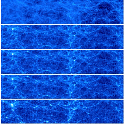
We have performed several simulations using both Gaussian and nongaussian initial conditions. For each Gaussian realization, we construct non-Gaussian realizations using the same Fourier phases, with various , e.g. , , and . We ran simulations from a starting expansion factor until the present time, , using particles in a box of sidelength Mpc. For these parameters, each particle has a mass , so that clusters with masses exceeding are resolved with particles. Since we are interested mainly in the masses and positions of cluster-sized halos, and not their internal structure, we have not used high force resolution: we employ a Plummer softening length of 0.2 times the mean interparticle spacing. We have checked that using higher force resolution ( half as large) does not appreciably change the mass function. All simulations were performed at the Sunnyvale cluster at CITA; depending upon the value of , the simulations completed in 2-3 hours each on typically 8-10 nodes. As a consistency check, we have also run a small number of particle simulations with the same particle mass and force softening as above, but with twice the box size. These larger runs typically completed in 18-20 hours on 64 nodes. In Figure 1, we plot slices through our simulation volume at redshift , and the effects of varying are readily apparent. Large positive accelerates the evolution of overdense regions and retards the evolution of underdense regions, while large negative has precisely the opposite effect.
IV The halo mass function
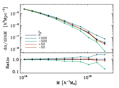
We constructed late-time halo catalogues at redshifts , 0.5, and 0 using the friends-of-friends group finder Davis et al. (1985), with linking length . For Gaussian simulations, the halo mass function constructed this way has been extensively calibrated Jenkins et al. (2001); Warren et al. (2006). Resulting mass functions are plotted in Figure 2.
IV.1 A new fitting formula
Having measured the halo mass function, we next would like to construct a fitting function along the lines of those used for Gaussian simulations Jenkins et al. (2001); Warren et al. (2006). As mentioned above, previous techniques for estimating the nongaussian mass function have been based upon the Press-Schechter Press and Schechter (1974) ansatz. Given that the Press-Schechter mass function fails to match the halo mass function to within an order of magnitude over the mass and redshift ranges of interest to us Warren et al. (2006), and given the lack of any physical basis to the Press-Schechter ansatz Bond et al. (1991); Bond and Myers (1996), we have instead adopted an alternative approach which we describe next.
We start by noting that the halo mass function has been precisely calibrated for Gaussian cosmologies. Consider a Gaussian realization of the density field, which at late times evolves to produce halos with mass function . As we slowly vary away from zero, the structures forming at late times also slowly vary (c.f. Figure 1), producing a different mass spectrum . If we vary slowly enough, we can track the change in mass and position for individual halos: i.e., for each halo of mass for , we can uniquely identify a corresponding halo of mass for , as long as is sufficiently small. Since we know precisely the number of halos as a function of , if we can determine the mapping , we will then have an estimate of the non-Gaussian mass function via
| (11) |
where is the probability distribution that a Gaussian halo of mass maps to a non-Gaussian halo of mass . Note that the probability distribution function need not integrate to unity, in general, since the total number of halos is not conserved: halos can merge or split as is varied.
The next step is to determine the probability distribution , by matching halos between Gaussian and non-Gaussian simulations. We match halos by requiring that matching pairs have significantly overlapping Lagrangian volumes; i.e. by requiring that halos have many particles in common, where particles are labeled by their Lagrangian coordinates in the initial conditions. For each halo in a non-Gaussian run, we loop over the halo’s particles and identify which Gaussian halos own those particles in the run with . The Gaussian halo owning the largest fraction (exceeding 1/3) of the particles is then identified as the match for non-Gaussian halo . Each Gaussian halo can have one, several, or zero matching non-Gaussian halos, depending on . By stacking Gaussian halos of similar mass , we can determine .
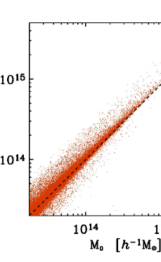
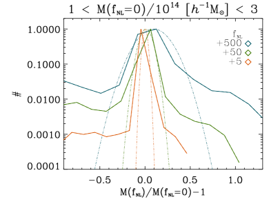
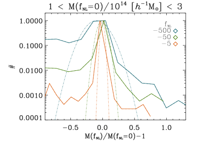
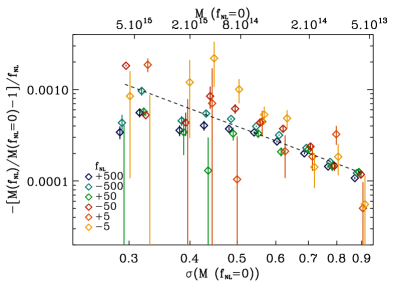
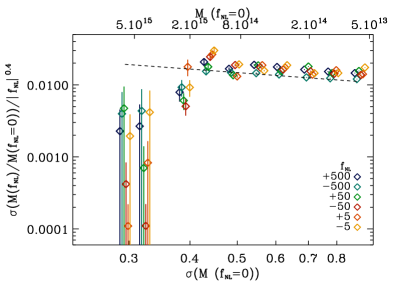
Examples of the probability distribution are shown in Figure 4, and the mean and variance of the PDF are plotted in Figure 5. The behavior of the mean and variance are quite regular, and appear consistent with simple power laws:
| (12) | |||||
| (13) |
where the rms overdensity dispersion is defined as usual by
| (14) |
where we use a top-hat window for , and and are the matter power spectrum and energy density respectively.
Because we desire a simple fitting formula, we assume that we can approximate the PDF as a normalized Gaussian whose mean and variance are given above, even though the PDF shape is quite clearly nongaussian (c.f. Figure 4). As we show below, however, even this crude approximation is sufficient to achieve the precision in the halo mass function provided by standard fitting formulae for Gaussian simulations Lukic et al. (2007). Then Eq. (11), together with which is assumed to be a Gaussian with the mean and variance given in Eqs. (12) and (13), fully specify our fitting function. Essentially, we have written the NG mass function as a convolution of the Gaussian mass function with a Gaussian kernel.
IV.2 Review of previous fitting formulae
Before showing a comparison of the simulated mass function to our proposed fitting formula, we first describe alternative fitting formulae previously suggested in the literature: the Extended Press-Schechter (EPS) formalism Sefusatti et al. (2007), and the model of Matarrese et al. (2000, hereafter MVJ).
IV.2.1 Extended Press-Schechter
The EPS formalism generalizes the widely used Press-Schechter Press and Schechter (1974) model, which posits that the fraction of mass in collapsed objects is equal to twice the fraction of the volume occupied by density peaks exceeding some critical overdensity . (The factor of two arises from the so-called ‘cloud-in-cloud’ problem Bond et al. (1991).) Therefore the collapsed fraction becomes
| (15) | |||||
| (16) |
where the probability distribution that the density smoothed on mass scale equals is simply , the Gaussian distribution with zero mean and unit variance for , with given by Eq. (14). Note that for hierarchical cosmologies where diverges as ; that is, all matter is assumed to be in virialized objects of some mass.
The differential mass function may then be readily computed:
| (17) |
For a Gaussian PDF, the mass enters the right-hand side of this expression only via the lower bound of the integral, , so we immediately obtain
| (18) |
This gives the well-known Press-Schechter mass function.
A class of fitting formulae based on this approach, and loosely called ‘Extended Press-Schechter’ (though apparently unrelated to the work of Refs. Lacey and Cole (1993); Bower (1991)) attempt to generalize this argument using nongaussian PDFs. The most obvious way of making this generalization, i.e. inserting the nongaussian PDF into Eq. (17), faces several immediate difficulties, however. First, the Press-Schechter factor of 2 is no longer valid; rather the cloud-in-cloud correction will depend upon the specific form of nongaussianity. Second, the shape of the PDF now depends upon and so we cannot simply replace the derivative of the integral in Eq. (17) by the integrand. Lastly, and prosaically, the Press-Schechter mass function does not, in fact, fit the halo mass function in N-body simulations well, and so starting from PS is guaranteed to fail in fitting the nongaussian mass function.
The approach adopted by many previous workers (e.g. Sefusatti et al. (2007)) has instead been to assume that, although Press-Schechter cannot be used to derive the Gaussian mass function, it may be used to compute the departure of the mass function from its Gaussian value, i.e.
| (19) |
where is given by Eq. (15). In this approach, the nongaussian mass function is computed by multiplying the Gaussian mass function (not Press-Schechter, but Jenkins et al. (2001) or Warren et al. (2006)) by the above ratio.
The EPS prediction for the halo mass function is therefore given by the derivatives of the PDF tails given in Eq. (19) above. To implement this prescription, we compute the PDF tails directly from the initial conditions of our simulations: at each redshift we are interested in, we integrate the linearly evolved PDF to compute at masses ranging from about to . Then we compute the mean value of averaged over 10 independent N-body simulations. Finally, we fit a cubic spline through the (computed mean of) and differentiate with respect to mass. Evaluation of this formula becomes extremely difficult at high masses, simply because the statistics of peaks at these high masses becomes too noisy.
IV.2.2 MVJ
The MVJ Matarrese et al. (2000) mass function is a further approximation to the EPS model described above. Instead of numerically computing the PDF and its tails for each , it is assumed that the ratio in Eq. (19) may be determined from the skewness of the PDF. The expression for the mass function becomes Grossi et al. (2007)
where
| (21) | |||||
| (22) |
where is th moment of the density field evaluated on the characteristic mass scale , and is the skewness on that mass scale.
The advantage of the MVJ formula is that it does not require specification of the PDF of the density field — however, it does require knowledge of the skewness . In this work, we compute the moments of the density field directly from our simulations at the starting epoch , then scale them with the linear growth function to the desired epoch. We can then evaluate the MVJ expression in Eq. (IV.2.2). Unlike the EPS approach described above, the formula does not become intractable at high masses. On the other hand, MVJ becomes onerously expensive to calculate at low levels of nongaussianity (e.g. ), simply because the scatter in the measured skewness from run to run becomes comparable to that generated by primordial nongaussianity. To see this, note that the scatter in is roughly for samples. Approximating , then for a grid and mass scale of 200 cells, and taking , requiring translates into .
IV.3 Results and comparison to previous work
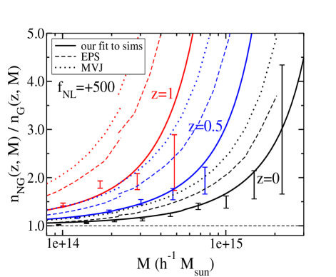
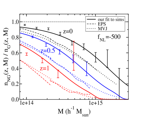
Figure 6 shows the ratios for (left panel) and (right panel). Simulation values are denoted with error bars, colored black (), blue () and red (). To compute the error bars in the ratios, and taking account of the fact that and measurements are correlated, we have adopted the larger error of the two alone (rather than adding them in quadrature), which is the error in () for (). The solid lines denote our fits explained in Sec. III. Dashed lines refer to the EPS results, while the dotted lines represent the MVJ fitting function. The results clearly indicate that, while the EPS and the MVJ functions mutually agree333The agreement between the EPS and MVJ is even better when an alternative expression is used in for , as pointed out Grossi et al. (2007); see their Eq. (4). We have not used this correction in our Fig. 6., they both overestimate the effects of nongaussianity as found by our simulations, at a level typically although dependent upon mass and redshift.
This result appears to disagree with the work of Kang et al. (2007), who find a large discrepancy between EPS/MVJ and their simulations’ mass function, in the sense that their simulations show a much larger effect of nongaussianity than predicted by the EPS type formalism. However, as noted by these authors, their simulations used a rather small number of particles () in a volume nearly 20 smaller than ours, so it is unclear how well they probe the statistics of the rare objects of interest to us. In contrast, Grossi et al. (2007) have found very good agreement between the MVJ formula and their simulations’ results. While our fitting function is in mild disagreement with the MVJ fitting formula, it is unclear whether our simulations are in disagreement with the simulations of Grossi et al. (2007). Their simulations used a somewhat different cosmological model (higher ) than ours, they have plotted cumulative rather than differential mass functions, and of course the error bars in both their plots and ours are considerable.
In summary, we conclude that our simple fitting function appears consistent with the measured mass function from our simulations to within over the entire range of masses and redshifts that we consider. Since this is the level of precision that various N-body codes agree with each other in the mass function Lukic et al. (2007), we have not attempted to achieve better agreement. EPS-like fitting formulae, such as the model of MVJ Matarrese et al. (2000), appear to overestimate the effects of nongaussianity. The level of discrepancy increases with increasing mass and redshift.
V Halo clustering
Beyond one-point statistics like the halo mass function, N-body simulations also allow us to compute higher order statistics like the correlation function or its Fourier transform, the power spectrum. As shown in Sec. A.2, we expect nongaussianity to produce pronounced effects on the halo power spectrum, specifically in the form of scale-dependent halo bias on large scales. This may seem somewhat surprising, due to very general arguments previously given in the literature that galaxy bias is expected to be independent of scale in the linear regime Coles (1993); Fry and Gaztanaga (1993); Scherrer and Weinberg (1998). We can summarize the argument as follows. Suppose that the halo overdensity is some deterministic function of the local matter overdensity, . On large scales, where , we can Taylor expand this function, . Keeping only the lowest order terms and requiring that then gives , which is linear deterministic bias. The key assumption in this argument was locality; i.e. that the halo abundance is determined entirely by the local matter density. N-body simulations with Gaussian initial conditions have confirmed that halo bias tends to a constant on large scales well in the linear regime.
Once we allow for primordial nongaussianity, however, the above argument need not hold. For example, in this paper we have considered NG of the form , and note that the gravitational potential is a nonlocal quantity. Hence the locality-based argument above does not apply for this form of nongaussianity, and our derived scale-dependence of the bias is not surprising. The specific form we have derived is particular to the quadratic, local form of NG that we have assumed, however we expect any NG that couples density modes with potential modes will in general lead to scale-dependent bias. On the other hand, nongaussianity of the form does not lead to scale-dependent bias.
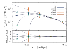
In order to test our prediction for the scale dependence of bias, we have computed halo bias in our N-body simulations by taking the ratio of the matter power spectrum and the halo-matter cross spectrum . We have used the cross spectrum rather than the halo auto spectrum because the former should be less sensitive to shot noise from the small number of halos compared to DM particles. We have checked, however, that using the halo auto-spectra to compute bias gives consistent results as the cross-spectra; i.e. we find no evidence for stochasticity. Examples of the various power spectra and resulting bias factors are plotted in figure Fig. 7.
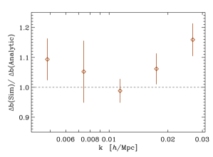
As can be seen, we numerically confirm the form of the predicted scale dependence. Because we focus on the statistics of rare objects, the errors on bias from individual simulations plotted in Fig. 8 is large. We therefore attempt to improve the statistics on the comparison by combining the bias measurements from multiple simulations. Figure 8 plots the average ratio between the bias measured in our simulations and our analytic prediction Eqn. (9), using as predicted from the spherical collapse model Gunn and Gott (1972). In computing the average plotted in this figure, we used a uniform weighting across the different simulations, redshifts, and mass bins. Alternative weightings can shift the results by , so we conservatively estimate the systematic error in our comparison to be 20%. The agreement between our numerical simulation results and our predicted bias scale-dependence, Eqn. (9), is excellent and perhaps surprising. Naively, we might expect a somewhat larger collapse threshold to apply, considering the ellipsoidal rather than spherical nature of the collapse of halos in this mass range Bond and Myers (1996).
VI Cosmological consequences
Having derived fitting formulae for the abundance and clustering of halos in NG models, we now investigate how well upcoming surveys may constrain , and whether NG could possibly affect the constraints derived on other cosmological parameters. We focus on galaxy cluster surveys and redshift surveys. Cluster surveys aim to constrain cosmological parameters, in particular dark energy parameters, by exploiting the exponential sensitivity of the galaxy cluster abundance on cosmology. Similarly, a major goal for upcoming redshift surveys is to constrain dark energy by localizing baryonic acoustic oscillation (BAO) features in the galaxy power spectrum at multiple redshifts. Examples of upcoming surveys include the Atacama Cosmology Telescope444http://wwwphy.princeton.edu/act/, South Pole Telescope555http://spt.uchicago.edu, Dark Energy Survey666http://www.darkenergysurvey.org, WiggleZ777http://astronomy.swin.edu.au/wigglez/WiggleZ/Welcome.html, Planck888http://www.rssd.esa.int/Planck, SuperNova/Acceleration Probe999http://snap.lbl.gov, and the Large Synoptic Survey Telescope101010http://www.lsst.org.
Because primordial nongaussianity affects both the abundance and power spectra of massive halos, both of these types of surveys will be well-suited for constraining NG. On the other hand, potential NG could in principle degrade the expected constraints on dark energy parameters, due to possible degeneracies. We use the Fisher matrix formalism to extract errors on seven cosmological parameters as well as . Our estimates are only illustrative; accurate forecasts for specific surveys will require a more sophisticated analysis.
VI.1 Constraints from :
Galaxy surveys, BAO and ISW
We can (crudely) estimate constraints on parameters derived from measurements of the power spectrum by assuming that bandpowers are measured with errors , where is the power in a band of width centered at wavenumber , is the number density of galaxies, and is the number of independent Fourier modes sampled by the survey, roughly given by Blake et al. (2006). Then the Fisher matrix can be written as
| (23) |
For simplicity, in Eq. (23) we use the linear theory power spectrum and number density corresponding to , and assume an all-sky, volume-limited survey extending to . We integrate over wavenumbers between Mpc and Mpc. The results are insensitive to but depend strongly on . We believe the used here is optimistic but reasonable. At high (small scales), late-time nonlinear evolution can also generate scale-dependent bias Smith et al. (2007a), however the redshift and scale dependence of this effect is quite distinctive from NG and we ignore it here.
We assume that the target galaxies have properties similar to luminous red galaxies (LRGs) Padmanabhan et al. (2007), with comoving number density and bias . Equation (23) then gives estimated errors on of , which compares well with forecasted constraints on nongaussianity for Planck.
Unsurprisingly, we find little degeneracy between and other cosmological parameters, given its distinctive effect on the shape of the power spectrum. Accordingly, there is little reason to believe that BAO determinations of dark energy parameters will be biased by nongaussianity, especially since the scale dependence is small over the wavenumbers of interest for the BAO wiggles. To quantify this effect we determine the acoustic peak position by looking at extrema of the ratio of the power spectra with baryons and the power spectrum with zero baryons Eisenstein and Hu (1999). When multiplying the matter power spectrum with baryons by our scale dependant bias, we find that would shift the first BAO peak at Mpc by 0.4% at , and has a considerably smaller effect at the higher BAO peaks. The magnitude of this effect is comparable to the effect of non-linear corrections to the power spectrum Crocce and Scoccimarro (2007); Smith et al. (2007b), although the NG effect is primarily important on large scales while nonlinearities are most important on small scales. In principle, NG and nonlinearities could conspire to lead to a bias in the dark energy equation of state parameter inferred from BAO observations Crocce and Scoccimarro (2007), and so a careful joint analysis allowing both for NG and nonlinear corrections will be required, which should not be difficult.
Another probe of on large scales is the cross-correlation between cosmic microwave background (CMB) temperature anisotropies and large scale structure, due to the integrated Sachs-Wolfe (ISW) effect Sachs and Wolfe (1967); Crittenden and Turok (1996); Bean and Dore (2004). First detections of the ISW effect from cross-correlations of WMAP with various large scale surveys have been obtained with reported detections at the 2-4 level Boughn and Crittenden (2004); Nolta et al. (2004); Fosalba et al. (2003); Scranton et al. (2003); Fosalba and Gaztañaga (2004); Padmanabhan et al. (2005a); Afshordi et al. (2004); Cabre et al. (2006). A combined analysis yields a detection Scranton et al. (2007), whereas a cosmic variance limited measurement would allow a detection for the currently favored CDM cosmology, and a somewhat more significant detection if the dark energy equation of state parameter is smaller Afshordi (2004); Hu and Scranton (2004). The cross-correlation between large-scale structure and CMB is directly proportional to a weighted projection of the scale-dependant bias. Since the and dependence of our bias is very specific, we do not expect it to be severely degenerate with other parameters affecting the amplitude of the ISW effect (mostly and for a flat universe). We can thus translate the ISW detection level into constraints on . For the sake of simplicity, we assume that the ISW signal comes from and is dominated by the angular multipole , corresponding to a wavenumber Mpc at Afshordi (2004). According to Eq. (9) the current () detections of ISW translate into upper limits on of 123 (61) (1) assuming a bias , as appropriate for LRGs Padmanabhan et al. (2005a). A prospective 7.5 detection would translate into (1). These estimates are clearly very crude, but are likely correct at the order of magnitude level. In comparison, the current limit from CMB bispectrum measurements from WMAP give -54 114 (95% CL) Spergel et al. (2007) whereas Planck is expected to constrain (1 ) Smith and Zaldarriaga (2006b).
In summary, the large-scale galaxy power spectrum appears capable of constraining local NG quite stringently for surveys reaching Gpc scales: . ISW or BAO observations could provide somewhat weaker bounds on , though of course any constraints they can provide would be independent of the CMB bispectrum and therefore worthwhile. Our estimates of forecasted bounds on were rather crude, but given the encouraging results, a more sophisticated treatment for specific survey parameters appears warranted.
VI.2 Constraints from cluster counts
We next consider how well upcoming cluster surveys can constrain by measurements of the cluster mass function . Other forms of nongaussianity may also be constrained by these surveys Sadeh et al. (2007), but we focus on the form. For our fiducial survey parameters, we consider a fixed, redshift-independent lower mass limit of and assume redshift bins of width uniformly distributed between and . We simultaneously vary seven cosmological parameters besides : , the normalization of the primordial power spectrum at ; physical matter and baryon densities and , spectral index , the sum of the neutrino masses , the matter energy density today relative to critical , and the equation of state parameter of dark energy . We assume no mass information (which would improve our parameter constraints) but also no systematic errors (which would degrade the constraints). We further assume 5000 square degrees on the sky, roughly consistent with expectations for the Dark Energy Survey or the South Pole Telescope. The fiducial survey has about 7000 clusters (for cosmology) and about 23,000 for ). We use WMAP3 Spergel et al. (2007) cosmological parameters in determining error forecasts. The mass power spectrum is written as
| (24) |
where is the transfer function adopted from Eisenstein and Hu (1999), and the growth function is computed exactly by integrating the well known second order differential equation for growth (e.g. Eq. (1) in Cooray et al. (2004)).
Following the results of section IV.1, we assume that the mass function may be written as
| (25) |
where the nongaussian correction is computed using either our fitting formula, or EPS for comparison. For a given mass function, the total number of objects in a redshift interval of width and centered at is
| (26) |
where is the total solid angle covered by the survey, is the comoving density of clusters more massive than , and is the comoving volume element. We assume square degrees, roughly consistent with expectations for the Dark Energy Survey or the South Pole Telescope. The fiducial survey has about 7000 clusters (for cosmology) and about 23,000 (for ).
Assuming Poisson statistics, the Fisher information matrix reads Holder et al. (2001); Huterer et al. (2004); Lima and Hu (2004)
| (27) |
where are the 8 cosmological parameters including , is the number of clusters th redshift bin, and the sum runs over the redshift bins extending to maximal redshift 111111Some attention needs to be paid when taking the derivative with respect to , as it is especially with this parameter that the assumption that the likelihood function Gaussian may be violated, leading to results that are weaker or stronger than a full likelihood calculation would reveal. We explore different values of and find convergence at . We also find, however, that the sensitivity to (and also to the normalization ) is slightly higher when () than when (); this is expected as excess of rare objects like galaxy clusters provides more cosmological leverage than their absence. This implies that true constraints on will be slightly asymmetric around our fiducial value of zero; therefore, we make sure to take two-sided derivatives with . For the EPS function, we take the two-sided derivative with (recall we ran sinulations with , and ), and check that the results are similar, if noisier, if is used.. We assume no mass information (which would improve our parameter constraints) but also no systematic errors (which would degrade the constraints).
Lastly, we add a Planck prior on the parameter set, neglecting forecasted constraints on expected from future CMB bispectrum measurements (since we are interested in the sensitivity to NG of cluster counts alone). The full Fisher matrix is given by
| (28) |
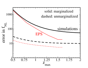
Fig. 9 shows the result of our Fisher matrix estimate, i.e. the forecasted errors on as a function of the maximum extent of the cluster survey, . Black solid and dashed lines show the marginalized and unmarginalized error using our fitting formulae for , while the red lines show the errors using the EPS formalism. The former errors are clearly well behaved, and asymptote at high as expected since cluster abundance rapidly vanishes. On the other hand EPS-produced errors disagree with the simulations by up to a factor of three. Moreover, even though we use the average of the nongaussian PDF tail over 10 simulations, the EPS result becomes noisy at due to poor sampling of the tails. The magnitude of the discrepancy between EPS estimates and our simulations appears similar even for the higher model. As with our estimates from power spectrum constraints, we do not find significant degeneracies between and other cosmological parameters (correlation coefficient ).
Since we find a weaker effect on cluster abundance than previous formulae like EPS or MVJ, this implies that constraints found by Sefusatti et al. (2007), who performed a similar Fisher matrix estimate but with somewhat different assumptions, will be weaker once the NG sensitivity is calibrated off simulations. Direct quantitative comparison to two other relevant papers, Kang et al. (2007) and Grossi et al. (2007), is however difficult since these authors do not compute cosmological parameter error estimates.
VII Discussion
We have quantified the effects of primordial nongaussianity on the abundance and power spectra of massive halos. Our two principal results are as follows.
First, we have provided a new fitting formula for the halo mass function. The formula is based on matching halos in Gaussian and non-Gaussian simulations: for the corresponding halos are more massive than in the Gaussian case, and vice versa. The formula is consistent with the measured mass function from our simulations to within over the entire range of masses and redshifts that we consider. Being essentially a convolution of the Gaussian mass function and a Gaussian kernel (Eqs. (11)-(13)), the formula is also easy to use and does not require estimating the extreme tails of the nongaussian PDF of the density field. Our results also indicate that previous work based on Extended Press-Schechter type formulae overestimated the effects of nongaussianity on the abundance of halos by a factor of over the relevant mass scales.
Secondly, we showed both analytically and numerically that nongaussianity (in the model) leads to strong scale dependence of the bias of dark matter halos. We find remarkably good agreement between our analytic expression and our numerical results. Measurement of the power spectrum of biased objects therefore provides a new avenue to detect and measure nongaussianity. While cluster counts can constrain NG at a level comparable to existing CMB constraints, , we found that future large-scale redshift surveys can potentially do much better, roughly . We do not find significant degeneracies between and dark energy parameters in our Fisher matrix calculations, either for mass function measurements or power spectrum measurements. More precise estimates will require considerably more sophisticated treatments than we have attempted in our illustrative examples above.
We close this paper by considering, in light of our findings, the optimal methods for constraining NG of the form. Measurements of the power spectrum would appear the most promising; observations of high redshift, highly clustered objects on large scales would allow the strongest constraints on the scale-dependent bias signature of . Fortunately, upcoming BAO surveys will likely provide the necessary observations of, e.g. luminous red galaxies (LRGs). Photometric surveys may also be useful in this regard. Since the effects of NG are most pronounced on large scales, rather than small scales, precise spectroscopic redshifts may not be necessary. Photometric redshifts with errors of order have already been achieved for LRGs and for optically selected groups and clusters with prominent red sequences Padmanabhan et al. (2005b); Ilbert et al. (2006); Yee et al. (2007). At , this corresponds to roughly 100 Mpc comoving, fairly small compared to the Gpc scales where NG becomes most important. Since photometric surveys can cover wider areas more deeply than spectroscopic surveys, they may turn out to provide tighter bounds.
Besides their abundance and clustering, the internal properties of massive halos may also be sensitive to nongaussianity. For instance, the concentrations and substructure content of massive halos have been found to depend upon primordial NG Avila-Reese et al. (2003). Our simulations lacked sufficient force resolution to explore this in detail, but we note in passing that multiple groups find a tension between observations of massive lensing clusters and theoretical predictions for Gaussian perturbations Gladders et al. (2003); Dalal et al. (2004); Hennawi et al. (2007); Broadhurst and Barkana (2008).
Another intriguing possibility for probing primordial NG is to use statistics of the largest voids in the universe. Just as the abundance and clustering of high density peaks are affected by nongaussianity, so are the same properties for deep voids (albeit with an opposite sign, c.f. Fig. 1). In a sense, because voids are not as nonlinear as overdense regions, their properties are more easily related to the initial Lagrangian underdensities whose statistics are straightforward to compute. Voids may be detected at high redshift as a deficit of Lyman- forest absorption features in QSO spectra. The Sloan Digital Sky Survey (SDSS) has already measured spectra for high redshift QSO’s over a roughly 8000 deg2 area, corresponding to a volume of McDonald et al. (2006). Each QSO spectrum typically probes Mpc, and the typical transverse separation between QSO sightlines in SDSS is Mpc, (P. McDonald, priv. comm.) so measurements of the clustering of Mpc-sized voids on Gpc scales may already be feasible.
Finally, we note that our conclusions are based on simulations implementing a very specific type of local primordial nongaussianity quantified by the parameter. The validity of our conclusions in the context of other type of primordial nongaussianity is the subject of ongoing studies.
Acknowledgments
We are grateful to the organisers and participants of the “Life beyond the Gaussian” workshop held at KICP (Chicago, June 2007) where a preliminary version of this work was presented and discussed. We thank Xuelei Chen and the National Astronomical Observatories of the Chinese Academy of Sciences in Beijing where a part of this work was completed. Finally we thank Niayesh Afshordi, Neil Barnaby, Wayne Hu, Lam Hui, Nikhil Padmanabhan, Uros Seljak, Robert Smith, and Emiliano Sefusatti for useful conversations, Wayne Hu for providing the CMB Fisher matrix, and Pat McDonald for discussions of the Lyman- forest. All simulations were performed on CITA’s Sunnyvale cluster, funded by the Canada Foundation for Innovation and the Ontario Research Fund for Research Infrastructure. This work was supported by the Canadian Institute for Theoretical Astrophysics (CITA) and the Natural Sciences and Engineering Research Council of Canada (NSERC).
*
Appendix A The abundance and clustering of high peaks
In this appendix we derive analytic expressions for the abundance and clustering of regions above the spherical collapse threshold . We first review previous results derived for Gaussian statistics, and then show how they are modified by nongaussianity.
A.1 Review of Gaussian results
We begin by identifying massive halos at late times with high peaks in the initial density distribution . Note that we work entirely in early-time, Lagrangian coordinates in this section rather than late-time, Eulerian coordinates. Earlier work Press and Schechter (1974); Kaiser (1984); Bardeen et al. (1986); Bond et al. (1991) has shown that the abundance of peaks above threshold reasonably describes (at the order-of-magnitude level) the statistics of halos forming at subsequent times. We briefly review some of these previous results, as the methods will be used in our analysis.
Following the Press and Schechter (1974) ansatz, we smooth the density field and assume that density peaks with produce halos. The density smoothed on scale is given by
| (29) |
where is some smoothing window, e.g. top-hat or Gaussian. Assuming that the Fourier modes are Gaussian distributed with power spectrum , then also has a Gaussian distribution, with variance
| (30) |
The probability for a given randomly selected region to exceed the threshold is then simply the integral of the Gaussian probability distribution,
| (31) | |||||
where , and similarly .
The same power spectrum describing the density variance also gives the matter correlation function , and, following an elegant argument by Kaiser (1984), can also be used to determine the correlation function of rare peaks. Let us compute the probability that two randomly selected regions separated by distance are both above threshold. Again, this is simply an integral over the (joint) Gaussian distribution:
| (32) |
where , the covariance matrix is given by
| (33) |
and the matter correlation function is given by
| (34) |
Rescaling the ’s by their variance, this becomes
| (35) |
where
| (36) |
and we follow the notation of BBKS Bardeen et al. (1986) in writing the normalized correlation function as ; note that .
To evaluate the integral in Eq. (35), we change coordinates to variables that are uncorrelated. Using the Cholesky decomposition of the covariance matrix , we write for new variables . Next, we rotate coordinates to bring the point along the axis. Then the integral becomes
| (37) | |||||
where the Heaviside function accounts for the two integration bounds. Since , we can write this as
| (38) | |||||
where , and . We could easily evaluate the integral for in terms of the error function, but the resulting integral over would then not be analytic. However, we can derive an approximate solution in the limit . For integrals of the form
| (39) |
we can construct an asymptotic series by repeated partial integrations :
| (40) |
In our case, and . Therefore, in the limit , we obtain
| (41) | |||||
Comparing this expression to the probability for a single peak to be above threshold then gives the peak-peak correlation function , which in the limit , becomes
| (42) | |||||
and therefore the (Lagrangian) bias becomes
| (43) |
A.2 Nongaussianity
Our discussion so far has merely reviewed previous results for Gaussian fluctuations; we now turn to nongaussian fluctuations. As noted above, we focus on NG of the form
| (44) |
We adopt the approximation of §II that the heights of rare peaks are modified by NG as , where in this appendix we adopt the notation that refers to the primordial potential. At late times, decays as the growth suppression factor .
Let us first consider the one-point distribution of peaks above threshold, . We express this as an integral over Gaussian variables and ; the integration bound then becomes , and using the fact that typically , we have . The probability for to exceed threshold then is
| (45) | |||||
where , , , and . We write the off-diagonal part of the normalized covariance matrix as , where the cross-correlation coefficient is not to be confused with the peak-peak separation appearing above and below. By a coordinate transformation, we can orient the integration bound along a single axis. Changing coordinates from to , and noting that the variance of is , we can integrate out to obtain
| (46) |
where . The effect of NG on the peak abundance is therefore simply to rescale the threshold density by a mass- and redshift-dependent factor.
Next, we turn to the peak-peak correlation function. As in the Gaussian case, we write the probability for two points both to be above threshold as
| (47) | |||||
where , and the notation is otherwise the same as above. We write the off-diagonal parts of the normalized covariance matrix as , , , and . As above, we change variables from to to align the integration bounds along the density coordinate axes. This allows us to integrate out the two potential variables, leaving behind a 2-D integral. Rescaling the remaining two variables by their (identical) variance and again writing , brings the integral to the form
| (48) |
where the off-diagonal component of is given by
| (49) |
The form of equation (48) is identical to Eq. (35), with and . So we can immediately write down the approximate solution,
| (50) |
Comparing with the single-peak probability, we obtain the peak-peak correlation function, in the limit , :
| (51) |
which to lowest order in becomes
| (52) | |||||
where was the Lagrangian bias obtained for Gaussian peaks, c.f. Eq. (43). Note that in going from the first line to the second, we neglect relative to since is smaller than by a factor scaling like , where is the smoothing scale of the peak and is the peak-peak separation.
The peak-peak correlation function is now no longer simply proportional to the matter correlation function, implying that the peak bias is not independent of scale. Fourier transforming this expression gives the peak power spectrum,
| (53) |
which gives a scale-dependent change in the bias due to NG of
| (54) | |||||
where we have used the relation between the potential-density cross-spectrum and the matter power spectrum , arising from the Poisson equation. The total Lagrangian bias is then .
References
- Maldacena (2003) J. Maldacena, Journal of High Energy Physics 5, 13 (2003), eprint arXiv:astro-ph/0210603.
- Acquaviva et al. (2003) V. Acquaviva, N. Bartolo, S. Matarrese, and A. Riotto, Nucl. Phys. B667, 119 (2003), eprint astro-ph/0209156.
- Creminelli (2003) P. Creminelli, JCAP 0310, 003 (2003), eprint astro-ph/0306122.
- Lyth and Rodriguez (2005a) D. H. Lyth and Y. Rodriguez, Phys. Rev. Lett. 95, 121302 (2005a), eprint astro-ph/0504045.
- Seery and Lidsey (2005) D. Seery and J. E. Lidsey, JCAP 0506, 003 (2005), eprint astro-ph/0503692.
- Spergel et al. (2007) D. N. Spergel, R. Bean, O. Doré, M. R. Nolta, C. L. Bennett, J. Dunkley, G. Hinshaw, N. Jarosik, E. Komatsu, L. Page, et al., Astrophys. J. Supp. Ser. 170, 377 (2007), eprint arXiv:astro-ph/0603449.
- Creminelli et al. (2007a) P. Creminelli, L. Senatore, M. Zaldarriaga, and M. Tegmark, JCAP 0703, 005 (2007a), eprint astro-ph/0610600.
- Arkani-Hamed et al. (2004) N. Arkani-Hamed, P. Creminelli, S. Mukohyama, and M. Zaldarriaga, JCAP 0404, 001 (2004), eprint hep-th/0312100.
- Bartolo et al. (2004a) N. Bartolo, S. Matarrese, and A. Riotto, Phys. Rev. D69, 043503 (2004a), eprint hep-ph/0309033.
- Lyth and Rodriguez (2005b) D. H. Lyth and Y. Rodriguez, Phys. Rev. D71, 123508 (2005b), eprint astro-ph/0502578.
- Rigopoulos et al. (2006) G. I. Rigopoulos, E. P. S. Shellard, and B. J. W. van Tent, Phys. Rev. D73, 083522 (2006), eprint astro-ph/0506704.
- Allen et al. (2006) L. E. Allen, S. Gupta, and D. Wands, JCAP 0601, 006 (2006), eprint astro-ph/0509719.
- Chen (2005) X. Chen, Phys. Rev. D72, 123518 (2005), eprint astro-ph/0507053.
- Barnaby and Cline (2006) N. Barnaby and J. M. Cline, Phys. Rev. D73, 106012 (2006), eprint astro-ph/0601481.
- Barnaby and Cline (2007a) N. Barnaby and J. M. Cline, Phys. Rev. D75, 086004 (2007a), eprint astro-ph/0611750.
- Barnaby and Cline (2007b) N. Barnaby and J. M. Cline (2007b), eprint arXiv:0704.3426 [hep-th].
- Sasaki et al. (2006) M. Sasaki, J. Valiviita, and D. Wands, Phys. Rev. D74, 103003 (2006), eprint astro-ph/0607627.
- Chen et al. (2007a) X. Chen, M.-x. Huang, S. Kachru, and G. Shiu, JCAP 0701, 002 (2007a), eprint hep-th/0605045.
- Chen et al. (2007b) X. Chen, R. Easther, and E. A. Lim, JCAP 0706, 023 (2007b), eprint astro-ph/0611645.
- Battefeld and Easther (2007) T. Battefeld and R. Easther, JCAP 0703, 020 (2007), eprint astro-ph/0610296.
- Assadullahi et al. (2007) H. Assadullahi, J. Valiviita, and D. Wands (2007), eprint arXiv:0708.0223 [hep-ph].
- Battefeld and Battefeld (2007) D. Battefeld and T. Battefeld, JCAP 0705, 012 (2007), eprint hep-th/0703012.
- Bean et al. (2007) R. Bean, S. E. Shandera, S. H. Henry Tye, and J. Xu, JCAP 0705, 004 (2007), eprint hep-th/0702107.
- Bartolo et al. (2004b) N. Bartolo, E. Komatsu, S. Matarrese, and A. Riotto, Phys. Rept. 402, 103 (2004b), eprint astro-ph/0406398.
- Babich (2005) D. Babich, Phys. Rev. D72, 043003 (2005), eprint astro-ph/0503375.
- Babich et al. (2004) D. Babich, P. Creminelli, and M. Zaldarriaga, JCAP 0408, 009 (2004), eprint astro-ph/0405356.
- Creminelli et al. (2007b) P. Creminelli, L. Senatore, and M. Zaldarriaga, JCAP 0703, 019 (2007b), eprint astro-ph/0606001.
- Smith and Zaldarriaga (2006a) K. M. Smith and M. Zaldarriaga (2006a), eprint astro-ph/0612571.
- Fergusson and Shellard (2006) J. R. Fergusson and E. P. S. Shellard (2006), eprint astro-ph/0612713.
- Falk et al. (1993) T. Falk, R. Rangarajan, and M. Srednicki, Astrophys. J. 403, L1 (1993), eprint astro-ph/9208001.
- Luo and Schramm (1993) X.-c. Luo and D. N. Schramm, Phys. Rev. Lett. 71, 1124 (1993), eprint astro-ph/9305009.
- Gangui et al. (1994) A. Gangui, F. Lucchin, S. Matarrese, and S. Mollerach, Astrophys. J. 430, 447 (1994), eprint astro-ph/9312033.
- Wang and Kamionkowski (2000) L.-M. Wang and M. Kamionkowski, Phys. Rev. D61, 063504 (2000), eprint astro-ph/9907431.
- Verde et al. (2001) L. Verde, R. Jimenez, M. Kamionkowski, and S. Matarrese, Mon. Not. Roy. Astron. Soc. 325, 412 (2001), eprint astro-ph/0011180.
- Scoccimarro et al. (2004) R. Scoccimarro, E. Sefusatti, and M. Zaldarriaga, Phys. Rev. D69, 103513 (2004), eprint astro-ph/0312286.
- Sefusatti and Komatsu (2007) E. Sefusatti and E. Komatsu (2007), eprint arXiv:0705.0343 [astro-ph].
- Lucchin and Matarrese (1988) F. Lucchin and S. Matarrese, Astrophys. J. 330, 535 (1988).
- Robinson and Baker (1999) J. Robinson and J. E. Baker (1999), eprint astro-ph/9905098.
- Benson et al. (2002) A. J. Benson, C. Reichardt, and M. Kamionkowski, Mon. Not. Roy. Astron. Soc. 331, 71 (2002), eprint astro-ph/0110299.
- Matarrese et al. (2000) S. Matarrese, L. Verde, and R. Jimenez, Astrophys. J. 541, 10 (2000), eprint astro-ph/0001366.
- Komatsu et al. (2003) E. Komatsu et al. (WMAP), Astrophys. J. Suppl. 148, 119 (2003), eprint astro-ph/0302223.
- Verde et al. (2001) L. Verde, M. Kamionkowski, J. J. Mohr, and A. J. Benson, Mon. Not. R. Astron. Soc. 321, L7 (2001), eprint arXiv:astro-ph/0007426.
- Rozo et al. (2007) E. Rozo, R. H. Wechsler, B. P. Koester, T. A. McKay, A. E. Evrard, D. Johnston, E. S. Sheldon, J. Annis, and J. A. Frieman, ArXiv Astrophysics e-prints (2007), eprint astro-ph/0703571.
- Koester et al. (2007) B. Koester et al. (SDSS), Astrophys. J. 660, 239 (2007), eprint astro-ph/0701265.
- Eke et al. (2004) V. R. Eke et al. (The 2dFGRS Team), Mon. Not. Roy. Astron. Soc. 348, 866 (2004), eprint astro-ph/0402567.
- Yee et al. (2007) H. K. C. Yee et al. (RCS-2) (2007), eprint astro-ph/0701839.
- Willis et al. (2005) J. P. Willis et al., Mon. Not. Roy. Astron. Soc. 363, 675 (2005), eprint astro-ph/0508003.
- Valtchanov et al. (2004) I. Valtchanov et al., Astron. Astrophys. 423, 75 (2004), eprint astro-ph/0305192.
- Haiman et al. (2001) Z. Haiman, J. J. Mohr, and G. P. Holder, Astrophys. J. 553, 545 (2001), eprint arXiv:astro-ph/0002336.
- Majumdar and Mohr (2003) S. Majumdar and J. J. Mohr, Astrophys. J. 585, 603 (2003), eprint astro-ph/0208002.
- Wang et al. (2004) S. Wang, J. Khoury, Z. Haiman, and M. May, Phys. Rev. D70, 123008 (2004), eprint astro-ph/0406331.
- Battye and Weller (2005) R. A. Battye and J. Weller, Mon. Not. Roy. Astron. Soc. 362, 171 (2005), eprint astro-ph/0410392.
- Lima and Hu (2005) M. Lima and W. Hu, Phys. Rev. D72, 043006 (2005), eprint astro-ph/0503363.
- Marian and Bernstein (2006) L. Marian and G. M. Bernstein, Phys. Rev. D73, 123525 (2006), eprint astro-ph/0605746.
- Takada and Bridle (2007) M. Takada and S. Bridle (2007), eprint arXiv:0705.0163 [astro-ph].
- Robinson and Baker (2000) J. Robinson and J. E. Baker, Mon. Not. R. Astron. Soc. 311, 781 (2000), eprint arXiv:astro-ph/9905098.
- Robinson et al. (2000) J. Robinson, E. Gawiser, and J. Silk, Astrophys. J. 532, 1 (2000), eprint arXiv:astro-ph/9906156.
- Matarrese et al. (2000) S. Matarrese, L. Verde, and R. Jimenez, Astrophys. J. 541, 10 (2000), eprint arXiv:astro-ph/0001366.
- Press and Schechter (1974) W. H. Press and P. Schechter, Astrophys. J. 187, 425 (1974).
- Kang et al. (2007) X. Kang, P. Norberg, and J. Silk, Mon. Not. R. Astron. Soc. 376, 343 (2007), eprint arXiv:astro-ph/0701131.
- Grossi et al. (2007) M. Grossi, K. Dolag, E. Branchini, S. Matarrese, and L. Moscardini, ArXiv e-prints 707 (2007), eprint 0707.2516.
- Komatsu and Spergel (2001) E. Komatsu and D. N. Spergel, Phys. Rev. D 63, 063002 (2001), eprint arXiv:astro-ph/0005036.
- Shirokov and Bertschinger (2005) A. Shirokov and E. Bertschinger, ArXiv Astrophysics e-prints (2005), eprint astro-ph/0505087.
- Shirokov (2005) A. V. Shirokov, Ph.D. thesis, Massachusetts Institute of Technology, Cambridge MA (2005).
- Padmanabhan (1993) T. Padmanabhan, Structure formation in the universe (Cambridge ; New York : Cambridge University Press, 1993., 1993).
- Warren et al. (2006) M. S. Warren, K. Abazajian, D. E. Holz, and L. Teodoro, Astrophys. J. 646, 881 (2006), eprint arXiv:astro-ph/0506395.
- Davis et al. (1985) M. Davis, G. Efstathiou, C. S. Frenk, and S. D. M. White, Astrophys. J. 292, 371 (1985).
- Jenkins et al. (2001) A. Jenkins, C. S. Frenk, S. D. M. White, J. M. Colberg, S. Cole, A. E. Evrard, H. M. P. Couchman, and N. Yoshida, Mon. Not. R. Astron. Soc. 321, 372 (2001), eprint arXiv:astro-ph/0005260.
- Bond et al. (1991) J. R. Bond, S. Cole, G. Efstathiou, and N. Kaiser, Astrophys. J. 379, 440 (1991).
- Bond and Myers (1996) J. R. Bond and S. T. Myers, Astrophys. J. Supp. Ser. 103, 1 (1996).
- Lukic et al. (2007) Z. Lukic, K. Heitmann, S. Habib, S. Bashinsky, and P. M. Ricker, ArXiv Astrophysics e-prints (2007), eprint astro-ph/0702360.
- Sefusatti et al. (2007) E. Sefusatti, C. Vale, K. Kadota, and J. Frieman, Astrophys. J. 658, 669 (2007), eprint arXiv:astro-ph/0609124.
- Lacey and Cole (1993) C. Lacey and S. Cole, Mon. Not. R. Astron. Soc. 262, 627 (1993).
- Bower (1991) R. G. Bower, Mon. Not. R. Astron. Soc. 248, 332 (1991).
- Coles (1993) P. Coles, Mon. Not. R. Astron. Soc. 262, 1065 (1993).
- Fry and Gaztanaga (1993) J. N. Fry and E. Gaztanaga, Astrophys. J. 413, 447 (1993), eprint arXiv:astro-ph/9302009.
- Scherrer and Weinberg (1998) R. J. Scherrer and D. H. Weinberg, Astrophys. J. 504, 607 (1998), eprint arXiv:astro-ph/9712192.
- Smith et al. (2007a) R. E. Smith, R. Scoccimarro, and R. K. Sheth, Phys. Rev. D 75, 063512 (2007a), eprint arXiv:astro-ph/0609547.
- Gunn and Gott (1972) J. E. Gunn and J. R. I. Gott, Astrophys. J. 176, 1 (1972).
- Blake et al. (2006) C. Blake, D. Parkinson, B. Bassett, K. Glazebrook, M. Kunz, and R. C. Nichol, Mon. Not. R. Astron. Soc. 365, 255 (2006), eprint arXiv:astro-ph/0510239.
- Padmanabhan et al. (2007) N. Padmanabhan, D. J. Schlegel, U. Seljak, A. Makarov, N. A. Bahcall, M. R. Blanton, J. Brinkmann, D. J. Eisenstein, D. P. Finkbeiner, J. E. Gunn, et al., Mon. Not. R. Astron. Soc. 378, 852 (2007), eprint arXiv:astro-ph/0605302.
- Eisenstein and Hu (1999) D. J. Eisenstein and W. Hu, Astrophys. J. 511, 5 (1999), eprint arXiv:astro-ph/9710252.
- Crocce and Scoccimarro (2007) M. Crocce and R. Scoccimarro (2007), eprint arXiv:0704.2783 [astro-ph].
- Smith et al. (2007b) R. E. Smith, R. Scoccimarro, and R. K. Sheth, ArXiv Astrophysics e-prints (2007b), eprint astro-ph/0703620.
- Sachs and Wolfe (1967) R. K. Sachs and A. M. Wolfe, Astrophys. J. 147, 73 (1967).
- Crittenden and Turok (1996) R. G. Crittenden and N. Turok, Phys. Rev. Lett. 76, 575 (1996), eprint astro-ph/9510072.
- Bean and Dore (2004) R. Bean and O. Dore, Phys. Rev. D69, 083503 (2004), eprint astro-ph/0307100.
- Boughn and Crittenden (2004) S. Boughn and R. Crittenden, Nature (London) 427, 45 (2004).
- Nolta et al. (2004) M. R. Nolta et al. , Astrophys. J. 608, 10 (2004), eprint astro-ph/0305097.
- Fosalba et al. (2003) P. Fosalba et al. , Astrophys. J. Lett. 597, L89 (2003).
- Scranton et al. (2003) R. Scranton et al. , ArXiv Astrophysics e-prints (2003), eprint astro-ph/0307335.
- Fosalba and Gaztañaga (2004) P. Fosalba and E. Gaztañaga, Mon. Not. R. Astron. Soc. 350, L37 (2004), eprint astro-ph/0305468.
- Padmanabhan et al. (2005a) N. Padmanabhan et al., Phys. Rev. D72, 043525 (2005a), eprint astro-ph/0410360.
- Afshordi et al. (2004) N. Afshordi, Y.-S. Loh, and M. A. Strauss, Phys. Rev. D 69, 083524 (2004), eprint astro-ph/0308260.
- Cabre et al. (2006) A. Cabre et al. , ArXiv Astrophysics e-prints (2006), eprint astro-ph/0603690.
- Scranton et al. (2007) R. Scranton et al. , in preparation (2007).
- Afshordi (2004) N. Afshordi, Phys. Rev. D70, 083536 (2004), eprint astro-ph/0401166.
- Hu and Scranton (2004) W. Hu and R. Scranton, Phys. Rev. D70, 123002 (2004), eprint astro-ph/0408456.
- Smith and Zaldarriaga (2006b) K. M. Smith and M. Zaldarriaga (2006b), eprint astro-ph/0612571.
- Sadeh et al. (2007) S. Sadeh, Y. Rephaeli, and J. Silk, Mon. Not. R. Astron. Soc. 380, 637 (2007), eprint arXiv:0706.1340.
- Cooray et al. (2004) A. Cooray, D. Huterer, and D. Baumann, Phys. Rev. D69, 027301 (2004), eprint astro-ph/0304268.
- Holder et al. (2001) G. Holder, Z. Haiman, and J. Mohr, Astrophys. J. 560, L111 (2001), eprint astro-ph/0105396.
- Huterer et al. (2004) D. Huterer, A. Kim, L. M. Krauss, and T. Broderick, Astrophys. J. 615, 595 (2004), eprint astro-ph/0402002.
- Lima and Hu (2004) M. Lima and W. Hu, Phys. Rev. D70, 043504 (2004), eprint astro-ph/0401559.
- Padmanabhan et al. (2005b) N. Padmanabhan et al. (SDSS), Mon. Not. Roy. Astron. Soc. 359, 237 (2005b), eprint astro-ph/0407594.
- Ilbert et al. (2006) O. Ilbert et al. (2006), eprint astro-ph/0603217.
- Avila-Reese et al. (2003) V. Avila-Reese, P. Colín, G. Piccinelli, and C. Firmani, Astrophys. J. 598, 36 (2003), eprint arXiv:astro-ph/0306293.
- Gladders et al. (2003) M. D. Gladders, H. Hoekstra, H. K. C. Yee, P. B. Hall, and L. F. Barrientos, Astrophys. J. 593, 48 (2003), eprint arXiv:astro-ph/0303341.
- Dalal et al. (2004) N. Dalal, G. Holder, and J. F. Hennawi, Astrophys. J. 609, 50 (2004), eprint arXiv:astro-ph/0310306.
- Hennawi et al. (2007) J. F. Hennawi, N. Dalal, P. Bode, and J. P. Ostriker, Astrophys. J. 654, 714 (2007), eprint arXiv:astro-ph/0506171.
- Broadhurst and Barkana (2008) T. Broadhurst and R. Barkana, ArXiv e-prints 801 (2008), eprint 0801.1875.
- McDonald et al. (2006) P. McDonald, U. Seljak, S. Burles, D. J. Schlegel, D. H. Weinberg, R. Cen, D. Shih, J. Schaye, D. P. Schneider, N. A. Bahcall, et al., Astrophys. J. Supp. Ser. 163, 80 (2006), eprint arXiv:astro-ph/0405013.
- Kaiser (1984) N. Kaiser, Astrophys. J. Lett. 284, L9 (1984).
- Bardeen et al. (1986) J. M. Bardeen, J. R. Bond, N. Kaiser, and A. . S. Szalay, Astrophys. J. 304, 15 (1986).