A quick search method for audio signals based on a piecewise linear representation of feature trajectories

Abstract

This paper presents a new method for a quick similarity-based search through long unlabeled audio streams to detect and locate audio clips provided by users. The method involves feature-dimension reduction based on a piecewise linear representation of a sequential feature trajectory extracted from a long audio stream. Two techniques enable us to obtain a piecewise linear representation: the dynamic segmentation of feature trajectories and the segment-based Karhunen-Lóeve (KL) transform. The proposed search method guarantees the same search results as the search method without the proposed feature-dimension reduction method in principle. Experiment results indicate significant improvements in search speed. For example the proposed method reduced the total search time to approximately 1/12 that of previous methods and detected queries in approximately 0.3 seconds from a 200-hour audio database.

I Introduction

This paper presents a method for searching quickly through unlabeled audio signal archives (termed stored signals) to detect and locate given audio clips (termed query signals) based on signal similarities.

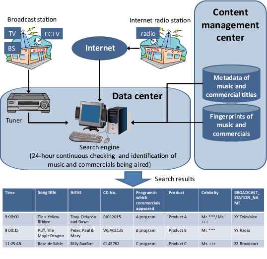
Many studies related to audio retrieval have dealt with content-based approaches such as audio content classification [1, 2], speech recognition [3], and music transcription [3, 4]. Therefore, these studies mainly focused on associating audio signals with their meanings. In contrast, this study aims at achieving a similarity-based search or more specifically fingerprint identification, which constitutes a search of and retrieval from unlabeled audio archives based only on a signal similarity measure. That is, our objective is signal matching, not the association of signals with their semantics. Although the range of applications for a similarity-based search may seem narrow compared with content-based approaches, this is not actually the case. The applications include the detection and statistical analysis of broadcast music and commercial spots, and the content identification, detection and copyright management of pirated copies of music clips. Fig. 1 represents one of the most representative examples of such applications, which has already been put to practical use. This system automatically checks and identifies broadcast music clips or commercial spots to provide copyright information or other detailed information about the music or the spots.

Figure 1: Automatic monitoring system of broadcast content via music content identification.

In audio fingerprinting applications, the query and stored signals cannot be assumed to be exactly the same even in the corresponding sections of the same sound, owing to, for example, compression, transmission and irrelevant noises. Meanwhile, for the applications to be practically viable, the features should be compact and the feature analysis should be computationally efficient. For this purpose, several feature extraction methods have been developed to attain the above objectives. Cano et al. [5] modeled music segments as sequences of sound classes estimated via unsupervised clustering and hidden Markov models (HMMs). Burges et al. [6] employed several layers of Karhunen-Lóeve (KL) transforms, which reduced the local statistical redundancy of features with respect to time, and took account of robustness to shifting and pitching. Oostveen et al. [7] represented each frame of a video clip as a binary map and used the binary map sequence as a feature. This feature is robust to global changes in luminance and contrast variations. Haitsma et al. [8] and Kurozumi et al. [9] each employed a similar approach in the context of audio fingerprinting. Wang [10] developed a feature-point-based approach to improve the robustness. Our previous approach called the Time-series Active Search (TAS) method [11] introduced a histogram as a compact and noise-robust fingerprint, which models the empirical distribution of feature vectors in a segment. Histograms are sufficiently robust for monitoring broadcast music or detecting pirated copies. Another novelty of this approach is its effectiveness in accelerating the search. Adjacent histograms extracted from sliding audio segments are strongly correlated with each other. Therefore, unnecessary matching calculations are avoided by exploiting the algebraic properties of histograms.

Another important research issue regarding similarity-based approaches involves finding a way to speed up the search. Multi-dimensional indexing methods [12, 13] have frequently been used for accelerating searches. However, when feature vectors are high-dimensional, as they are typically with multimedia signals, the efficiency of the existing indexing methods deteriorates significantly [14, 15]. This is why search methods based on linear scans such as the TAS method are often employed for searches with high-dimensional features. However, methods based solely on linear scans may not be appropriate for managing large-scale signal archives, and therefore dimension reduction should be introduced to mitigate this effect.

To this end, this paper presents a quick and accurate audio search method that uses dimensionality reduction of histogram features. The method involves a piecewise linear representation of histogram sequences by utilizing the continuity and local correlation of the histogram sequences. A piecewise linear representation would be feasible for the TAS framework since the histogram sequences form trajectories in multi-dimensional spaces. By incorporating our method into the TAS framework, we significantly increase the search speed while guaranteeing the same search results as the TAS method. We introduce the following two techniques to obtain a piecewise representation: the dynamic segmentation of the feature trajectories and the segment-based KL transform.

The segment-based KL transform involves the dimensionality reduction of divided histogram sequences (called segments) by KL transform. We take advantage of the continuity and local correlation of feature sequences extracted from audio signals. Therefore, we expect to obtain a linear representation with few approximation errors and low computational cost. The segment-based KL transform consists of the following three components: The basic component of this technique reduces the dimensionality of histogram features. The second component that utilizes residuals between original histogram features and features after dimension reduction greatly reduces the required number of histogram comparisons. Feature sampling is introduced as the third component. This not only saves the storage space but also contributes to accelerating the search.

Dynamic segmentation refers to the division of histogram sequences into segments of various lengths to achieve the greatest possible reduction in the average dimensionality of the histogram features. One of the biggest problems in dynamic segmentation is that finding the optimal set of partitions that minimizes the average dimensionality requires a substantial calculation. The computational time must be no more than that needed for capturing audio signals from the viewpoint of practical applicability. To reduce the calculation cost, our technique addresses the quick suboptimal partitioning of the histogram trajectories, which consists of local optimization to avoid recursive calculations and the coarse-to-fine detection of segment boundaries.

This paper is organized as follows: Section II introduces the notations and definitions necessary for the subsequent explanations. Section III explains the TAS method upon which our method is founded. Section IV outlines the proposed search method. Section V discusses a dimensionality reduction technique with the segment-based KL transform. Section VI details dynamic segmentation. Section VII presents experimental results related to the search speed and shows the advantages of the proposed method. Section VIII further discusses the advantages and shortcomings of the proposed method as well as providing additional experimental results. Section IX concludes the paper.

II Preliminaries

Let $\mathcal{N}$ be the set of all non-negative numbers, $\mathcal{R}$ be the set of all real numbers, and $\mathcal{N}^{n}$ be a $n$-ary Cartesian product of $\mathcal{N}$. Vectors are denoted by boldface lower-case letters, e.g. $\boldsymbol{x}$, and matrices are denoted by boldface upper-case letters, e.g. $\boldsymbol{A}$. The superscript $t$ stands for the transposition of a vector or a matrix, e.g. $\boldsymbol{x}^{t}$ or $\boldsymbol{A}^{t}$. The Euclidean norm of an $n$-dimensional vector $\boldsymbol{x}\in\mathcal{R}^{n}$ is denoted as $\|\boldsymbol{x}\|$:

$$\|\boldsymbol{x}\| {\displaystyle\mathop{=}^{\mbox{\rm def.}}} \left(\sum_{i=1}^{n}|x_{i}|^{2}\right)^{1/2},$$

where $|x|$ is the magnitude of $x$. For any function $f(\cdot)$ and a random variable $X$, $E[f(X)]$ stands for the expectation of $f(X)$. Similarly, for a given value $y\in\mathcal{Y}$, some function $g(\cdot,\cdot)$ and a random variable $X$, $E[f(X,y)|y]$ stands for the conditional expectation of $g(X,y)$ given $y$.

III Time-series Active Search

Figure 2: Overview of the Time-series Active Search (TAS) method.

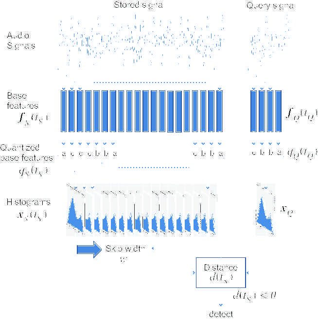
Fig. 2 outlines the Time-series Active Search (TAS) method, which is the basis of our proposed method. We provide a summary of the algorithm here. Details can be found in [11].

[Preparation stage]

1. Base features are extracted from the stored signal. Our preliminary experiments showed that the short-time frequency spectrum provides sufficient accuracy for our similarity-based search task. Base features are extracted at every sampled time step, for example, every 10 msec. Henceforth, we call the sampled points frames (the term was inspired by video frames). Base features are denoted as $\boldsymbol{f}_{S}(t_{S})$ $(0\leq t_{S}<L_{S})$, where $t_{S}$ represents the position in the stored signal and $L_{S}$ is the length of the stored signal (i.e. the number of frames in the stored signal).

2. Every base feature is quantized by vector quantization (VQ). A codebook $\{\overline{\boldsymbol{f}}_{i}\}_{i=1}^{n}$ is created beforehand, where $n$ is the codebook size (i.e. the number of codewords in the codebook). We utilize the Linde-Buzo-Gray (LBG) algorithm [16] for codebook creation. A quantized base feature $q_{S}(t_{S})$ is expressed as a VQ codeword assigned to the corresponding base feature $\boldsymbol{f}_{S}(t_{S})$, which is determined as

   $$q_{S}(t_{S}) = \arg\min_{1\leq i\leq n}\|\boldsymbol{f}_{S}(t_{S})-\overline{\boldsymbol{f}}_{i}\|^{2}.$$

[Search stage]

1. Base features $\boldsymbol{f}_{Q}(t_{Q})$ $(0\leq t_{Q}<L_{Q})$ of the query signal are extracted in the same way as the stored signal and quantized with the codebook $\{\overline{\boldsymbol{f}}_{i}\}_{i=1}^{n}$ created in the preparation stage, where $t_{Q}$ represents the position in the query signal and $L_{Q}$ is its length. We do not have to take into account the calculation time for feature quantization since it takes less than 1% of the length of the signal. A quantized base feature for the query signal is denoted as $q_{Q}(t_{Q})$.

2. Histograms are created; one for the stored signal denoted as $\boldsymbol{x}_{S}(t_{S})$ and the other for the query signal denoted as $\boldsymbol{x}_{Q}$ . First, windows are applied to the sequences of quantized base features extracted from the query and stored signals. The window length $W$ (i.e. the number of frames in the window) is set at $W=L_{Q}$, namely the length of the query signal. A histogram is created by counting the instances of each VQ codeword over the window. Therefore, each index of a histogram bin corresponds to a VQ codeword. We note that a histogram does not take the codeword order into account.

3. Histogram matching is executed based on the distance between histograms, computed as

   $$d(t_{S}) {\displaystyle\mathop{=}^{\mbox{\rm def.}}} \|\boldsymbol{x}_{S}(t_{S})-\boldsymbol{x}_{Q}\|.$$

   When the distance $d(t_{S})$ falls below a given value (search threshold) $\theta$, the query signal is considered to be detected at the position $t_{S}$ of the stored signal.

4. A window on the stored signal is shifted forward in time and the procedure returns to Step 2). As the window for the stored signal shifts forward in time, VQ codewords included in the window cannot change so rapidly, which means that histograms cannot also change so rapidly. This implies that for a given positive integer $w$ the lower bound on the distance $d(t_{S}+w)$ is obtained from the triangular inequality as follows:

   $$d(t_{S}+w) \geq \max\{0,d(t_{S})-\sqrt{2}w\},$$

   where $\sqrt{2}$ is the maximum distance between $\boldsymbol{x}_{S}(t_{S})$ and $\boldsymbol{x}_{S}(t_{S}+w)$. Therefore, the skip width $w(t_{S})$ of the window at the $t_{S}$-th frame is obtained as

   $$w(t_{S})$$ (3)

   $$= \left\{\begin{array}[]{ll}\mbox{floor}\left({\displaystyle\frac{d(t_{S})-\theta}{\sqrt{2}}}\right)+1&(\mbox{if }d(t_{S})>\theta)\\ 1,&(\mbox{otherwise})\end{array}\right.$$

   where $\mbox{floor}(a)$ indicates the largest integer less than $a$. We note that no sections will ever be missed that have distance values smaller than the search threshold $\theta$, even if we skip the width $w(t_{S})$ given by Eq. (3).

IV Framework of proposed search method

Figure 3: Overview of proposed search method.

Figure 4: Overview of the procedure for obtaining compressed features.

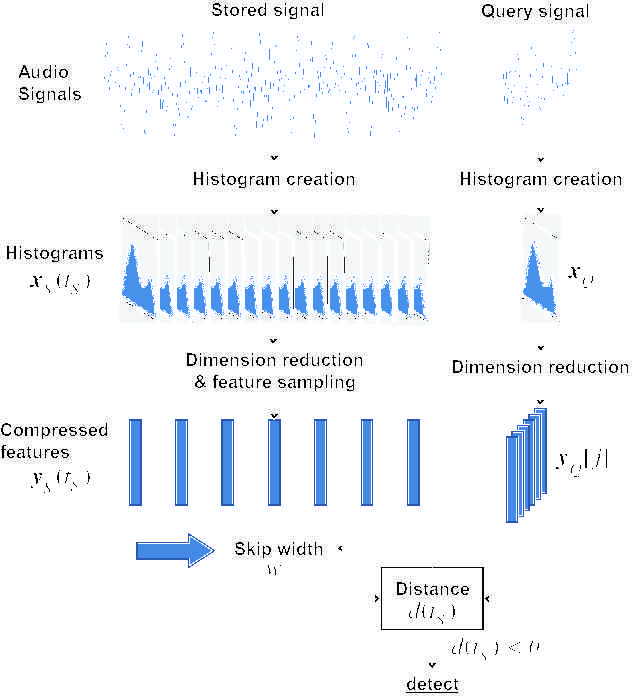
The proposed method improves the TAS method so that the search is accelerated without false dismissals (incorrectly missing segments that should be detected) or false detections (identifying incorrect matches). To accomplish this, we introduce feature-dimension reduction as explained in Sections V and VI, which reduces the calculation costs required for matching.

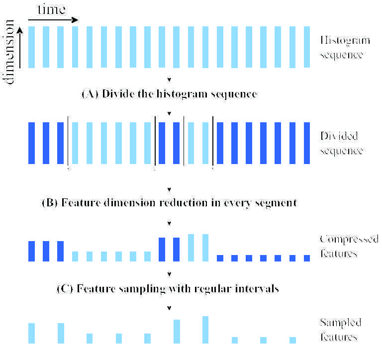
Fig. 3 shows an overview of the proposed search method, and Fig. 4 outlines the procedure for feature-dimension reduction. The procedure consists of a preparation stage and a search stage.

[Preparation stage]

1. Base features $\boldsymbol{f}_{S}(t_{S})$ are extracted from the stored signal and quantized, to create quantized base features $q_{S}(t_{S})$. The procedure is the same as that of the TAS method.

2. Histograms $\boldsymbol{x}_{S}(t_{S})$ are created in advance from the quantized base features of the stored signal by shifting a window of a predefined length $W$. We note that with the TAS method the window length $W$ varies from one search to another, while with the present method the window length $W$ is fixed. This is because histograms $\boldsymbol{x}_{S}(t_{S})$ for the stored signal are created prior to the search. We should also note that the TAS method does not create histograms prior to the search because sequences of VQ codewords need much less storage space than histogram sequences.

3. A piecewise linear representation of the extracted histogram sequence is obtained (Fig. 4 block (A)). This representation is characterized by a set $T=\{t_{j}\}_{j=0}^{M}$ of segment boundaries expressed by their frame numbers and a set $\{p_{j}(\cdot)\}_{j=1}^{M}$ of $M$ functions, where $M$ is the number of segments, $t_{0}=0$ and $t_{M}=L_{S}$. The $j$-th segment is expressed as a half-open interval $[t_{j-1},t_{j})$ since it starts from $\boldsymbol{x}_{S}(t_{j-1})$ and ends at $\boldsymbol{x}_{S}(t_{j}-1)$. Section VI shows how to obtain such segment boundaries. Each function $p_{j}(\cdot):$ $\mathcal{N}^{n}\to\mathcal{R}^{m_{j}}$ that corresponds to the $j$-th segment reduces the dimensionality $n$ of the histogram to the dimensionality $m_{j}$. Section V-B shows how to determine these functions.

4. The histograms $\boldsymbol{x}_{S}(t_{S})$ are compressed by using the functions $\{p_{j}(\cdot)\}_{j=1}^{M}$ obtained in the previous step, and then compressed features $\boldsymbol{y}_{S}(t_{S})$ are created (Fig. 4 block (B)). Section V-C details how to create compressed features.

5. The compressed features $\boldsymbol{y}_{S}(t_{S})$ are sampled at regular intervals (Fig. 4 block (C)). The details are presented in Section V-D.

[Search stage]

1. Base features $\boldsymbol{f}_{Q}(t_{Q})$ are extracted and a histogram $\boldsymbol{x}_{Q}$ is created from the query signal in the same way as the TAS method.

2. The histogram $\boldsymbol{x}_{Q}$ is compressed based on the functions $\{p_{j}(\cdot)\}_{j=1}^{M}$ obtained in the preparation stage, to create $M$ compressed features $\boldsymbol{y}_{Q}[j]$ $(j=1,\cdots,M)$. Each compressed feature $\boldsymbol{y}_{Q}[j]$ corresponds to the $j$-th function $p_{j}(\cdot)$. The procedure used to create compressed features is the same as that for the stored signal.

3. Compressed features created from the stored and query signals are matched, that is, the distance $\widetilde{d}(t_{S})=\|\boldsymbol{y}_{S}(t_{S})-\boldsymbol{y}_{Q}[j_{t_{S}}]\|$ between two compressed features $\boldsymbol{y}_{S}(t_{S})$ and $\boldsymbol{y}_{Q}[j_{t_{S}}]$ is calculated, where $j_{t_{S}}$ represents the index of the segment that contains $\boldsymbol{x}_{S}(t_{S})$, namely $t_{j_{t_{S}}-1}\leq t_{S}<t_{j_{t_{S}}}$.

4. If the distance falls below the search threshold $\theta$, the original histograms $\boldsymbol{x}_{S}(t_{S})$ corresponding to the surviving compressed features $\boldsymbol{y}_{S}(t_{S})$ are verified. Namely, the distance $d(t_{S})=\|\boldsymbol{x}_{S}(t_{S})-\boldsymbol{x}_{Q}\|$ is calculated and compared with the search threshold $\theta$.

5. A window on the stored signal is shifted forward in time and the procedure goes back to Step 3). The skip width of the window is calculated from the distance $\widetilde{d}(t_{S})$ between compressed features.

V Dimension reduction based on piecewise linear representation

V-A Related work

In most practical similarity-based searches, we cannot expect the features to be globally correlated, and therefore there is little hope of reducing dimensionality over entire feature spaces. However, even when there is no global correlation, feature subsets may exist that are locally correlated. Such local correlation of feature subsets has the potential to further reduce feature dimensionality.

A large number of dimensionality reduction methods have been proposed that focused on local correlation (e.g. [17, 18, 19, 20]). Many of these methods do not assume any specific characteristics. Now, we are concentrating on the dimensionality reduction of time-series signals, and therefore we take advantage of their continuity and local correlation. The computational cost for obtaining such feature subsets is expected to be very small compared with that of existing methods that do not utilize the continuity and local correlation of time-series signals.

Dimensionality reduction methods for time-series signals are categorized into two types: temporal dimensionality reduction, namely dimensionality reduction along the temporal axis (e.g. feature sampling), and spatial dimensionality reduction, namely the dimensionality reduction of each multi-dimensional feature sample. Keogh et al. [21, 22] and Wang et al. [23] have introduced temporal dimensionality reduction into waveform signal retrieval. Their framework considers the waveform itself as a feature for detecting similar signal segments. That is why they mainly focused on temporal dimensionality reduction. When considering audio fingerprinting, however, we handle sequences of high-dimensional features that are necessary to identify various kinds of audio segments. Thus, both spatial and temporal dimensionality reduction are required. To this end, our method mainly focuses on spatial dimensionality reduction. We also incorporate a temporal dimensionality reduction technique inspired by the method of Keogh et al. [22], which is described in Section V-D.

V-B Segment-based KL transform

Fig. 5 shows an intuitive example of a piecewise linear representation.

Figure 5: Intuitive illustration of piecewise linear representation.

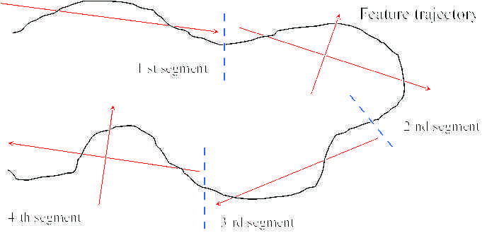
Since the histograms are created by shifting the window forward in time, successive histograms cannot change rapidly. Therefore, the histogram sequence forms a smooth trajectory in an $n$-dimensional space even if a stored audio signal includes distinct non-sequential patterns, such as irregular drum beats and intervals between music clips. This implies that a piecewise lower-dimensional representation is feasible for such a sequential histogram trajectory.

As the first step towards obtaining a piecewise representation, the histogram sequence is divided into $M$ segments. Dynamic segmentation is introduced here, which enhances feature-dimension reduction performance. This will be explained in detail in Section VI. Second, a KL transform is performed for every segment and a minimum number of eigenvectors are selected such that the sum of their contribution rates exceeds a predefined value $\sigma$, where the contribution rate of an eigenvector stands for its eigenvalue divided by the sum of all eigenvalues, and the predefined value $\sigma$ is called the contribution threshold. The number of selected eigenvectors in the $j$-th segment is written as $m_{j}$. Then, a function $p_{j}(\cdot):$ $\mathcal{N}^{n}\to\mathcal{R}^{m_{j}}$ $(j=1,2,\cdots,M)$ for dimensionality reduction is determined as a map to a subspace whose bases are the selected eigenvectors:

$$p_{j}(\boldsymbol{x}) = \boldsymbol{P}_{j}^{t}(\boldsymbol{x}-\overline{\boldsymbol{x}}_{j}),$$ (4)

where $\boldsymbol{x}$ is a histogram, $\overline{\boldsymbol{x}}_{j}$ is the centroid of histograms contained in the $j$-th segment, and $\boldsymbol{P}_{j}$ is an ($n\times m_{j}$) matrix whose columns are the selected eigenvectors. Finally, each histogram is compressed by using the function $p_{j}(\cdot)$ of the segment to which the histogram belongs. Henceforth, we refer to $p_{j}(\boldsymbol{x})$ as a projected feature of a histogram $\boldsymbol{x}$.

In the following, we omit the index $j$ corresponding to a segment unless it is specifically needed, e.g. $p(\boldsymbol{x})$ and $\overline{\boldsymbol{x}}$.

V-C Distance bounding

From the nature of the KL transform, the distance between two projected features gives the lower bound of the distance between corresponding original histograms. However, this bound does not approximate the original distance well, and this results in many false detections.

To improve the distance bound, we introduce a new technique. Let us define a projection distance $\delta(p,\boldsymbol{x})$ as the distance between a histogram $\boldsymbol{x}$ and the corresponding projected feature $\boldsymbol{z}=p(\boldsymbol{x})$:

$$\delta(p,\boldsymbol{x}) {\displaystyle\mathop{=}^{\mbox{\rm def.}}} \|\boldsymbol{x}-q(\boldsymbol{z})\|,$$ (5)

where $q(\cdot):\mathcal{R}^{m}\to\mathcal{R}^{n}$ is the generalized inverse map of $p(\cdot)$, defined as

$$q(\boldsymbol{z}) {\displaystyle\mathop{=}^{\mbox{\rm def.}}} \boldsymbol{P}\boldsymbol{z}+\overline{\boldsymbol{x}}.$$

Here we create a compressed feature $\boldsymbol{y}$, which is the projected feature $\boldsymbol{z}=(z_{1},z_{2},\cdots,z_{m})^{t}$ along with the projection distance $\delta(p,\boldsymbol{x})$:

$$\boldsymbol{y}=\boldsymbol{y}(p,\boldsymbol{x}) = (z_{1},z_{2},\cdots,z_{m},\delta(p,\boldsymbol{x}))^{t},$$

where $\boldsymbol{y}(p,\boldsymbol{x})$ means that $\boldsymbol{y}$ is determined by $p$ and $\boldsymbol{x}$. The Euclidean distance between compressed features is utilized as a new criterion for matching instead of the Euclidean distance between projected features. The distance is expressed as

$$\|\boldsymbol{y}_{S}-\boldsymbol{y}_{Q}\|^{2}$$ (6)

$$= \|\boldsymbol{z}_{S}-\boldsymbol{z}_{Q}\|^{2}+\{\delta(p,\boldsymbol{x}_{S})-\delta(p,\boldsymbol{x}_{Q})\}^{2},$$

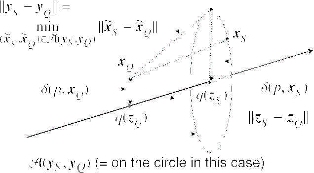
where $\boldsymbol{z}_{S}=p(\boldsymbol{x}_{S})$ (resp. $\boldsymbol{z}_{Q}=p(\boldsymbol{x}_{Q})$) is the project feature derived from the original histograms $\boldsymbol{x}_{S}$ (resp. $\boldsymbol{x}_{Q}$) and $\boldsymbol{y}_{S}=\boldsymbol{y}_{S}(p,\boldsymbol{x}_{S})$ (resp. $\boldsymbol{y}_{Q}=\boldsymbol{y}_{Q}(p,\boldsymbol{x}_{Q})$) is the corresponding compressed feature. Eq. (6) implies that the distance between compressed features is larger than the distance between corresponding projected features. In addition, from the above discussions, we have the following two properties, which indicate that the distance $\|\boldsymbol{y}_{S}-\boldsymbol{y}_{Q}\|$ between two compressed features is a better approximation of the distance $\|\boldsymbol{x}_{S}-\boldsymbol{x}_{Q}\|$ between the original histograms than the distance $\|\boldsymbol{z}_{S}-\boldsymbol{z}_{Q}\|$ between projected features (Theorem 1), and the expected approximation error is much smaller (Theorem 2).

Figure 6: Intuitive illustration of relationships between projection distance, distance between projected features and distance between compressed features.

Theorem 1

$$\|\boldsymbol{z}_{S}-\boldsymbol{z}_{Q}\|\leq\|\boldsymbol{y}_{S}-\boldsymbol{y}_{Q}\|$$ (7)

$$= \min_{(\tilde{\boldsymbol{x}}_{S},\tilde{\boldsymbol{x}}_{Q})\in\mathcal{A}(\boldsymbol{y}_{S},\boldsymbol{y}_{Q})}\|\tilde{\boldsymbol{x}}_{S}-\tilde{\boldsymbol{x}}_{Q}\|\leq\|\boldsymbol{x}_{S}-\boldsymbol{x}_{Q}\|,$$

where $\mathcal{A}(\boldsymbol{y}_{S},\boldsymbol{y}_{Q})$ is the set of all possible pairs $(\tilde{\boldsymbol{x}}_{S},\tilde{\boldsymbol{x}}_{Q})$ of original histograms for given compressed features $(\boldsymbol{y}_{S},\boldsymbol{y}_{Q})$.

Theorem 2

Suppose that random variables $(X_{S}^{n},X_{Q}^{n})$ corresponding to the original histograms $(\boldsymbol{x}_{S},\boldsymbol{x}_{Q})$ have a uniform distribution on the set $\mathcal{A}(\boldsymbol{y}_{S},\boldsymbol{y}_{Q})$ defined in Theorem 1, and $E[\delta(p,X_{S}^{n})]\gg E[\delta(p,X_{Q}^{n})]$. The expected approximation errors can be evaluated as

$$E\left[\left.\|X_{S}^{n}-X_{Q}^{n}\|^{2}-\|\boldsymbol{y}_{S}-\boldsymbol{y}_{Q}\|^{2}\right|\boldsymbol{y}_{S},\boldsymbol{y}_{Q}\right]$$ (8)

$$\ll E\left[\left.\|X_{S}^{n}-X_{Q}^{n}\|^{2}-\|\boldsymbol{z}_{S}-\boldsymbol{z}_{Q}\|^{2}\right|\boldsymbol{y}_{S},\boldsymbol{y}_{Q}\right].$$

The proofs are shown in the appendix. Fig. 6 shows an intuitive illustration of the relationships between projection distances, distances between projected features and distances between compressed features, where the histograms are in a 3-dimensional space and the subspace dimensionality is 1. In this case, for given compressed features $(\boldsymbol{y}_{S},\boldsymbol{y}_{Q})$ and a fixed query histogram $\boldsymbol{x}_{Q}$, a stored histogram $\boldsymbol{x}_{S}$ must be on a circle whose center is $q(\boldsymbol{z}_{Q})$. This circle corresponds to the set $\mathcal{A}(\boldsymbol{y}_{S},\boldsymbol{y}_{Q})$.

V-D Feature sampling

In the TAS method, quantized base features are stored, because they need much less storage space than the histogram sequence and creating histograms on the spot takes little calculation. With the present method, however, compressed features must be computed and stored in advance so that the search results can be returned as quickly as possible, and therefore much more storage space is needed than with the TAS method. The increase in storage space may cause a reduction in search speed due to the increase in disk access.

Based on the above discussion, we incorporate feature sampling in the temporal domain. The following idea is inspired by the technique called Piecewise Aggregate Approximation (PAA) [22]. With the proposed feature sampling method, first a compressed feature sequence $\{\boldsymbol{y}_{S}(t_{S})\}_{t_{S}=0}^{L_{S}-W-1}$ is divided into subsequences

$$\{\boldsymbol{y}_{S}(ia),\boldsymbol{y}_{S}(ia+1),\cdots,\boldsymbol{y}_{S}(ia+a-1)\}_{i=0,1,\cdots}$$

of length $a$. Then, the first compressed feature $\boldsymbol{y}_{S}(ia)$ of every subsequence is selected as a representative feature. A lower bound of the distances between the query and stored compressed features contained in the subsequence can be expressed in terms of the representative feature $\boldsymbol{y}_{S}(ia)$. This bound is obtained from the triangular inequality as follows:

$$\|\boldsymbol{y}_{S}(ia+k)-\boldsymbol{y}_{Q}\|\geq\|\boldsymbol{y}_{S}(ia)-\boldsymbol{y}_{Q}\|-\overline{d}(i),$$

$$\overline{d}(i){\displaystyle\mathop{=}^{\mbox{\rm def.}}}\max_{0\leq k^{\prime}\leq a-1}\|\boldsymbol{y}_{S}(ia+k^{\prime})-\boldsymbol{y}_{S}(ia)\|.$$

$$\hskip 42.67912pt(\forall i=0,1,\cdots,\quad\forall k=0,\cdots,a-1)$$

This implies that preserving the representative feature $\boldsymbol{y}_{S}(ia)$ and the maximum distance $\overline{d}(i)$ is sufficient to guarantee that there are no false dismissals.

This feature sampling is feasible for histogram sequences because successive histograms cannot change rapidly. Furthermore, the technique mentioned in this section will also contribute to accelerating the search, especially when successive histograms change little.

VI Dynamic segmentation

VI-A Related work

The approach used for dividing histogram sequences into segments is critical for realizing efficient feature-dimension reduction since the KL transform is most effective when the constituent elements in the histogram segments are similar. To achieve this, we introduce a dynamic segmentation strategy.

Dynamic segmentation is a generic term that refers to techniques for dividing sequences into segments of various lengths. Dynamic segmentation methods for time-series signals have already been applied to various kinds of applications such as speech coding (e.g. [24]), the temporal compression of waveform signals [25], the automatic segmentation of speech signals into phonic units [26], sinusoidal modeling of audio signals [27, 28, 29] and motion segmentation in video signals [30]. We employ dynamic segmentation to minimize the average dimensionality of high-dimensional feature trajectories.

Dynamic segmentation can improve dimension reduction performance. However, finding the optimal boundaries still requires a substantial calculation. With this in mind, several studies have adopted suboptimal approaches, such as longest line fitting [23], wavelet decomposition [23, 21] and the bottom-up merging of segments [31]. The first two approaches still incur a substantial calculation cost for long time-series signals. The last approach is promising as regards obtaining a rough global approximation at a practical calculation cost. This method is compatible with ours, however, we mainly focus on a more precise local optimization.

VI-B Framework

Figure 7: Outline of dynamic segmentation.

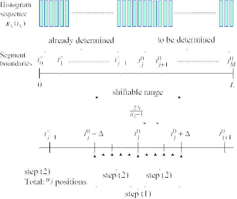
Fig. 7 shows an outline of our dynamic segmentation method. The objective of the dynamic segmentation method is to divide the stored histogram sequence so that its piecewise linear representation is well characterized by a set of lower dimensional subspaces. To this end, we formulate the dynamic segmentation as a way to find a set $T^{*}=\{t_{j}^{*}\}_{j=0}^{M}$ of segment boundaries that minimize the average dimensionality of these segment-approximating subspaces on condition that the boundary $t_{j}^{*}$ between the $j$-th and the $(j+1)$-th segments is in a shiftable range $S_{j}$, which is defined as a section with a width $\Delta$ in the vicinity of the initial position $t_{j}^{0}$ of the boundary between the $j$-th and the $(j+1)$-th segments. Namely, the set $T^{*}$ of the optimal segment boundaries is given by the following formula:

$$T^{*} = \left\{t_{j}^{*}\right\}_{j=0}^{M}$$ (9)

$${\displaystyle\mathop{=}^{\mbox{\rm def.}}} {\displaystyle\mathop{\arg\min}_{\{t_{j}\}_{j=0}^{M}:t_{j}\in S_{j}\forall j}}\frac{1}{L_{S}}\sum_{i=1}^{M}(t_{j}-t_{j-1})\cdot c(t_{j-1},t_{j},\sigma)$$

$$S_{j} {\displaystyle\mathop{=}^{\rm def.}} \{t_{j}:t_{j}^{0}-\Delta\leq t_{j}\leq t_{j}^{0}+\Delta\}$$ (10)

where $c(t_{i},t_{j},\sigma)$ represents the subspace dimensionality on the segment between the $t_{i}$-th and the $t_{j}$-th frames for a given contribution threshold $\sigma$, $t_{0}^{*}=0$ and $t_{M}^{*}=L_{S}$. The initial positions of the segment boundaries are set beforehand by equi-partitioning.

The above optimization problem defined by Eq. (9) would normally be solved with dynamic programming (DP) (e.g. [32]). However, DP is not practical in this case. Deriving $c(t_{j-1},t_{j},\sigma)$ included in Eq. (9) incurs a substantial calculation cost since it is equivalent to executing a KL transform calculation for the segment $[t_{j-1},t_{j})$. This implies that the DP-based approach requires a significant amount of calculation, although less than a naive approach. The above discussion implies that we should reduce the number of KL transform calculations to reduce the total calculation cost required for the optimization. When we adopt the total number of KL transform calculations as a measure for assessing the calculation cost, the cost is evaluated as $\mathcal{O}(M\Delta^{2})$, where $M$ is the number of segments and $\Delta$ is the width of the shiftable range.

To reduce the calculation cost, we instead adopt a suboptimal approach. Two techniques are incorporated: local optimization and the coarse-to-fine detection of segment boundaries. We explain these two techniques in the following sections.

VI-C Local optimization

The local optimization technique modifies the formulation (Eq. (9)) of dynamic segmentation so that it minimizes the average dimensionality of the subspaces of adjoining segments. The basic idea is similar to the “forward segmentation” technique introduced by Goodwin [27, 28] for deriving accurate sinusoidal models of audio signals. The position $t_{j}^{*}$ of the boundary is determined by using the following forward recursion as a substitute for Eq. (9):

$$t_{j}^{*} = \arg\min_{t_{j}\in S_{j}}\frac{(t_{j}-t_{j-1}^{*})c_{j}^{*}+(t_{j+1}^{0}-t_{j})c_{j+1}^{0}}{t_{j+1}^{0}-t_{j-1}^{*}},$$ (11)

which is here given by

$$c_{j}^{*}=c(t_{j-1}^{*},t_{j},\sigma),\ c_{j+1}^{0}=c(t_{j},t_{j+1}^{0},\sigma),$$

and $S_{j}$ is defined in Eq. (10). As can be seen in Eq. (11), we can determine each segment boundary independently, unlike the formulation of Eq. (9). Therefore, the local optimization technique can reduce the amount of calculation needed for extracting an appropriate representation, which is evaluated as $\mathcal{O}(M\Delta)$, where $M$ is the number of segments and $\Delta$ is the width of the shiftable range.

VI-D Coarse-to-fine detection

The coarse-to-fine detection technique selects suboptimal boundaries in the sense of Eq. (11) with less computational cost. We note that small boundary shifts do not contribute greatly to changes in segment dimensionality because successive histograms cannot change rapidly. With this in mind, we assume that the optimal positions of the segment boundaries are at the edges of the shiftable range or at the points where dimensions change. Figs. 9 and 9 show two intuitive examples where the optimal position of the segment boundary may be at the point where dimensionality changes.

Figure 8: Example 1: $c(t_{j},t_{j+1}^{0},\sigma)$ decreases when the boundary $t_{j}$ is shifted forward in time.

Figure 9: Example 2: $c(t_{j-1}^{*},t_{j},\sigma)$ increases when the boundary $t_{j}$ is shifted forward in time.

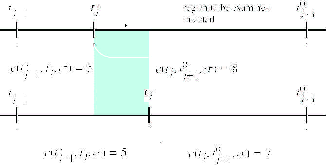
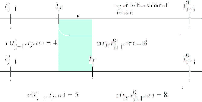
The coarse-to-fine detection technique quickly finds the points where the dimensions change. The procedure for this technique has three steps.

1. The dimensions of the $j$-th and $(j+1)$-th segments are calculated when the segment boundary $t_{j}$ is at the initial position $t_{j}^{0}$ and the edges ($t_{j}^{0}-\Delta$ and $t_{j}^{0}+\Delta$) of its shiftable range.

2. The dimensions of the $j$-th and $(j+1)$-th segments are calculated when the segment boundary $t_{j}$ is at the position $t_{j}^{0}-\Delta+\frac{2\Delta}{u_{j}+1}i$ $(i=1,2,\cdots,u_{j})$, where $u_{j}$ determines the number of calculations in this step.

3. The dimensions of the $j$-th and $(j+1)$-th segments are calculated in detail when the segment boundary $t_{j}$ is in the positions where dimension changes are detected in the previous step.

We determine the number $u_{j}$ of dimension calculations in step 2 so that the number of calculations in all the above steps, $f_{j}(u_{j})$, is minimized. Then, $f_{j}(u_{j})$ is given as follows:

$$f_{j}(u_{j})=2\left((3+u_{j})+K_{j}\frac{\Delta}{\frac{1}{2}u_{j}+1}\right),$$

where $K_{j}$ is the estimated number of positions where the dimensionalities change, which is experimentally determined as

$$K_{j} = c_{LR}-c_{LL},$$

$$(\mbox{if }c_{LR}\leq c_{RR},c_{LL}<c_{RL})$$

$$K_{j} = (c_{LC}-c_{LL})+\min(c_{RC},c_{LR})-\min(c_{LC},c_{RR}),$$

$$(\mbox{if }c_{LR}>c_{RR},c_{LL}<c_{RL},c_{LC}\leq c_{RC})$$

$$K_{j} = (c_{RC}-c_{RR})+\min(c_{LC},c_{RL})-\min(c_{RC},c_{LL}),$$

$$(\mbox{if }c_{LR}>c_{RR},c_{LL}<c_{RL},c_{LC}>c_{RC})$$

$$K_{j} = c_{RL}-c_{RR},\quad(\mbox{Otherwise})$$

and

$$\begin{array}[]{ll}c_{LL}=c(t_{j-1}^{*},t_{j}^{0}-\Delta,\sigma),&c_{RL}=c(t_{j}^{0}-\Delta,t_{j+1}^{0},\sigma),\\ c_{LC}=c(t_{j-1}^{*},t_{j}^{0},\sigma),&c_{RC}=c(t_{j}^{0},t_{j+1}^{0},\sigma),\\ c_{LR}=c(t_{j-1}^{*},t_{j}^{0}+\Delta,\sigma),&c_{RR}=c(t_{j}^{0}+\Delta,t_{j+1}^{0},\sigma).\end{array}$$

The first term of $f_{j}(u_{j})$ refers to the number of calculations in steps 1 and 2, and the second term corresponds to that in step 3. $f_{j}(u_{j})$ takes the minimum value $4\sqrt{2K_{j}\Delta}+2$ when $u_{j}=\sqrt{2K_{j}\Delta}-2$. The calculation cost when incorporating local optimization and coarse-to-fine detection techniques is evaluated as follows:

$$E\left[M\left(4\sqrt{2K_{j}\Delta}+2\right)\right] \leq M\left(4\sqrt{2K\Delta}+2\right)$$

$$= {\cal O}\left(M\sqrt{K\Delta}\right),$$

where $K=E[K_{j}]$, $M$ is the number of segments and $\Delta$ is the width of the shiftable range. The first inequality is derived from Jensen’s inequality (e.g. [33, Theorem 2.6.2]). The coarse-to-fine detection technique can additionally reduce the calculation cost because $K$ is usually much smaller than $\Delta$.

VII Experiments

VII-A Conditions

We tested the proposed method in terms of calculation cost in relation to search speed. We again note that the proposed search method guarantees the same search results as the TAS method in principle, and therefore we need to evaluate the search speed. The search accuracy for the TAS method was reported in a previous paper [11]. In summary, for audio identification tasks, there were no false detections or false dismissals down to an S/N ratio of 20 dB if the query duration was longer than 10 seconds.

In the experiments, we used a recording of a real TV broadcast. An audio signal broadcast from a particular TV station was recorded and encoded in MPEG-1 Layer 3 (MP3) format. We recorded a 200-hour audio signal as a stored signal, and recorded 200 15-second spots from another TV broadcast as queries. Thus, the task was to detect and locate specific commercial spots from 200 consecutive hours of TV recording. Each spot occurred 2-30 times in the stored signal. Each signal was first digitized at a 32 kHz sampling frequency and 16 bit quantization accuracy. The bit rate for the MP3 encoding was 56 kbps. We extracted base features from each audio signal using a 7-channel second-order IIR band-pass filter with $Q=10$. The center frequencies at the filter were equally spaced on a log frequency scale. The base features were calculated every 10 milliseconds from a 60 millisecond window. The base feature vectors were quantized by using the VQ codebook with 128 codewords, and histograms were created based on the scheme of the TAS method. Therefore, the histogram dimension was 128. We implemented the feature sampling described in Section V-D and the sampling duration was $a=50$. The tests were carried out on a PC (Pentium 4 2.0 GHz).

VII-B Search speed

We first measured the CPU time and the number of matches in the search. The search time we measured in this test comprised only the CPU time in the search stage shown in Section IV. This means that the search time did not include the CPU time for any procedures in the preparation stage such as base feature extraction, histogram creation, or histogram dimension reduction for the stored signal. The search threshold was adjusted to $\theta=85$ so that there were no false detections or false dismissals. We compared the following methods:

1. The TAS method (baseline).

2. The proposed search method without the projection distance being embedded in the compressed features.

3. The proposed search method.

Figure 10: Relationship between average segment duration and search speed measured by the CPU time in the search: (Horizontal axis) Average segment duration [200 hours - 1.2 minutes], which corresponds to the number of segments [1 - 10000], (Vertical axis) the CPU time in the search and the speed-up factor.

Figure 11: Relationship between average segment duration and search speed measured by number of matches: (Horizontal axis) Average segment duration [200 hours - 1.2 minutes], which corresponds to the number of segments [1 - 10000], (Vertical axis) Number of matches.

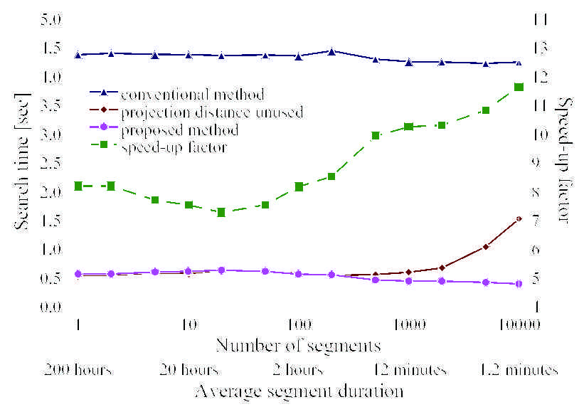
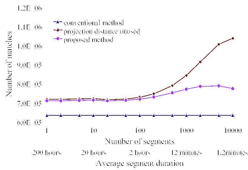
We first examined the relationships between the average segment duration (equivalent to the number of segments), the search time, and the number of matches. The following parameters were set for feature-dimension reduction: The contribution threshold was $\sigma=0.9$. The width of the shiftable range for dynamic segmentation was 500.

Fig. 10 shows the relationship between the average segment duration and the search time, where the ratio of the search speed of the proposed method to that of the TAS method (conventional method in the figure) is called the speed-up factor. Also, Fig. 11 shows the relationship between the average segment duration and the number of matches. Although the proposed method only slightly increased the number of matches, it greatly reduced the search time. This is because it greatly reduced the calculation cost per match owing to feature-dimension reduction. For example, the proposed method reduced the search time to almost $1/12$ when the segment duration was 1.2 minutes (i.e. the number of segments was $10000$). As mentioned in Section V-D, the feature sampling technique also contributed to the acceleration of the search, and the effect is similar to histogram skipping. Considering the dimension reduction performance results described later, we found that those effects were greater than that caused by dimension reduction for large segment durations (i.e. a small number of segments). This is examined in detail in the next section. We also found that the proposed method reduced the search time and the number of matches when the distance bounding technique was incorporated, especially when there were a large number of segments.

VIII Discussion

The previous section described the experimental results solely in terms of search speed and the advantages of the proposed method compared with the previous method. This section provides further discussion of the advantages and shortcomings of the proposed method as well as additional experimental results.

Figure 12: Dimension reduction performance based on contribution rates: (Horizontal axis) Segment duration [200 hours - 1.2 minutes], which corresponds to the number of segments [1 - 10000] (Vertical axis) Average dimensionality of projected features per sample.

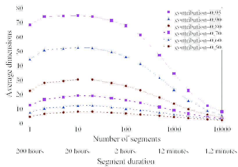
We first deal with the dimension reduction performance derived from the segment-based KL transform. We employed equi-partitioning to obtain segments, which means that we did not incorporate the dynamic segmentation technique. Fig. 12 shows the experimental result. The proposed method monotonically reduced the dimensions as the number of segments increased if the segment duration was shorter than 10 hours (the number of segments $M\geq 20$). We can see that the proposed method reduced the dimensions, for example, to $1/25$ of the original histograms when the contribution threshold was $0.90$ and the segment duration was 1.2 minutes (the number of segments was $10000$). The average dimensions did not decrease as the number of segments increased if the number of segments was relatively small. This is because we decided the number of subspace bases based on the contribution rates.

Figure 13: Dimension reduction performance of dynamic segmentation [Number of segments$=1000$, contribution rate$=0.9$]: (Horizontal axis) Width of shiftable range [1 - 5000] (Vertical axis) Proportion of the dimensionality derived from dynamic segmentation compared with that obtained in the initial state (i.e. equi-partitioning).

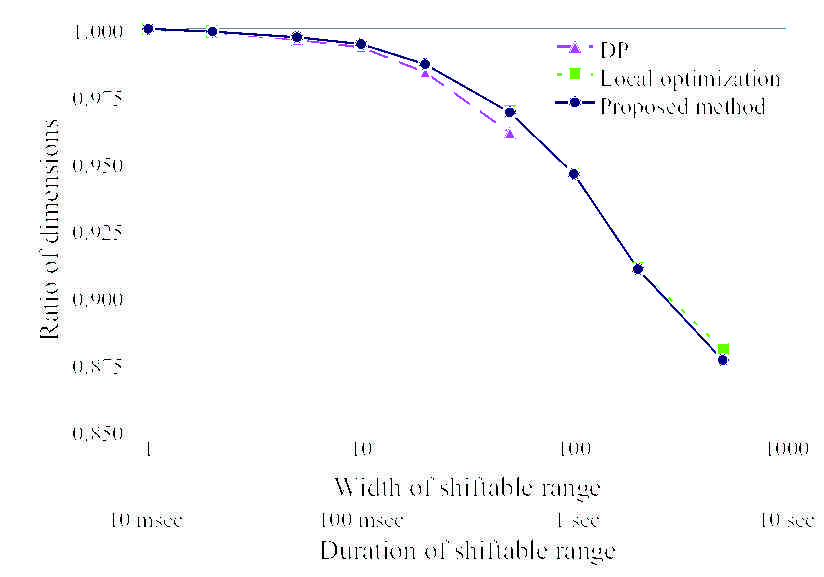
Next, we deal with the dimension reduction performance derived from the dynamic segmentation technique. The initial positions of the segment boundaries were set by equi-partitioning. The duration of segments obtained by equi-partitioning was 12 minutes (i.e. there were $1000$ segments). Fig. 13 shows the result. The proposed method further reduced the feature dimensionality to $87.5\%$ of its initial value, which is almost the same level of performance as when only the local search was utilized. We were unable to calculate the average dimensionality when using DP because of the substantial amount of calculation, as described later. When the shiftable range was relatively narrow, the dynamic segmentation performance was almost the same as that of DP.

Here, we review the search speed performance shown in Fig. 10. It should be noted that three techniques in our proposed method contributed to speeding up the search, namely feature-dimension reduction, distance bounding and feature sampling. When the number of segments was relatively small, the speed-up factor was much larger than the ratio of the dimension of the compressed features to that of the original histograms, which can be seen in Figs. 10, 12 and 13. This implies that the feature sampling technique dominated the search performance in this case. On the other hand, when the number of segments was relatively large, the proposed search method did not greatly improve the search speed compared with the dimension reduction performance. This implies that the feature sampling technique degraded the search performance. In this case, the distance bounding technique mainly contributed to the improvement of the search performance as seen in Fig. 10.

Figure 14: Amount of computation for dynamic segmentation [Number of segments$=1000$, contribution rate$=0.9$] (Horizontal axis) Width of shiftable range [1 - 1000] (Vertical axis) Total number of PCA calculations needed to obtain the representation, where the horizontal line along with “Real-time processing” indicates that the computational time is almost the same as the duration of the stored signal.

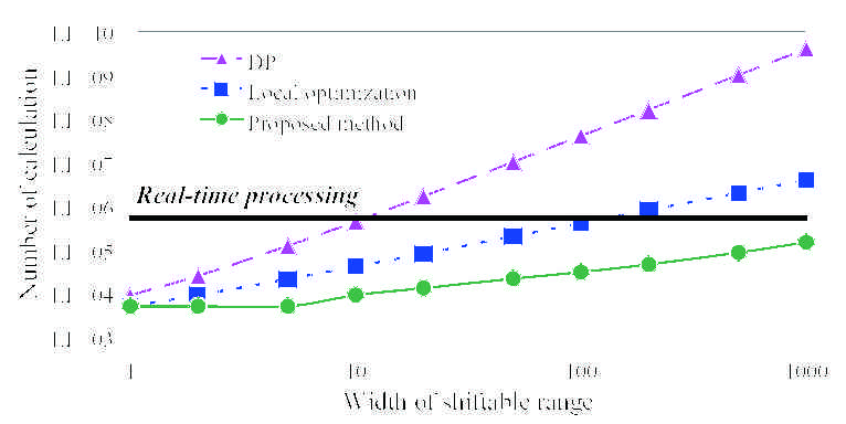
Lastly, we discuss the amount of calculation necessary for dynamic segmentation. We again note that although dynamic segmentation can be executed prior to providing a query signal, the computational time must be at worst smaller than the duration of the stored signal from the viewpoint of practical applicability. We adopted the total number of dimension calculations needed to obtain the dimensions of the segments as a measure for comparing the calculation cost in the same way as in Section VI. Fig. 14 shows the estimated calculation cost for each dynamic segmentation method. We compared our method incorporating local optimization and coarse-to-fine detection with the DP-based method and a case where only the local optimization technique was incorporated. The horizontal line along with “Real-time processing” indicates that the computational time is almost the same as the duration of the signal. The proposed method required much less computation than with DP or local optimization. For example, when the width of the shiftable range was 500, the calculation cost of the proposed method was $1/5000$ that of DP and $1/10$ that with local optimization. We note that in this experiment, the calculation cost of the proposed method is less than the duration of the stored signal, while those of the other two methods are much longer.

IX Concluding remarks

This paper proposed a method for undertaking quick similarity-based searches of an audio signal to detect and locate similar segments to a given audio clip. The proposed method was built on the TAS method, where audio segments are modeled by using histograms. With the proposed method, the histograms are compressed based on a piecewise linear representation of histogram sequences. We introduce dynamic segmentation, which divides histogram sequences into segments of variable lengths. We also addressed the quick suboptimal partitioning of the histogram sequences along with local optimization and coarse-to-fine detection techniques. Experiments revealed significant improvements in search speed. For example, the proposed method reduced the total search time to approximately $1/12$, and detected the query in about $0.3$ seconds from a 200-hour audio database. Although this paper focused on audio signal retrieval, the proposed method can be easily applied to video signal retrieval [34, 35]. Although the method proposed in this paper is founded on the TAS method, we expect that some of the techniques we have described could be used in conjunction with other similarity-based search methods (e.g. [36, 37, 38, 39]) or a speech/music discriminator [40]. Future work includes the implementation of indexing methods suitable for piecewise linear representation, and the dynamic determination of the initial segmentation, both of which have the potential to improve the search performance further.

Appendix A Proof of Theorem 1

First, let us define

$$\boldsymbol{z}_{Q}{\displaystyle\mathop{=}^{\mbox{\rm def.}}}p(\boldsymbol{x}_{Q}),\quad\boldsymbol{z}_{S}{\displaystyle\mathop{=}^{\mbox{\rm def.}}}p(\boldsymbol{x}_{S}),$$

$$\widehat{\boldsymbol{x}}_{Q}{\displaystyle\mathop{=}^{\mbox{\rm def.}}}q(\boldsymbol{z}_{Q})=q(p(\boldsymbol{x}_{Q})),\quad\widehat{\boldsymbol{x}}_{S}{\displaystyle\mathop{=}^{\mbox{\rm def.}}}q(\boldsymbol{z}_{S})=q(p(\boldsymbol{x}_{S})),$$

$$\delta_{Q}{\displaystyle\mathop{=}^{\mbox{\rm def.}}}\delta(p,\boldsymbol{x}_{Q}),\quad\delta_{S}{\displaystyle\mathop{=}^{\mbox{\rm def.}}}\delta(p,\boldsymbol{x}_{S}).$$

We note that for any histogram $\boldsymbol{x}\in\mathcal{N}^{n}$, $\widehat{\boldsymbol{x}}=q(p(\boldsymbol{x}))$ is the projection of $\boldsymbol{x}$ into the subspace defined by the map $p(\cdot)$, and therefore $\boldsymbol{x}-\widehat{\boldsymbol{x}}$ is a normal vector of the subspace of $p(\cdot)$. Also, we note that $\|\boldsymbol{x}-\widehat{\boldsymbol{x}}\|=\delta(p,\boldsymbol{x})$ and $\widehat{\boldsymbol{x}}$ is on the subspace of $p(\cdot)$. For two vectors $\boldsymbol{x}_{1}$ and $\boldsymbol{x}_{2}$, their inner product is denoted as $\boldsymbol{x}_{1}\cdot\boldsymbol{x}_{2}$. Then, we obtain

$$\|\boldsymbol{x}_{Q}-\boldsymbol{x}_{S}\|^{2}$$

$$= \|(\boldsymbol{x}_{Q}-\widehat{\boldsymbol{x}}_{Q})-(\boldsymbol{x}_{S}-\widehat{\boldsymbol{x}}_{S})+(\widehat{\boldsymbol{x}}_{Q}-\widehat{\boldsymbol{x}}_{S})\|^{2}$$

$$= \|\boldsymbol{x}_{Q}-\widehat{\boldsymbol{x}}_{Q}\|^{2}+\|\boldsymbol{x}_{S}-\widehat{\boldsymbol{x}}_{S}\|^{2}+\|\widehat{\boldsymbol{x}}_{Q}-\widehat{\boldsymbol{x}}_{S}\|^{2}$$

$$-2(\boldsymbol{x}_{Q}-\widehat{\boldsymbol{x}}_{Q})\cdot(\boldsymbol{x}_{S}-\widehat{\boldsymbol{x}}_{S})+2(\boldsymbol{x}_{Q}-\widehat{\boldsymbol{x}}_{Q})\cdot(\widehat{\boldsymbol{x}}_{Q}-\widehat{\boldsymbol{x}}_{S})$$

$$-2(\boldsymbol{x}_{S}-\widehat{\boldsymbol{x}}_{S})\cdot(\widehat{\boldsymbol{x}}_{Q}-\widehat{\boldsymbol{x}}_{S})$$

$$= \delta(p,\boldsymbol{x}_{Q})^{2}+\delta(p,\boldsymbol{x}_{S})^{2}+\|\widehat{\boldsymbol{x}}_{Q}-\widehat{\boldsymbol{x}}_{S}\|^{2}$$

$$-2(\boldsymbol{x}_{Q}-\widehat{\boldsymbol{x}}_{Q})\cdot(\boldsymbol{x}_{S}-\widehat{x}_{S})$$

$$\geq \delta(p,\boldsymbol{x}_{Q})^{2}+\delta(p,\boldsymbol{x}_{S})^{2}+\|\widehat{\boldsymbol{x}}_{Q}-\widehat{\boldsymbol{x}}_{S}\|^{2}$$

$$-2\delta(p,\boldsymbol{x}_{Q})\cdot\delta(p,\boldsymbol{x}_{S})$$

$$= \{\delta(p,\boldsymbol{x}_{Q})-\delta(p,\boldsymbol{x}_{S})\}^{2}+\|\boldsymbol{z}_{Q}-\boldsymbol{z}_{S}\|^{2}$$

$$= \|\boldsymbol{y}_{Q}-\boldsymbol{y}_{S}\|^{2},$$

where Eq. (A) comes from the fact that any vector on a subspace and the normal vector of the subspace are mutually orthogonal, and Eq. (A) from the definition of inner product. This concludes the proof of Theorem 1.

Appendix B Proof of Theorem 2

The notations used in the previous section are also employed here. When the projected features $\boldsymbol{z}_{Q}$, $\boldsymbol{z}_{S}$ and the projection distances

$$\delta_{Q}{\displaystyle\mathop{=}^{\mbox{\rm def.}}}\delta(p,\boldsymbol{x}_{Q}),\quad\delta_{S}{\displaystyle\mathop{=}^{\mbox{\rm def.}}}\delta(p,\boldsymbol{x}_{S})$$

are given, we can obtain the distance between the original features as follows:

$$\|\boldsymbol{x}_{Q}-\boldsymbol{x}_{S}\|^{2}$$

$$= \|\boldsymbol{z}_{Q}-\boldsymbol{z}_{S}\|^{2}+\delta_{Q}^{2}+\delta_{S}^{2}$$

$$-(\boldsymbol{x}_{Q}-q(\boldsymbol{z}_{Q}))\cdot(\boldsymbol{x}_{S}-q(\boldsymbol{z}_{S}))$$

$$= \|\boldsymbol{z}_{Q}-\boldsymbol{z}_{S}\|^{2}+\delta_{Q}^{2}+\delta_{S}^{2}-2\delta_{Q}\delta_{S}\cos\phi,$$

where Eq. (B) is derived from Eq. (A) and $\phi$ is the angle between $\boldsymbol{x}_{Q}-q(\boldsymbol{z}_{Q})$ and $\boldsymbol{x}_{S}-q(\boldsymbol{z}_{S})$. From the assumption that random variables $\boldsymbol{X}_{S}$ and $\boldsymbol{X}_{Q}$ corresponding to original histograms $\boldsymbol{x}_{S}$ and $\boldsymbol{x}_{Q}$ are distributed independently and uniformly in the set $\mathcal{A}$, the following equation is obtained:

$$E\left[\|\boldsymbol{X}_{Q}-\boldsymbol{X}_{S}\|^{2}-\|\boldsymbol{z}_{Q}-\boldsymbol{z}_{S}\|^{2}\right]$$ (16)

$$= \int_{0}^{\pi}(\delta_{Q}^{2}+\delta_{S}^{2}-2\delta_{Q}\delta_{S}\cos\phi)$$

$$\hskip 17.07164pt\frac{S_{n-m-1}(\delta_{S}\sin\phi)}{S_{n-m}(\delta_{S})}|d(\delta_{S}\cos\phi)|,$$

where $S_{k}(R)$ represents the surface area of a $k$-dimensional hypersphere with radius $R$, and can be calculated as follows:

$$S_{k}(R) = k\frac{\pi^{k/2}}{(k/2)!}R^{k-1}$$ (17)

Substituting Eq. (17) into Eq. (16), we obtain

$$E\left[\|\boldsymbol{X}_{Q}-\boldsymbol{X}_{S}\|^{2}-\|\boldsymbol{z}_{Q}-\boldsymbol{z}_{S}\|^{2}\right]$$

$$= \frac{n-m-1}{n-m}(\delta_{Q}^{2}+\delta_{S}^{2})$$

$$\approx \frac{n-m-1}{n-m}\delta_{Q}^{2},$$

where the last approximation comes from the fact that $\delta_{Q}\gg\delta_{D}$. Also, from Eq. (6) we have

$$\|\boldsymbol{x}_{Q}-\boldsymbol{x}_{S}\|^{2}-\|\boldsymbol{y}_{Q}-\boldsymbol{y}_{S}\|^{2} = 2\delta_{Q}\delta_{S}(1-\cos\phi).$$

Therefore, we derive the following equation in the same way:

$$E\left[\|\boldsymbol{X}_{Q}-\boldsymbol{X}_{S}\|^{2}-\|\boldsymbol{y}_{Q}-\boldsymbol{y}_{S}\|^{2}\right]$$

$$= 2\frac{n-m-1}{n-m}\delta_{Q}\delta_{S}$$

$$\ll E\left[\|\boldsymbol{X}_{Q}-\boldsymbol{X}_{S}\|^{2}-\|\boldsymbol{z}_{Q}-\boldsymbol{z}_{S}\|^{2}\right].$$

References

- [1] S. Pfeiffer, S. Fischer, and W. Effelsberg, “Automatic audio content analysis,” in Proc. ACM International Conference on Multimedia (ACM Multimedia), November 1996, pp. 21–30.
- [2] E. Wold, T. Blum, D. Keislar, and J. Wheaton, “Content-based classification, search, and retrieval of audio,” IEEE Multimedia, vol. 3, no. 3, pp. 27–36, September 1996.
- [3] S. J. Young, M. G. Brown, J. T. Foote, G. J. F. Jones, and K. S. Jones, “Acoustic indexing for multimedia retrieval and browsing,” in Proc. IEEE International Conference on Acoustics, Speech and Signal Processing (ICASSP), vol. 1, March 1999, pp. 199–202.
- [4] J. Foote, “An overview of audio information retrieval,” ACM Multimedia Systems, vol. 7, no. 1, pp. 2–11, March 1999.
- [5] P. Cano, B. Battle, H. Mayer, and H. Neuschmied, “Robust sound modeling for song detection in broadcast audio,” in Proc. AES 112th International Convention, May 2002, pp. 1–7.
- [6] C. Burges, J. Platt, and S. Jana, “Extracting noise-robust features from audio data,” in Proc. IEEE International Conference on Acoustics, Speech and Signal Processing (ICASSP), vol. 1, May 2002, pp. 1021–1024.
- [7] J. Oostveen, A. Kalker, and J. Haitsma, “Visual hashing of digital video: applications and techniques,” in SPIE applications of digital image processing, vol. 24, July 2001, pp. 121–131.
- [8] J. Haitsma and T. Kalker, “A highly robust audio fingerprinting system,” in Proc. International Conference on Music Information Retrieval (ISMIR), October 2002, pp. 02–FP04–2.
- [9] K. Kashino, A. Kimura, H. Nagano, and T. Kurozumi, “Robust search methods for music signals based on simple representation,” in Proc. IEEE International Conference on Acoustics, Speech and Signal Processing (ICASSP), vol. 4, April 2007, pp. 1421–1424.
- [10] A. Wang, “An industrial strength audio search algorithm,” in Proc. International Conference on Music Information Retrieval (ISMIR), October 2003.
- [11] K. Kashino, T. Kurozumi, and H. Murase, “A quick search method for audio and video signals based on histogram pruning,” IEEE Trans. Multimedia, vol. 5, no. 3, pp. 348–357, September 2003.
- [12] N. Beckman and H. P. Kriegel, “The R∗-tree : an efficient and robust access method for points and rectangles,” in Proc. ACM SIGMOD International Conference on Management of Data (ACM SIGMOD), June 1990, pp. 322–331.
- [13] N. Katayama and S. Satoh, “The SR-tree : an index structure for high-dimensional nearest neighbor queries,” in Proc. ACM SIGMOD International Conference on Management of Data (ACM SIGMOD), May 1997, pp. 369–380.
- [14] S. Berchtold, C. Boehm, D. Keim, F. Frebs, and H. P. Kriegel, “A cost model for nearest neighbor search in high dimensional data spaces,” in Proc. ACM SIGMOD International Conference on Management of Data (ACM SIGMOD), May 1997, pp. 78–86.
- [15] R. Weber, H. Schek, and S. Blott, “A quantitative analysis and performance study for similarity-search methods in high-dimensional spaces,” in Proc. International Conference on Very Large Data Bases (VLDB), August 1998, pp. 194–205.
- [16] A. Garsho and R. M. Gray, Vector quantization and signal compression. MA: Kluwer Academic, 1992.
- [17] N. Kambhatla and T. K. Leen, “Fast non-linear dimension reduction,” in Proc. Conference on Neural Information Processing Systems (NIPS), November 1993, pp. 152–159.
- [18] M. E. Tipping and C. M. Bishop, “Mixtures of probabilistic principal component analysers,” Neural Computation, vol. 11, no. 2, pp. 443–482, February 1999.
- [19] S. T. Roweis and L. K. Saul, “Nonlinear dimensionality reduction by locally linear embedding,” Science, vol. 290, pp. 2323–2326, December 2000.
- [20] C. C. Aggarwal, C. Procopiuc, J. K. Wolf, P. S. Yu, and J. S. Park, “Fast algorithms for projected clustering,” in Proc. ACM SIGMOD International Conference on Management of Data (ACM SIGMOD), June 1999, pp. 61–72.
- [21] E. Keogh, K. Chakrabarti, S. Mehrotra, and M. Pazzani, “Locally adaptive dimensionality reduction for indexing large time series databases,” in Proc. ACM SIGMOD International Conference on Management of Data (ACM SIGMOD), May 2001, pp. 151–162.
- [22] E. Keogh, K. Chakrabarti, M. Pazzani, and S. Mehrotra, “Dimensionality reduction for fast similarity search in large time series databases,” Journal of Knowledge and Information Systems, vol. 3, no. 3, pp. 263–286, August 2001.
- [23] C. Wang and S. Wang, “Supporting content-based searches on time series via approximation,” in Proc. International Scientific and Statistical Database Management (SSDBM), July 2000, pp. 69–81.
- [24] Y. Shiraki and M. Honda, “LPC speech coding based on variable-length segment quantization,” IEEE Trans. Acoust., Speech, Signal Process., vol. 36, no. 9, pp. 1437–1444, September 1988.
- [25] J. S. Brindle and N. C. Sedwick, “A method for segmenting acoustic patterns, with applications to automatic speech segmentation,” in Proc. IEEE International Conference on Acoustics, Speech and Signal Processing (ICASSP), May 1977, pp. 656–659.
- [26] T. Svendsen and F. K. Soong, “On the automatic segmentation of speech signals,” in Proc. IEEE International Conference on Acoustics, Speech and Signal Processing (ICASSP), April 1987, pp. 77–80.
- [27] M. Goodwin, “Adaptive signal models: Theory, algorithms and audio applications,” Ph.D. dissertation, University of California at Berkeley, 1997.
- [28] ——, “Multiresolution sinusoidal modeling using adaptive segmentation,” in Proc. IEEE International Conference on Acoustics, Speech and Signal Processing (ICASSP), 1998, pp. 1525–1528.
- [29] H. Jang and J. Park, “Multiresolution sinusoidal model with dynamic segmentation for timescale modification of polyphonic audio signals,” IEEE Trans. Speech Audio Process., vol. 13, no. 2, pp. 254–262, March 2005.
- [30] R. Mann, A. D. Jepson, and M. Maraghi, “Trajectory segmentation using dynamic programming,” in Proc. International Conference on Pattern Recognition (ICPR), vol. 1, August 2002, pp. 331–334.
- [31] E. Keogh and P. Smyth, “A probabilistic approach to fast pattern matching in time series databases,” in Proc. ACM SIGKDD International Conference on Knowledge Discovery and Data Mining (KDD), August 1997, pp. 24–30.
- [32] R. E. Bellman, Dynamic programming. New Jersey: Princeton University Press, 1957.
- [33] T. M. Cover and J. A. Thomas, Elements of Information Theory, 2nd ed. New York: Wiley, 1991.
- [34] A. Kimura, K. Kashino, T. Kurozumi, and H. Murase, “A quick search method for multimedia signals using feature compression based on piecewise linear maps,” in Proc. IEEE International Conference on Acoustics, Speech and Signal Processing (ICASSP), vol. 4, May 2002, pp. 3656–3659.
- [35] ——, “Dynamic-segmentation-based feature dimension reduction for quick audio/video searching,” in Proc. International Conference on Multimedia and Expo (ICME), vol. 2, July 2003, pp. 389–392.
- [36] K. Kashino, A. Kimura, and T. Kurozumi, “A quick video search method based on local and global feature pruning,” in Proc. International Conference on Pattern Recognition (ICPR), vol. 3, August 2004, pp. 894–897.
- [37] M. Sugiyama, “An efficient segment searching method using geometrical properties of output probability sequence,” in IEICE Technical Report, June 2005, pp. 1–6, pRMU 2005-22.
- [38] J. Yuan, Q. Tian, and S. Randanath, “Fast and robust search method for short video clips from large video collection,” in Proc. International Conference on Pattern Recognition (ICPR), vol. 3, August 2004, pp. 866–869.
- [39] J. Yuan, L. Y. Duan, Q. Tian, S. Randanath, and C. Xu, “Fast and robust short video clip search for copy detection,” in Proc. Pacific-Rim Conference on Multimedia (PCM), vol. 2, December 2004, pp. 479–488.
- [40] J. G. A. Barbedo and L. Lopes, “A robust and computationally efficient speech/music discriminator,” Journal of the Audio Engineering Society, vol. 55, no. 7/8, pp. 571–588, July 2006.