Fitting Pulsar Wind Tori. II. Error Analysis and Applications
Abstract
We have applied the torus fitting procedure described in Ng & Romani (2004) to PWNe observations in the Chandra data archive. This study provides quantitative measurement of the PWN geometry and we characterize the uncertainties in the fits, with statistical errors coming from the fit uncertainties and systematic errors estimated by varying the assumed fitting model. The symmetry axis of the PWN are generally well determined, and highly model-independent. We often derive a robust value for the spin inclination . We briefly discuss the utility of these results in comparison with new radio and high energy pulse measurements.
1 Introduction
One of the greatest success of the Chandra X-ray Observatory (CXO) is the discovery of equatorial tori and polar jet structures in many pulsar wind nebula (PWN) systems. It is now believe that these features are common among young neutron stars. In the Rees & Gunn (1974) picture, when the highly relativistic pulsar wind decelerates in the external medium, a termination shock is formed at a characteristic scale
where is the pulsar spin-down power and is the filling factor. In general, if the pulsar is subsonic in the ambient medium, i.e. for a pulsar speed through a density of , a toroidal shock structure is expected; faster objects produce bow shock nebulae. Indeed, many young pulsars still inside their high pressure supernova remnant birth sites do show such toroidal symmetry. The best-known example is the PWN around the Crab pulsar (catalog ) as observed by the CXO (Weisskopf et al., 2001). Recently, several relativistic MHD models, e.g. Komissarov & Lyubarsky (2003) and Del Zanna et al. (2006), have shown how such toroidal structure can form if the pulsar wind has a latitudinal variation.
Ng & Romani (2004) (hereafter Paper I) developed a fitting procedure to measure the 3D orientation of the pulsar wind torus and applied to a few X-ray observations. While this simple geometrical model does not capture the fine details of the MHD simulations, is does allow one to extract the torus (and hence pulsar spin) orientation from relatively low signal-to-noise ratio (S/N) data. Paper I also gave quantitative estimates for the statistical errors arising from Poisson statistics. However the systematic errors due to unmodeled components such as jets or background were neglected. For bright objects e.g. the Crab and Vela pulsars, the S/N is high and such systematic errors dominate. In this study, we attempt to quantify these systematic errors and apply the fitting to more CXO PWN observations, thus providing a more comprehensive study.
2 Pulsar Wind Torus Fitting
2.1 Brief Review
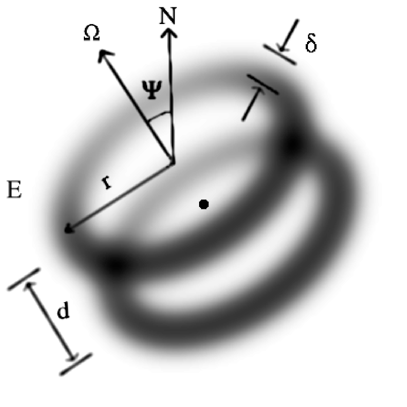
In Paper I, we developed a generic torus fitting procedure to capture the characteristic structure of PWNe. Here we give a brief summary of the model: consider a torus in 3D with radius and Gaussian cross section of thickness . The emissivity is described by
where is the direction along the torus axis and the observer line of slight lies in the -plane. As the post-shock flow in the PWNe is expected to be mildly relativistic, the torus intensity in the observer’s frame is Doppler boosted by
Here we assume a constant flow speed = radially from the pulsar in the equatorial plane. Of course this does not capture the complex latitudinal structure and speed variations seen in the MHD simulations (e.g. Del Zanna et al., 2006), but it does give a characteristic speed and captures the gross Doppler boosting. During the fitting we leave as a free parameter, but assume a fixed photon spectral index in the rest frame, which is a typical value for PWNe. We have also tried other values of , e.g. and as reported for the Vela and Crab pulsars respectively (Kargaltsev & Pavlov, 2004; Mori et al., 2004). The geometrical parameters are quite insensitive to . The phenomenological speed is slightly affected (with ), so large spectral index variations could induce trends in the fit speed. Altogether this gives
where is the total number of counts in the torus and is the inclination of the torus.
In order to compare with data, the 3-D torus is projected onto the sky plane. We set up the coordinate system for the image plane with along celestial north, along the observer line of sight and the CCD in the -plane. Then the transformation between the frames is given by
where is the position angle (N through E) of the projected torus axis. The counts in each CCD pixel (x,y) result from the integration of emissivity through the line of sight
The basic torus model is characterized by the parameters , , , and . In addition, a point source and constant background are also included in the fit. The counts in each component are determined by the fit, while the total counts in the model is constrained to match the image counts. In a few cases where twin tori are observed, there is an extra fitting parameter for the separation. For simplicity we assume a symmetrical offset along the torus axis, with the pulsar in the middle. A few other cases have inner and outer tori, at different .
To estimate the goodness of fit for particular model parameters, a likelihood function is defined using Poisson statistics. The probability of observing counts out of the expected counts in pixel is given by
In the high-count limit, we switch to Gaussian statistics for , hence the likelihood function passes to the usual statistics. The best-fit parameters are then determined by the maximum likelihood method, i.e. minimization of the Figure-of-merit function, which is defined as the negative log of the likelihood function summed over all image pixels.
Once the best-fit parameters are obtained, statistical errors in the fit are estimated by Monte Carlo simulations. Poisson realizations of the best-fit model are simulated and fitted, and the confidence interval of each parameter is obtained from their distributions. To estimate the systematic errors, we blank out different regions in the data (i.e. omit those pixels from the fit), then re-fit the model by varying only one parameter at a time while fixing the others at their best-fit values. The changes in the best-fit parameter values thus provide estimates of the uncertainties contributed by un-modeled features in the data. Note that in addition to the single parameter systemetic errors computed here, covariance between the parameters could also lead to larger errors (e.g. the covariance of with ).
2.2 Implementation
In this study we went through the CXO data archive and identified a list of observations with apparent toroidal termination shocks in PWNe (Table 1). There are a few other objects with jets and/or possible tori (e.g. PSR B150958), but for these cases closer examinations suggest that the pulsar motions maybe trans- or super-sonic with respect to the surrounding medium, hence static torus fits are not appropriate. The data are cleaned up with standard reduction procedures using CIAO and the background light curves are examined to filter out periods that suffered from strong particle flares. Then we remove the pixel randomization for the ACIS observations and apply an algorithm by Mori et al. (2001), which corrects the positions of the split pixel events, to improve the spatial resolution. Finally we select the appropriate energy range and binning to optimize the S/N of the PWNe, separating out the soft background from the SNR and field stars. To model the point source, a high S/N PSF model is simulated with the Chandra Ray Tracer (ChaRT) at the detector source position, using the source spectrum reported in literature.
| Pulsar | SNR | ObsID | Instrument | Exposure (ks) |
|---|---|---|---|---|
| J0205+6449 | 3C 58 | 3832 (catalog ADS/Sa.CXO#obs/3832), 4382 (catalog ADS/Sa.CXO#obs/4382), 4383 (catalog ADS/Sa.CXO#obs/4383) | ACIS | 350 |
| J05376910 | N157B | 2783 (catalog ADS/Sa.CXO#obs/2783) | ACIS | 50 |
| B054069 | SNR 054069.3 | 132 (catalog ADS/Sa.CXO#obs/132), 1735 (catalog ADS/Sa.CXO#obs/1735), 1736 (catalog ADS/Sa.CXO#obs/1736), 1727 (catalog ADS/Sa.CXO#obs/1727), 1738 (catalog ADS/Sa.CXO#obs/1738), 1741 (catalog ADS/Sa.CXO#obs/1741), 1745 (catalog ADS/Sa.CXO#obs/1745) | HRC | 75 |
| J11245916 | G292.0+1.8 | 1953 (catalog ADS/Sa.CXO#obs/1953) | HRC | 50 |
| B180021 | 5590 (catalog ADS/Sa.CXO#obs/5590) | ACIS | 30 | |
| J18331034 | G21.50.9 | 1230 (catalog ADS/Sa.CXO#obs/1230), 1554 (catalog ADS/Sa.CXO#obs/1554),159 (catalog ADS/Sa.CXO#obs/159), 2873 (catalog ADS/Sa.CXO#obs/2873),3700 (catalog ADS/Sa.CXO#obs/3700) | ACIS | 56 |
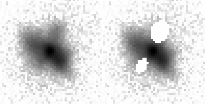
In the fitting procedure, a simulated annealing package (Press et al., 1992) is employed for multidimensional minimization of the Figure-of-merit function, with the initial parameters chosen by eye. After the best-fit model is obtained, we simulate 500 Monte Carlo Poisson realizations and estimate the statistical errors from the parameter distributions accordingly. The confidence interval, which corresponds to 68% confidence level, are reported. To estimate the systematic errors, we begin by blanking out the jet regions in the observations, since they are the most obvious un-modeled features and are present in many systems. As an example, the image of PSR B054069 with jet regions removed is shown in Figure 2. The golden section search in one dimension (Press et al., 1992) is then employed for re-fitting the model. This procedure gives systematic error estimates for the Crab, Vela (catalog ), PSRs J2229+6113 (catalog ), B170644 (catalog ), J2021+3651 (catalog ) and B054069 (catalog ). However for PSRs J1930+1852 (catalog ) and J0205+6449 (catalog ), the jets are relatively faint and well-separated from the PWNe. Therefore, removing the jets alone does not change the parameter values significantly. We believe this underestimates the systematic errors and contributions from other un-modeled features should also be considered. Therefore, we obtained another estimate by removing the point source in the data. The results reported for these two objects are the combination of the two systematic error estimates, added in quadrature.
2.3 Individual Objects
In the following we discuss the fits of some individual objects.
PSR B054069: The combined HRC exposure shows polar jet structure in the PWN. In addition, a bright blob SW of the point source is also observed. We have tried blanking out the blob in the fit, and found that the result is insensitive.
PSR J0205+6449: Similar to the Crab pulsar, a double tori structure is observed in this PWN. However, in this case the outer torus is very diffuse and without a clear boundary. In order to have a better constraint in the position angle, we fit the two tori simultaneously with the same value of .
PSR J11245916: (catalog ) While the PWN image in the initial CXO HRC observation showed noticeable ellipticity (Hughes et al., 2003), the elongation was not clear in a subsequent ACIS exposure. This could possibly due to the large off-axis angle degrading the PSF. Therefore in this study we fitted the HRC image only. A scheduled deep ACIS observation could help to resolve this structure.
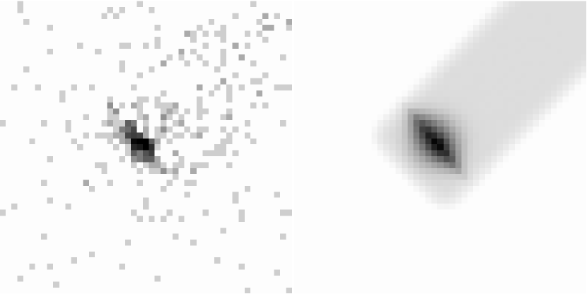
PSR J05376910: (catalog ) A cometary trail is observed in this PWN system (Chen et al., 2006), which is modeled in the fit by a rectangular background region with constant brightness. Comparison with the best-fit parameters without the background provides an estimate for the systematic errors.
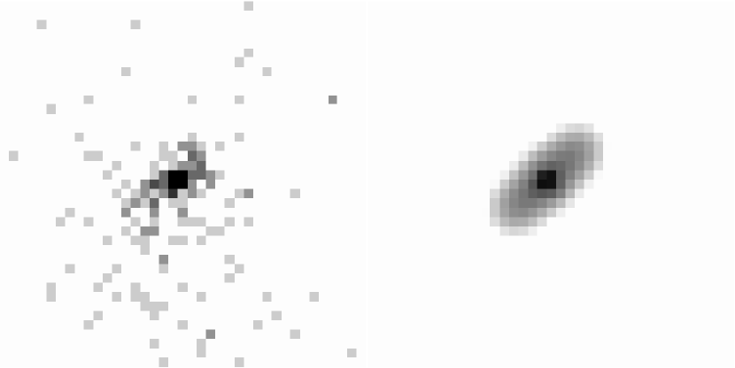
PSR B180021: (catalog ) Although the 30 ks ACIS exposure only detects a total of 200 counts (0.8-6 keV) for the point source and the PWN, the latter clearly shows extended structure with a well-defined symmetry axis. Interestingly, the direction of elongation is in general orthogonal to the proper motion claimed in Brisken et al. (2006). Hence, employing the torus fitting to obtain a quantitative measurement of the accuracy is valuable.
PSR J18331034: (catalog ) As it’s host SNR is one of the calibration objects for CXO, the pulsar has been observed repeatedly. We combined all the on-axis and in-focus ACIS observations in the data archive and obtain a total exposure of 56 ks.
PSR J05382817: In a short 20 ks ACIS exposure, diffuse emission around the pulsar was fit to a simple equatorial flow. However, while a deeper 100 ks observation (Ng et al., 2007) showed extended emission along a similar axis, it was not unambiguously possible to decide whether this was an edge-on equatorial torus or a polar jet. To be conservative, we do not include this object in the present analysis.
3 Results and Discussions
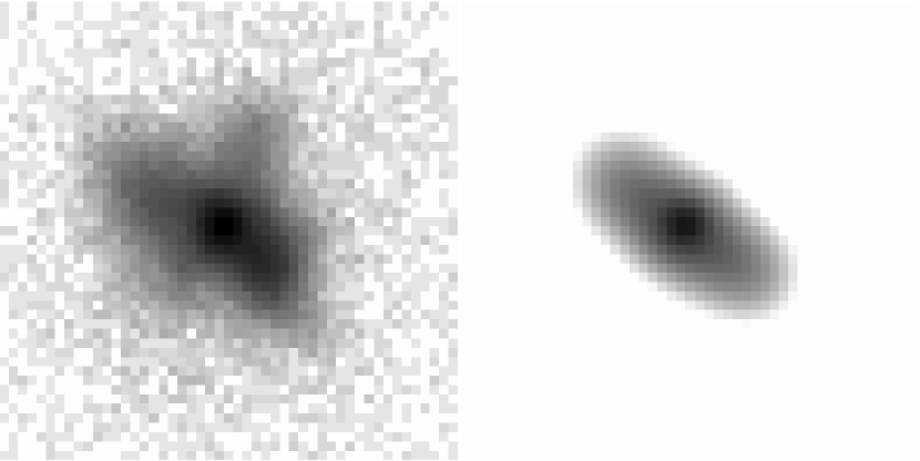
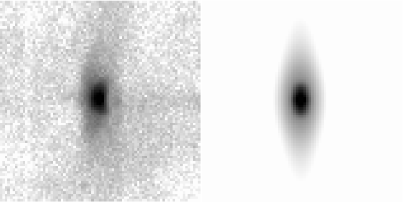
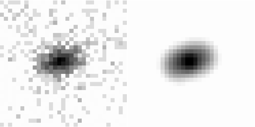
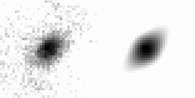
Table 3 lists the best-fit results with corresponding statistical and systematic errors. We report the systematic errors for and the separation only, since they are the most interesting parameters. Systematic errors in other parameters have similar fractional values when compared to the best-fit parameters. Note that for the faint objects, including PSRs J11245916, B180021 and J18331034, the detailed structures are not resolved and the large statistical errors dominate over the systematic errors. Therefore only the former are reported here. The best-fit models for the new objects in this study are shown in Figure 3, the rest may be found in Paper I, Figure 2 and the references listed in Table 3.
| object | sep () | PS/torus (Cts) | Ref. | |||||
|---|---|---|---|---|---|---|---|---|
| Crab (inner) | 1.5* | / | 1 | |||||
| Crab (outer) | 5.9* | / | 1 | |||||
| Vela | 3.0* | / | 1 | |||||
| J1930+1852 | 1701/602 | 1 | ||||||
| J2229+6114 | 2.5* | 2221/1113 | 1 | |||||
| B170644 | 1.0* | 2897/1221 | 2 | |||||
| J2021+3651 | 1.2* | 235/751 | 3 | |||||
| J0205+6449 (inner) | 0.74* | 5080/39730 | 4 | |||||
| J0205+6449 (outer) | 2.0* | 5080/29503 | 4 | |||||
| J05376910 | 102/179 | 4 | ||||||
| B054069 | 0.66* | 13442/50215 | 4 | |||||
| J11245916 | 390/552 | 4 | ||||||
| B180021 | 0.74* | 18/88 | 4 | |||||
| J18331034 | 304/6541 | 4 |
As shown in the table, the fits for Crab and Vela are dominated by systematic errors and the statistical errors are negligible. For the other objects, the two are comparable in and , but the systematic errors for are in general much larger. This suggests the fit is most robust in obtaining and , as they are largely determined by the shape of the torus. On the other hand, depends sensitively on the relative brightness of both sides of the torus; thus, removing the jet structure can change the results significantly.
3.1 Pulsar Jets
As mentioned in the previous section, polar jets are observed in many of the pulsars in this study. In general, the jets’ position angle is in reasonable agreement with axis determined from the torus geometry. Since these are also relativistic, relative Doppler boosting could in principle provide a second estimate of spin inclination and flow speed . However, two effects complicate this. First, might be quite different in the jets as suggested in the MHD simulations (Del Zanna et al., 2006). Second, the jets are in several cases distinctly curved, and repeated exposures of Crab and Vela indicate that this bending in the plane of the sky changes with time. Since we expect similar curvature along the line-of-sight, and even quite small changes in inclination strongly affect the brightness ratios, interpretation of the jet boosting is more difficult than that of the tori.
3.2 Pulsar Kick Connection
One direct application of the torus fitting is measurement of the neutron star’s spin axis orientation. The alignment angle between the pulsar spin and velocity vectors provides insights into the supernova core collapse physics. For a simple picture of a kick acting at a fixed spot on the neutron star surface, a longer kick duration gives a better alignment as a result of rotational averaging. Ng & Romani (2007) performed simulations of neutrino kick models and extracted constraints on the physics parameters including the kick direction, magnitude and timescale by comparing torus fitting angles with proper motion estimates and other pulsar data. As the sample of X-ray PWNe with modeled torus structure increases, the statistical constraints on such kick models should rapidly improve.
3.3 Radio Polarization
There are a few objects in our list which also have independent estimates for the spin geometry from radio polarimetry. Johnston et al. (2005), in particular, have recently made considerable progress in measuring by determining the polarization at the phase of closest approach to the magnetic pole and correcting for Faraday rotation to obtain the absolute position angle on the sky. Unfortunately, radio pulsar emission is complex and can switch between orthogonal modes; this implies a ambiguity in the spin axis orientation. Nevertheless, careful analysis can give useful position angles. At present only three of our pulsars have a from radio measurements. Johnston et al. (2005) observed the radio polarization for the Vela pulsar and obtain a P.A. of . For PSR B170644, the result is controversial: while Wang et al. (2006) report a P.A. of , Johnston et al. (2005) do not give a value, since in new observations the phase of closest approach is difficult to locate. Finally, Kothes, Reich & Uyaniker (2006) measure the radio polarization of the PWN in PSR J2229+6114 and suggest a symmetry axis at P.A.. While these three values are in reasonable agreement with the from the X-ray symmetry axis, more data are needed for a serious comparison.
Unfortunately, interpretation of the polarimetry appears to be particularly challenging for the young pulsars showing X-ray tori (this may be related to their powerful accelerators in relatively small magnetospheres). For example, the main radio pulses in the Crab appear at the same phases as the high energy emission and may indicate high-altitude emission. A classic polarization sweep may only be found for the ‘precursor’, a low frequency component. However, measurement of radio polarization for more objects would be very useful. Comparison with the X-ray P.A.s can reveal orthogonal emission in the radio, e.g. Helfand, Gotthelf & Halpern (2001), and may help to calibrate the radio polarization techniques, which may then be applied to older pulsars. PSRs J20203651 and B180021 seem amenable to such analysis.
In principle, for a simple dipole geometry it is also possible to measure the magnetic pole impact parameter (from the polarization PA sweep rate at closest approach) and the magnetic inclination (from the overall shape of the polarization position angle sweep), when the polarization is well measured over a large range of pulsar phase. In practice, while can be fairly well determined, the estimates are often poor and subject to large systematic errors. The Rotating Vector Model (RVM) for such fits was developed for Vela, so not surprisingly there are angles for this pulsar. Table 3 gives the values from Johnston et al. (2005). However, the sum is in poor agreement with the X-ray inclination of . It is difficult to interpret the CXO arc structure seen for Vela with such a small inclination. Perhaps the best approach is to adopt from the PWN structure, when available, and from radio polarization. For Vela this would imply .
3.4 The -ray Connection
Radio (coherent emission) pulse profiles are often quite complex, and may depend on the dense plasma and complex field structure at their relatively low emission altitudes. High energy (incoherent emission) profiles should be simpler, especially if they originate at high altitude where only dipole field components are expected to persist. Romani & Yadigaroglu (1995) found that for the generic class of outer magnetosphere models, the -ray pulse is usually a double peak, with a peak separation and phase lag from the radio pulse primarily determined by , although the actual values do depend on and the gap width, as well. Other models, employing emission from both hemispheres (e.g. Dyks & Rudak, 2003) can have more complex light curves with different phase relationships. However, there are some generic predictions of these models: -ray peaks are strong and wide when , they converge as approaches , and are weak or absent for small angles.
In Table 3, we list the observed GeV pulse widths () for Crab, Vela and PSR B170644 and tentative widths for two other pulsars discovered after the end of the EGRET mission. The final column () lists approximate high energy pulse widths (or ranges) from the contours in Romani & Yadigaroglu (1995), figure 4. In most cases, a range is allowed – independent (e.g. radio) values for would make width predictions. Note that for Crab and Vela, this model tends to predict somewhat narrower pulses than those seen. Also the tentative detection of PSR J2229+6114 has a wider pulse than predicted for its small . These larger angles may be easier to accommodate in two-pole models. At present there is sufficient latitude in the model predictions to allow a wide range of pulse shapes. However, new -ray observations with AGILE and, especially, GLAST should provide many high quality pulse profiles. We expect to have X-ray measurements of for many of these young pulsars. If radio observations can supply , the geometry is determined and comparison with the -ray data can powerfully refine (or eliminate) the magnetosphere models.
| Pulsar | |||||||
|---|---|---|---|---|---|---|---|
| Crab | 124 | 61 | ? | 0.39 | 0-0.35 | ||
| Vela | 131 | 64 | 137 (43)aaJohnston et al. (2005) | -6.5 | 0.42 | 0.35-0.4 | |
| J1930+1852 | 91 | 147 | 0 | ||||
| J2229+6114 | 103 | 46 | †† – fitted simultaneously. | (0.4)bbThompson et al. (2002) | |||
| B170644 | 164 | 53 | 0.25 | 0-0.3 | |||
| J2021+3651 | 45 | 79 | (0.5)ccMcLaughlin & Cordes (2003) | 0-0.45 | |||
| J0205+6449 | 90 | 92 | 0-0.55 | ||||
| J05376910 | 131 | 93 | 0-0.55 | ||||
| B054069 | 144 | 93 | 0-0.55 | ||||
| J11245916 | 16 | 105 | 0-0.45 | ||||
| B180021 | 44 | 90 | ddSmits et al. (2006) | 0.5 | |||
| J18331034 | 45 | 85 | 0-0.55 |
4 Conclusion
In conclusion, we have applied the torus fitting technique to more PWN observations in the Chandra data archive and characterized the uncertainties in the fits. This study provides a better understanding of the systematic errors, giving quantitative estimates of the measurement uncertainties. We argue that these robust position angle and inclination values are particularly useful for comparison with the radio and high energy pulse data. If new observations can fill in more measurements from these energy bands in Table 3, we should be able to make substantial progress in understanding the emission zones and viewing geometries of young pulsars.
References
- Brisken et al. (2006) Brisken, W. F., Carrillo-Barragán, M., Kurtz, S., & Finley, J. P. 2006, ApJ, 652, 554
- Chen et al. (2006) Chen, Y., Wang, Q. D., Gotthelf, E. V., Jiang, B., Chu, Y.-H., & Gruendl, R. 2006, ApJ, 651, 237
- Del Zanna et al. (2006) Del Zanna, L., Volpi, D., Amato, E., & Bucciantini, N 2006 A&A, 453, 621
- Dyks & Rudak (2003) Dyks, J., & Rudak, B. 2003, ApJ, 598, 1201
- Helfand, Gotthelf & Halpern (2001) Helfand D. J., Gotthelf E. V., Halpern J. P. 2001, ApJ, 556, 380
- Hessels et al. (2004) Hessels, J. W. T., Roberts, M. S. E., Ransom, S. M., Kaspi, V. M., Romani, R. W., Ng, C.-Y., Freire, P. C. C., Gaensler, B. M. 2004, ApJ, 612, 389
- Hughes et al. (2003) Hughes, J. P., Slane, P. O., Park, S., Roming, P. W. A., & Burrows, D. N. 2003, ApJ, 591, L139
- Johnston et al. (2005) Johnston, S., Hobbs, G., Vigeland, S., Kramer, M., Weisberg, J. M., & Lyne, A. G. 2005, MNRAS, 364, 1397
- Kothes, Reich & Uyaniker (2006) Kothes, R., Reich, W., & Uyaniker, B. 2006, ApJ, 638, 225
- Kargaltsev & Pavlov (2004) Kargaltsev, O., & Pavlov, G. G. 2004, in ASP Conf. Ser. 218, Young Neutron Stars and Their Environments, ed. F. Camilo & B. M. Gaensler (San Francisco: ASP), 195
- Komissarov & Lyubarsky (2003) Komissarov, S. S., & Lyubarsky, Y. E. 2003, MNRAS, 344, L93
- McLaughlin & Cordes (2003) McLaughlin, M. A., & Cordes, J. M. 2003, in Proceedings of The Fourth AGILE Science Workshop on “X-ray and Gamma-ray Astrophysics of Galactic Sources”, ed. W. Collmar (Rome: AGILE)
- Mori et al. (2001) Mori, K., Tsunemi, H., Miyata, E., Baluta, C. J., Burrows, D. N., Garmire, G. P., & Chartas, G. 2001, in ASP Conf. Ser. 251, New Century of X-Ray Astronomy, ed. H. Inoue & H. Kunieda (San Francisco: ASP), 576
- Mori et al. (2004) Mori, K., et al. 2004, ApJ, 609, 186
- Ng & Romani (2004) Ng, C.-Y., & Romani, R. W. 2004, ApJ, 601, 479 (Paper I)
- Ng & Romani (2007) Ng, C.-Y., & Romani, R. W. 2007, ApJ, 660, 1357
- Ng et al. (2007) Ng, C.-Y., Romani, R. W., Brisken, W. F., Chatterjee, S., & Kramer, M. 2007, ApJ, 654, 487
- Rees & Gunn (1974) Rees, M. J., & Gunn, J. E. 1974, MNRAS, 167, 1
- Romani et al. (2004) Romani, R. W., & Ng, C.-Y. 2004, ApJ, 585, L41
- Romani et al. (2005) Romani, R. W., Ng, C.-Y., Dodson, R., & Brisken, W. 2005, ApJ, 631, 480
- Romani & Yadigaroglu (1995) Romani, R. W., & Yadigaroglu, I.-A. 1995, ApJ, 438, 314.
- Press et al. (1992) Press, W. H., Flannery, B. P., Teukolsky, S., & Vetterling, W. 1992, Numerical Recipes in C: The Art of Scientific Computing (Cambridge: Cambridge Univ. Press)
- Smits et al. (2006) Smits, J. M., Stappers, B. W., Edwards, R. T., Kuijpers, J., & Ramachandran, R. 2006, A&A, 448, 1139
- Thompson et al. (2002) Thompson, D. J., Digel, S. W., Nolan, P. L., & Reimer, O. 2002, in ASP Conf. Ser. 271, Neutron Stars in Supernova Remnants, ed. P. O. Slane & B. M. Gaensler (San Francisco: ASP), 65
- Wang et al. (2006) Wang, C., Lai, D., & Han, J. L. 2006, ApJ, 639, 1007
- Weisskopf et al. (2001) Weisskopf, M. C., et al. 2000, ApJ, 536, L81