From the Entropy to the Statistical Structure
of Spike Trains

Abstract

We use statistical estimates of the entropy rate of individual spike train data in order to make inferences about the underlying structure of the spike train itself. We first examine a number of different parametric and nonparametric estimators (some known and some new), including the “plug-in” method, several versions of Lempel-Ziv-based compression algorithms, a maximum likelihood estimator tailored to renewal processes, and the natural estimator derived from the Context-Tree Weighting method (CTW). The theoretical properties of these estimators are examined, several new theoretical results are developed, and all estimators are systematically applied to various types of simulated data under different conditions.

Our main focus is on the performance of these entropy estimators on the (binary) spike trains of 28 neurons recorded simultaneously for a one-hour period from the primary motor and dorsal premotor cortices of a monkey. We show how the entropy estimates can be used to test for the existence of long-term structure in the data, and we construct a hypothesis test for whether the renewal process model is appropriate for these spike trains. Further, by applying the CTW algorithm we derive the maximum a posterior (MAP) tree model of our empirical data, and comment on the underlying structure it reveals.

I Introduction

Information-theoretic methods have been widely used in neuroscience, in the broad effort to analyze and understand the fundamental information-processing tasks performed by the brain. In these studies, the entropy has been adopted as a central measure for quantifying the amount of information transmitted between neurons. One of the most basic goals is to identify appropriate methods that can be used to estimate the entropy of spike trains recorded from live animals.

The most commonly used entropy-estimation technique is probably the so-called “plug-in” (or maximum-likelihood) estimator and its various modifications. This method consists of essentially calculating the empirical frequencies of all words of a fixed length in the data, and then estimating the entropy rate of the data by calculating the entropy of this empirical distribution; see, e.g., [14][9][16][10][13][8][2]. For computational reasons, the plug-in estimator cannot go beyond word-lengths of about 10 or 20, and hence it does not take into account the potential longer time dependence in the signal.

Here we examine the performance of various entropy estimators, including some based on the Lempel-Ziv (LZ) data compression algorithm [19], and some based on the Context-Tree Weighting (CTW) method for data compression. We employed four different LZ-based methods; of those, two [5], have been widely and very successfully used in many applications (e.g., [12][5]), and the other two are new estimators with some novel and more desirable statistical properties. The CTW-based estimator we used is based on the results in [17][18] and it has also been considered in [4][6].

We demonstrate that the LZ- and CTW-based estimators naturally incorporate dependencies in the data at much longer time scales, and that they are consistent (in the statistical sense) for a wide class of data types generated from distributions that may possess arbitrarily long memory.

To compare the performance of various methods, we applied these entropy estimators on simulated data generated from a variety of different processes, with varying degrees of dependence. We study the convergence rate of the bias and variance of each estimator, and their relative performance in connection with the length of the memory present in the data.

Finally, we applied these methods to neural data, recorded from two multi-electrode arrays implanted on a monkey’s primary motor cortex (MI) and dorsal premotor cortex (PMd). The arrays simultaneously recorded neural activity from 28 different neurons. A Plexon acquisition system was used to collect neural signal, and the units were spike-sorted using Plexon’s Offline Sorter. The monkey was not engaged in any task when the data were collected, and the size of the data is approximately an hour. A detailed description of recording techniques is given in [7].

Our main conclusions can be summarized as follows:

$\bullet\;$ The CTW was consistently the most reliable and accurate estimator.

$\bullet\;$ The results of the CTW compared with those of the plug-in method very strongly suggest that there are significant longer-term dependencies in the data.

$\bullet\;$ One of the most significant features of our results is the observation that from the CTW algorithm we can also obtain an explicit statistical model for the data, the so-called maximum a posteriori probability tree model [15]. From the resulting tree structures we deduce several interesting aspects of spike train patterns. In particular, we find that the primary statistical feature of a spike train captured by the CTW estimator is its empirical inter-symbol interval (ISI) distribution.

$\bullet\;$ Among all the estimators we considered, the CTW with large depth $D$ is the only method able to capture the longer term statistical structure of renewal data with ISI distribution that is close to that of real neurons.

$\bullet\;$ The spike train data we examined can, to a statistically significant degree of accuracy, be modelled as renewal processes with independent ISIs. Specifically, in the entropy estimation task, among the various sources of bias, the bias incurred by treating the spike train as a renewal process is negligible for the neurons considered.

$\bullet\;$ In our entropy estimation experiments on spike trains we generally observed that, as the tree depth of the CTW increases, the corresponding entropy estimates decrease. This decrease is significantly larger than would be expected from purely random fluctuations, if there was actually no long-term structure in the data.

$\bullet\;$ The percentage of drop is correlated with the variability of the spike count in the data (as quantified by the Fano factor). This conclusion is rigorously justified with a $t$-test with a $p$-value of $\approx 5\times 10^{-4}$. Perhaps most interestingly, since the test was done on data in 100ms windows, it implies that the correlation is not simply due to refractoriness or any other structure that appears on a fine time scale.

II Experimental Results and Findings

Our neuronal data come from binned spike trains recorded simultaneously from 28 neurons, with bin size equal to 1ms. The total length of each spike train is $N=3,606,073$ms, which is a little over an hour. Five out of the 28 neurons have average firing rates lower than 1Hz, 16 are between 1Hz and 10Hz, 6 are between 11Hz and 20Hz, and one has a firing rate above 20Hz. Figure 1 shows the autocorrelograms for 12 of the 28 neurons and the empirical inter-symbol interval (ISI) distributions for 4 of the 28 neurons. These plots show that there is great richness and variability in the statistical behavior of different neurons.

Figure 1: The first three rows show the autocorrelograms of 12 out of the 28 spike trains from 28 different neurons. Lag varies from -300ms to 300ms. The last row shows the empirical ISI distributions of 4 spike trains from 4 of the 28 neurons. ISI values vary from zero to 1000ms.

II-A Entropy Estimates

Figure 2 shows the results of estimating the entropy rate of these spike trains, using the plug-in method, two LZ estimators, and the CTW algorithm.

Figure 2: Entropy estimates obtained by several methods, shown in bits-per-ms and plotted against the mean firing rate of each neuron. The purple curve is the entropy rate of an i.i.d. process with the corresponding firing rate. The results of the plug-in (with word-length $20$) are shown as black x’s; the results of the two LZ-based estimators as red circles and blue triangles; and the results of the CTW method as green squares.

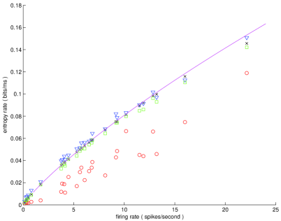
Note that all the estimates generally increase as the firing rate goes up, and that the i.i.d. curve corresponds exactly to the value to which the plug-in estimator with word length $1$ms would converge with infinitely long data. The plug-in estimates with word length $20$ms are slightly below the i.i.d. curve, and the CTW estimates tend to be slightly lower than those of the plug-in. It is important to observe that, although the bias of the plug-in is negative and the bias of the CTW is positive, we consistently find that the CTW estimates are smaller than those of the plug-in. This strongly suggests that the CTW does indeed find significant longer-term dependencies in the data.

For the two LZ estimators, we observe that one gives results that are systematically higher than those of the plug-in, and the other is systematically much lower. The main limitation of the plug-in is that it can only use words of length up to 20ms, and even for word lengths around 20ms the undersampling problem makes these estimates unstable. Moreover, this method completely misses the effects of longer term dependence. Several ad hoc remedies for this drawback have been proposed in the literature; see, e.g., [14].

The main drawback of the LZ estimators is the slow rate of convergence of their bias, which is relatively high and hard to evaluate analytically.

As we found in extensive simulation studies, the bias of the CTW estimator converges much faster than the biases of the LZ estimators, while keeping the advantage of dealing with long-range dependence. Moreover, from the CTW we can obtain an explicit statistical model for the data, the “maximum a posteriori probability” (MAP) tree described in [15]. The importance of these models comes from the fact that, in the information-theoretic context, they can be operationally interpreted as the “best” tree models for the data at hand.

II-B MAP Tree Models for Spike Trains

We computed the MAP tree models [15] derived from spike train data using the CTW algorithm with depth $D=100$. Figure 3 shows the suffix sets of two cells’ MAP trees, sorted in descending order of suffix frequency. The most frequent suffix is always the all-zero suffix, generally followed by suffixes of the form “$1000000\cdots 0$.” Similarly to the results of Figure 1, we find a lot of variability between neurons.

Figure 3: Suffix sets of MAP trees derived from the spike trains of cells 1 and 4, whose mean rates are 4.15Hz and 6.52Hz, respectively. Suffixes are sorted in descending order of frequency. The green areas are zeros in the suffixes, red dots are 1’s, and the blue areas mark the end of each suffix.

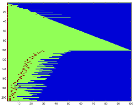
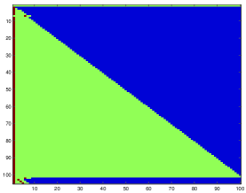
Since suffixes of the form “$100\cdots 0$” are the most common non-zero suffixes produced by the CTW, we note that in 22 out of the 28 neurons the percentage of such suffixes among all the non-zero suffixes in the MAP trees we obtained exceeds 75%. Since the frequency of each such suffix is exactly the same as the frequency of an inter-spike interval with the same length, we interpret the high frequency of “$100\cdots 0$” suffixes as an indication that the primary statistical feature of a spike train captured by the CTW estimator is its empirical inter-symbol interval (ISI) distribution.

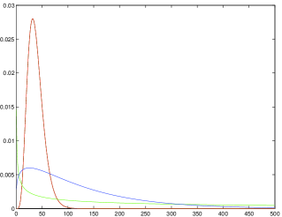
This observation motivates us to look at renewal process models in more detail. Next we examine the performance of different entropy estimators on simulated data from renewal processes whose ISI distribution is close to that of real spike trains. For that, we first estimate the ISI distribution of our spike trains. Using the empirical ISI distribution is problematic since such estimates are typically undersampled and hence unstable. Instead, we developed and used a simple iterative method to fit a mixture of three Gamma’s to the empirical estimate. The idea is based on the celebrated EM algorithm [3]. The components of the mixtures can be though of as capturing different aspects of the ISI distribution of real neurons. For cell no. 1, for example, Figure 4 shows the shapes of these three components. One of them is highly peaked around 40ms, probably due to refractoriness; another component appears to take into account longer-range dependence, and the last component adjusts some details of the shape.

Figure 4: The three components of the mixture of Gamma’s fitted to cell 1.

We then run various estimators on simulated data from renewal processes with ISI distributions given by the three-Gamma mixtures obtained from the spike train data. Figure 5 shows the bias of various estimators as a percentage of the true entropy rate, for simulated data with ISI distributions given by the Gamma-mixtures obtained from cell 1. The data lengths are $N=5000$, $10^{4}$, $10^{5}$ and $10^{6}$.

Figure 5: Bias (as a percentage of true entropy rate) of various entropy estimators applied to simulated data from a renewal process with ISI distribution given by a mixture of Gammas fitted to the spike train of neuron no. 1. The data lengths are $N=5000$, $10^{4}$, $10^{5}$ and $10^{6}$, and the $x$-axis is $\log_{10}N$. The upper and lower dotted lines represent two standard deviations away from the true values, where the standard deviation is obtained as the average of the standard errors of all the methods. The plug-in has word-length $20$ms, and the CTW estimator is used with four different tree depths, $D=10,20,50,100.$ The true entropy rate of this “cell” is 0.0347 bits/ms.

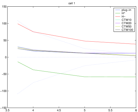
As we can see from the plot, the LZ estimators converge very slowly, while the plug-in and CTW estimates are much more accurate. The estimates obtained by the plug-in with word-length $20$ms and by the CTW with depths $D$=10, 20 are very similar, as we would expect. But for data sizes $N=10^{5}$ or greater, the CTW with longer depth gives significantly more accurate results that outperform all other methods. Similar comments apply to the results for most other cells, and for some cells the difference is even greater in that the CTW with depth $D=20$ already significantly outperforms the plug-in with the same word length. The standard error of the plug-in and the CTW estimates is larger than their bias for small data lengths, but at $N=10^{6}$ the reverse happens.

In short, we find that that the CTW with large depth $D$ is the only method able to capture the longer term statistical structure of renewal data with ISI distribution that is close to that of real neurons. For cell no. 1, for example, the largest ISI value in the data is 15.7 seconds. Therefore, there is significant structure at a scale that is much greater that the plug-in window of 20ms, and the CTW apparently can take advantage of this structure to improve performance.

Finally, we remark on how the choice of the depth $D$ affects the CTW estimator; a more detailed discussion is given in Section II-D below. For smaller data sizes $N$, the results of the CTW with $D=10$ are very close to those with $D=100$, but for $N=10^{5}$ and $N=10^{6}$ the difference becomes quite significant. This is likely due to the fact that, for small $N$, there are not enough long samples to represent the long memory of the renewal processes, and the estimation bias is dominated by the undersampling bias. For large $N$, on the other hand, undersampling problems become more minor, and the difference produced by the longer-term dependence captured by larger depths becomes more pronounced.

II-C Testing the Non-renewal Structure of Spike Trains

The above results, both on simulated data and on real neural data, strongly indicate that the CTW with large tree depth $D$ is the best candidate for accurately estimating the entropy rate of binned spike trains. They also suggest that the main statistical pattern captured in the CTW’s estimation process is the renewal structure that seems to be inherently present in our data. It is then natural to ask how accurately a real spike train can be modelled as renewal process, or, equivalently, how much is “lost” if we assume that the data are generated by a renewal process.

Recall that, if a spike train has dependent ISIs, then its entropy rate will be lower than that of a renewal process with the same ISI distribution. Therefore we can specifically ask the following question: If we took the data corresponding to a real spike train and ignored any potential dependence in the ISIs, would the estimated entropy differ significantly from the corresponding estimates using the original data?

To answer the above questions we performed the following experiment. For a given neuron, we estimated the ISI distribution by a three-Gamma mixture as described earlier and generated a renewal process with that ISI distribution. Then we randomly selected long segments of fixed length from the simulated data and estimated the entropy using the CTW algorithm with depth $D=100$; the same was done with the real spike train. Finally, we compared the average value of the estimates from the simulated data set to that of the spike train estimates. We used 100 segments from each data set, of lengths $N=1000$, $10^{4}$, $10^{5}$ and $10^{6}$. Figure 6 shows the difference between the two (averaged) estimates, that is, the estimated entropy of the real spike train minus the estimated entropy of the corresponding renewal process. We also plot error bars corresponding to two standard deviations of this difference. The same experiment was performed on data from three different cells.

Figure 6: Difference of entropy estimates on spike trains and on simulated data from a renewal process with the same ISI distribution. The segment lengths are $N=10^{3}$,$10^{4}$, $10^{5}$, and $10^{6}$. The $x$-axis is $\log_{10}{N}$ and the $y$-axis is the difference between the estimates in bits/ms. For each $N$, a hundred randomly chosen segments from real data (and the same number of realizations of simulated data) are used to compute the estimates, using the CTW algorithm with $D=100$. The difference is the average of the 100 estimates based on real data minus the corresponding average on simulated data. The error bar is two standard deviations of the estimated difference.

From the plots we can see that at smaller $N$ the error bars are very wide and the estimated difference well within two standard deviations away from zero. Even at $N=10^{6}$ where the difference becomes more apparent, it remains very close to the two-standard-deviation bound. Hence the results suggest that either there is no significant difference, or, if it exists, it is rather negligible. In other words, among the various sources of bias in the entropy estimation process (such as CTW’s inherent upward bias, the negative bias due to undersampling, and so on), the bias incurred by treating the spike train as a renewal process is negligible for the neurons we examined.

II-D Memory Length in Spike Trains

A natural measure of the amount of dependence or long-term memory in a process $\{X_{n}\}$, is the rate at which the conditional entropy $H(X_{n}|X_{n-1},\ldots,X_{1})$ converges to the entropy rate $H$. We can relate this rate of decay to the tree depth of the CTW algorithm in the following way. If the data are generated from a tree source with depth $D$ (or any source with memory-length that does not exceed $D$), then the CTW estimator will converge to the true entropy rate, which, in this case, is equal to the conditional entropy, $H(X_{D+1}|X_{D},\ldots,X_{1}).$ If, on the other hand, the data comes from a process with longer memory, the estimates will still converge to $H(X_{D+1}|X_{D},\ldots,X_{1}),$ but this will be strictly larger than the actual entropy rate. Therefore, in principle, we could perform the following experiment: Given unlimited data and computational resources, we could estimate the entropy using the CTW with different tree depths $D$. As $D$ increases the estimates will decrease, up to the point where we reach the true memory length of the process, after which the estimates will remain constant. Of course in practice we are limited by the length of the data available (which adds bias and variability), and also by the amount of computation we can perform (which restricts the range of $D$’s we may consider). Nevertheless, for the case of the spike train data at hand, some conclusions can be drawn with reasonable confidence.

In our experiments on spike trains we generally observed that, as the tree depth $D$ of the CTW increases, the corresponding entropy estimates decrease; see Figure 5. However, the percentage of drop from $D=1$ to $D=100$ varies greatly from neuron to neuron, ranging from 0% to 8.89%, with a mean of 4.01% and standard deviation 2.74%. These percentages are shown as blue circles in Figure 7(a). Since it is not a priori clear whether the drop in the entropy estimates is really due to the presence of longer term structure or simply an artifact of the bias and variability of the estimation process, in order to get some measure for comparison we performed the same experiment on a memoryless process: We generated i.i.d. data with the same length and mean firing rate as each of the neurons, and computed the percentage of drop in their entropy estimates from $D=1$ to $D=100$; the corresponding results are plotted in Figure 7(a) as red crosses.

Figure 7: (a) Percentage of drop in the CTW entropy estimates from $D=1$ to $D=100$, plotted against each neuron’s firing rate. Blue circles denote the results on the 28 neural spike trains. Red crosses are corresponding results on simulated i.i.d. data with the same mean firing rates as real neurons. (b) Scatter plot of the Fano factors of real neurons (with a 100ms window) plotted against the percentage of drop in their entropy estimates.

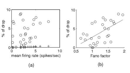
From the plots we clearly see that the drop in the entropy estimates on i.i.d. data is significantly smaller and much more uniform across neurons, compared to the corresponding results on the spike train data. We next investigate the potential reasons for this drop, and ask whether these results indicate that some neurons have more long-term structure and longer time dependency than others. An important quantity for these considerations – often used to quantify the variability of a spike train – is the Fano factor. This is defined as the ratio of the variance of the number of spikes counted in a specified time window, to the average spike count in such a window; see, e.g., [11]. Figure 7(b) shows the scatter plot of the Fano factors of real neurons (computed with a 100ms bin size) against the percentage of drop in their entropy estimates. At first glance, at least, they appear to be positively correlated. To quantify the significance of this observation we use a $t$-test: The null hypothesis is that the correlation coefficient between the Fano factors and the percentage drop is zero, and the test statistic is $t=\frac{r\sqrt{n-2}}{\sqrt{1-r^{2}}}\sim t_{n-2},$ where $r$ is the sample correlation and $n$ is the number of samples; here $r=0.5843$, $n=28$. The test gives $p$-value of $5.4802\times 10^{-4}$, which means that we can confidently reject the null, or, alternatively, that the Fano factors and the entropy drops are positively correlated.

Recall [11, pp.52-53], that the Fano factor of i.i.d. data (i.e., data from a renewal process with ISIs that are geometrically distributed, often referred to as “Poisson data”) is exactly equal to 1, whereas for most of the neurons with large percentage of drops we find Fano factors greater than 1. This is further indication that in neurons with larger percentages of drop in the entropy estimates we see greater departure from i.i.d. firing patterns. We should also note that, since the Fano factor with a 100ms bin is completely blind to anything that happens in shorter time scales, this is not a departure from i.i.d. firing in terms of the fine time structure. Among potential explanations we briefly mention the renewal structure of the data with perhaps long tails in the ISI distribution, and also the possibility of a “slow” modulation of the firing rate, creating longer memory in the data, although the latter explanation cannot explain the heavy-tailed nature of the ISIs observed.

Acknowledgments

Y.G. was supported by the Burroughs Welcome fund. I.K. was supported by a Sloan Foundation Research Fellowship and by NSF grant #0073378-CCR. E.B. was supported by NSF-ITR Grant #0113679 and NINDS Contract N01-NS-9-2322. We thank Nicho Hatsopoulos for providing the neural data set.

References

- [1]
- [2] R.R. de Ruyter van Steveninck, et. al. Reproducibility and variability in neural spike trains. Science, 275:1805–1808, 1997.
- [3] A.P. Dempster, N.M. Laird and D.B. Rubin. Maximum likelihood from incomplete data via the EM algorithm (with discussion). Journal of the Royal Stat Society B, 39:1–38, 1977.
- [4] M. Kennel and A. Mees. Context-tree modeling of observed symbolic dynamics. Phys. Rev. E, 66:056209, 2002.
- [5] I. Kontoyiannis, P.H. Algoet, Yu.M. Suhov and A.J. Wyner. Nonparametric entropy estimation for stationary processes and random fields, with applications to English text. IEEE Trans. Inform. Theory, 44:1319–1327, 1998.
- [6] M. London. The information efficacy of a synapse. Nature Neurosci., 5(4):332–340, 2002.
- [7] E. Maynard, N. Hatsopoulos, C. Ojakangas, B. Acuna, J. Sanes, R. Normann and J. Donoghue. Neuronal interaction improve cortical population coding of movement direction. J. of Neuroscience, 19(18):8083–8093, 1999.
- [8] I. Nemenman, W. Bialek and R. de Ruyter van Steveninck. Entropy and information in neural spike trains: progress on the sampling problem. Physical Review E, 056111, 2004.
- [9] L. Paninski. Estimation of entropy and mutual information. Neural Comp., 15:1191–1253, 2003.
- [10] P. Reinagel. Information theory in the brain. Current Biology, 10(15):R542–R544, 2000.
- [11] F. Rieke, D. Warland, R. de Ruyter van Steveninck and W. Bialek. Spikes, exploring the neural code. The MIT Press, 1997.
- [12] T. Schürmann and P.Grassberger. Entropy estimation of symbol sequences. Chaos, 6:414–427, 1996.
- [13] C.F. Stevens and A.Zador. Information through a spiking neuron. NIPS, 8, 1996.
- [14] S.P. Strong, R. Koberle, R. de Ruyter van Steveninck and W. Bialek. Entropy and information in neural spike trains. Physical Review Letters, 80:197–200, 1998.
- [15] P.A.J. Volf and F.M.J. Willems. On the context tree maximizing algorithm. Proceedings of the 1995 IEEE International Symposium on Information Theory, 1995.
- [16] D.K. Warland, P. Reinagel and M. Meister. Decoding visual infomation from a population of retinal ganglion cells. J. of Neurophysiology, 78(5):2336–2350, 1997.
- [17] F.M.J. Willems, Y.M. Shtarkov and T.J. Tjalkens. The Context-tree weighting method: basic properties. IEEE Trans. Inform. Theory, 41:653–664, 1995.
- [18] F.M.J. Willems. The Context-tree weighting method: extensions. IEEE Trans. Inform. Theory, 44:792–798, 1998.
- [19] J. Ziv and A. Lempel. A universal algorithm for sequential data compression. IEEE Trans. Inform. Theory, 23:337–343, 1977.