On the performance of algorithms for the minimization of $\ell_{1}$-penalized functionals

Abstract

The problem of assessing the performance of algorithms used for the minimization of an $\ell_{1}$-penalized least-squares functional, for a range of penalty parameters, is investigated. A criterion that uses the idea of ‘approximation isochrones’ is introduced. Five different iterative minimization algorithms are tested and compared, as well as two warm-start strategies. Both well-conditioned and ill-conditioned problems are used in the comparison, and the contrast between these two categories is highlighted.

1 Introduction

In recent years, applications of sparse methods in signal analysis and inverse problems have received a great deal of attention. The term compressed sensing is used to describe the ability to reconstruct a sparse signal or object from far fewer linear measurements than would be needed traditionally [1].

A promising approach, applicable to the regularization of linear inverse problems, consists of using a sparsity-promoting penalization. A particularly popular penalization of this type is the $\ell_{1}$ norm of the object in the basis or frame in which the object is assumed to be sparse. In [2] it was shown that adding an $\ell_{1}$ norm penalization to a least squares functional (see expression (1) below) regularizes ill-posed linear inverse problems . The minimizer of this functional has many components exactly equal to zero. Furthermore, the iterative soft-thresholding algorithm (IST) was shown to converge in norm to the minimizer of this functional (earlier work on $\ell_{1}$ penalties is in [3, 4]).

It has also been noted that the convergence of the IST algorithm can be rather slow in cases of practical importance, and research interest in speeding up the convergence or developing alternative algorithms is growing [5, 6, 7, 8, 9]. There are already several different algorithms for the minimization of an $\ell_{1}$ penalized functional. Therefore, it is necessary to discuss robust ways of evaluating and comparing the performance of these competing methods. The aim of this manuscript is to propose a procedure that assesses the strengths and weaknesses of these minimization algorithms for a range of penalty parameters.

Often, authors compare algorithms only for a single value of the penalty parameter and may thereby fail to deliver a complete picture of the convergence speed of the algorithms. For the reader, it is difficult to know if the parameter has been tuned to favor one or the other method. Another issue plagueing the comparison of different minimization algorithms for problem (2) below is the confusion that is made with sparse recovery. Finding a sparse solution of a linear equation and finding the minimizer of (2) are closely related but (importantly) different problems: The latter will be sparse (the higher the penalty parameter, the sparser), but the former does not necessarily minimize the $\ell_{1}$ penalized functional for any value of the penalty parameter. Contrary to many discussions in the literature, we will look at the minimization problem (2) independently of its connection to sparse recovery and compressed sensing.

The central theme of this note is the introduction of the concept of approximation isochrone, and the illustration of its use in the comparison of different minimization algorithms. It proves to be an effective tool in revealing when algorithms do well and under which circumstances they fail. As an illustration, we compare five different iterative algorithms. For this we use a strongly ill-conditioned linear inverse problem that finds its origin in a problem of seismic tomography [10], a Gaussian random matrix (i.e. the matrix elements are taken from a normal distribution) as well as two additional synthetic matrices. In the existing literature, most tests are done using only a matrix of random numbers, but we believe that it is very important to also consider other matrices. Actual inverse problems may depend on an operator with a less well-behaved spectrum or with other properties that could make the minimization more difficult. Such tests are usually not available. Here we compare four operators. Among other things, we find that the strongly singular matrices are more demanding on the algorithms.

We limit ourselves to the case of real signals, and do not consider complex variables. In this manuscript, the usual $2$-norm of a vector $x$ is denoted by $\|x\|$ and the $1$-norm is denoted by $\|x\|_{1}$. The largest singular value of a matrix $K$ is denoted by $\|K\|$.

2 Problem statement

After the introduction of a suitable basis or frame for the object and the image space, the minimization problem under study can be stated in its most basic form, without referring to any specific physical origin, as the minimization of the convex functional

$$F_{\lambda}(x)=\|Kx-y\|^{2}+2\lambda\|x\|_{1}$$ (1)

in a real vector space ($x\in\mathbb{R}^{p}$, $\lambda\geq 0$), for a fixed linear operator $K\in\mathbb{R}^{m\times p}$ and data $y\in\mathbb{R}^{m}$. In the present analysis we will assume the linear operator $K$ and the data $y$ are such that the minimizer of (1) is unique. This is a reasonable assumption as one imposes penalty terms, typically, to make the solution to an inverse problem unique.

We set

$$\bar{x}(\lambda)=\arg\min_{x}\|Kx-y\|^{2}+2\lambda\|x\|_{1}.$$ (2)

The penalty parameter $\lambda$ is positive; in applications, it has to be chosen depending on the context. Problem (2) is equivalent to the constrained minimization problem:

$$\tilde{x}(\rho)=\arg\min_{\|x\|_{1}\leq\rho}\|Kx-y\|^{2}\qquad$$ (3)

with an implicit relationship between $\rho$ and $\lambda$: $\rho=\|\bar{x}(\lambda)\|_{1}$. It follows from the equations (4) below that the inverse relationship is: $\lambda=\max_{i}|(K^{T}(y-K\tilde{x}(\rho)))_{i}|$. Under these conditions one has that: $\bar{x}(\lambda)=\tilde{x}(\rho)$. One also has that $\bar{x}(\lambda)=0$ for all $\lambda\geq\lambda_{\mathrm{max}}\equiv\max_{i}|(K^{T}y)_{i}|$.

2.1 Direct method

An important thing to note is that the minimizer $\bar{x}$ (and thus also $\tilde{x}$) can in principle be found in a finite number of steps using the homotopy/LARS method [11, 12]. This direct method starts from the variational equations which describe the minimizer $\bar{x}$:

$$\begin{array}[]{lclcl}(K^{T}(y-K\bar{x}))_{i}&=&\lambda\;\mathrm{sgn}(\bar{x}_{i})&\mathrm{if}&\bar{x}_{i}\neq 0\\ |(K^{T}(y-K\bar{x}))_{i}|&\leq&\lambda&\mathrm{if}&\bar{x}_{i}=0\end{array}$$ (4)

Because of the piece-wise linearity of the equations (4), it is possible to construct $\bar{x}(\lambda_{\mathrm{stop}})$ by letting $\lambda$ in (4) descend from $\lambda_{\mathrm{max}}$ to $\lambda_{\mathrm{stop}}$, and by solving a linear system at every value of $\lambda$ where a component in $\bar{x}(\lambda)$ goes from zero to nonzero or, exceptionally, from nonzero to zero. The first such point occurs at $\lambda=\lambda_{\mathrm{max}}$. The linear systems that have to be solved at each of these breakpoints are ‘small’, starting from $1\times 1$ and ending with $s\times s$, where $s$ is the number of nonzero components in $\bar{x}(\lambda_{\mathrm{stop}})$. Such a method thus constructs $\bar{x}(\lambda)$ exactly for all $\lambda_{\mathrm{max}}\geq\lambda\geq\lambda_{\mathrm{stop}}$, or equivalently all $\bar{x}$ with $0\leq\|\bar{x}(\lambda)\|_{1}\leq\|\bar{x}(\lambda_{\mathrm{stop}})\|_{1}$. It also follows that $\bar{x}(\lambda)$ is a piecewise linear function of $\lambda$.

Implementations of this direct algorithm exist [13, 14, 15], and exhibit a time complexity that is approximately cubic in $s$ (the number of nonzero components of $\bar{x}(\lambda)$). If one is interested in sparse recovery, this is not necessarily a problem as time complexity is linear for small $s$. In fact, the algorithm can be quite fast, certainly if one weighs in the fact that the exact minimizer (up to computer round-off) is obtained. A plot of the time complexity as a function of the number of nonzero components in $\bar{x}(\lambda)$ is given in figure 1 (left hand side) for an example operator $K^{(1)}$ and data $y$ (see start of section 4 for a description of $K^{(1)}$). The plot shows that the direct algorithm is useable in practice for about $s\leq 10^{3}$. This graph also illustrates the fact that the size of the support of $\bar{x}(\lambda)$ does not necessarily grow monotonically with decreasing penalty parameter (this depends on the operator and data).

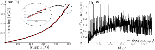
Figure 1: Left: Time complexity of the direct algorithm mentioned in section 2. Horizontal axis: number of nonzero components in the minimizer $\bar{x}$. Vertical axis: time needed by the direct algorithm to calculate this minimizer (seconds). The continuous line represents a cubic fit. The support of $\bar{x}(\lambda)$ may sometimes decrease for increasing values of $\|\bar{x}(\lambda)\|_{1}$. This phenomenon is clearly visible in the zoomed area. Right: The relative error, $\|\bar{x}-S_{\lambda}(\bar{x}+K^{T}(y-K\bar{x}))\|/\|\bar{x}\|$, of the resulting minimizer at each step (there are more steps than nonzero components because of the phenomenon in the zoomed area in the left hand side plot). Due to floating point arithmetic, this is not exactly zero. These two pictures were made by letting $\lambda$ decrease from $\lambda_{\mathrm{max}}$ to $\lambda_{\mathrm{stop}}=\lambda_{\mathrm{max}}/2^{15.5654}$. The operator used is $K^{(1)}$.

It follows immediately from equation (4) that the minimizer $\bar{x}(\lambda)$ satisfies the fixed point equation

$$\bar{x}=S_{\lambda}[\bar{x}+K^{T}(y-K\bar{x})]$$ (5)

where $S_{\lambda}$ is the well-known soft-thresholding operator applied component-wise:

$$S_{\lambda}(u)=\left\{\begin{array}[]{llccr}u-\lambda&&u&\geq&\lambda\\ 0&&|u|&\leq&\lambda\\ u+\lambda&&u&\leq&-\lambda\end{array}\right.$$ (6)

In real life we have to take into account that computers work with floating point, inexact, arithmetic. The definition of an exact solution, in this case, is that $\bar{x}(\lambda)$ satisfies the fixed-point equation (5) up to computer precision:

$$\|\bar{x}-S_{\lambda}[\bar{x}+K^{T}(y-K\bar{x})]\|/\|\bar{x}\|\approx 10^{-16}.$$ (7)

The direct algorithm mentioned before can be implemented using floating point arithmetic ([13, 14] do this). The implementation [15] can handle both exact arithmetic (with integer, rational numbers) and floating point arithmetic. An example of the errors made by the direct method is illustrated figure 1 (right). We will still use the term ‘exact solution’ as long as condition (7) is satisfied.

2.2 Iterative algorithms

There exist several iterative methods that can be used for the minimization problems (2) or (3):

1. The iterative soft-thresholding (IST) algorithm already mentioned in the introduction can be written as:

   $$x^{(n+1)}=S_{\lambda}[x^{(n)}+K^{T}(y-Kx^{(n)})],\qquad x^{(0)}=0.$$ (8)

   Under the condition $\|K\|<1$ the limit of this sequence coincides with the minimizer $\bar{x}(\lambda)$ and $F_{\lambda}(x^{(n)})$ decreases monotonically as a function of $n$ [2]. For $\|K\|<\sqrt{2}$, there is still (weak) convergence [16, Corollary 5.9], but the functional (1) is no longer guaranteed to decrease at every step. This algorithm is probably the easiest to implement.

2. a projected steepest descent method [5] (and related [17, expression (59)]):

   $$x^{(n+1)}=P_{\rho}[x^{(n)}+\beta^{(n)}\,r^{(n)}],\qquad x^{(0)}=0,$$ (9)

   with $r^{(n)}=K^{T}(y-Kx^{(n)})$ and $\beta^{(n)}=\|r^{(n)}\|^{2}/\|Kr^{(n)}\|^{2}$. $P_{\rho}(\cdot)$ denotes the orthogonal projection onto an $\ell_{1}$ ball of radius $\rho$, and can be implemented efficiently by soft-thresholding with an appropriate variable threshold.

3. the ‘GPSR-algorithm’ (gradient projection for sparse reconstruction), another iterative projection method, in the auxiliary variables $u,v\geq 0$ with $x=u-v$ [7].

4. the ‘$\ell_{1}$-ls-algorithm’, an interior point method using preconditioned conjugate gradient substeps (this method solves a linear system in each outer iteration step) [6].

5. ‘FISTA’ (fast iterative soft-thresholding algorithm) is a variation of the iterative soft-thresholding algorithm. Define the (non-linear) operator $T$ by $T(x)=S_{\lambda}[x+K^{T}(y-Kx)]$. Then the FISTA algorithm is:

   $$x^{(n+1)}=T\left(x^{(n)}+\frac{t^{(n)}-1}{t^{(n+1)}}\left(x^{(n)}-x^{(n-1)}\right)\right)\qquad x^{(1)}=0,$$ (10)

   where $t^{(n+1)}=\frac{1+\sqrt{1+4(t^{(n)})^{2}}}{2}$ and $t^{(1)}=1$. It has virtually the same complexity as algorithm 8, but can be shown to have better convergence properties [9].

2.3 Warm-start strategies

There also exist so-called warm-start strategies. These methods start from $\bar{x}(\lambda_{0}=\lambda_{\mathrm{max}})=0$ and try to approximate $\bar{x}(\lambda_{k})$ for $k:0,\ldots,N$ by starting from an approximation of $\bar{x}(\lambda_{k-1})$ already obtained in the previous step instead of always restarting from $0$. They can be used for finding an approximation of a whole range of minimizers $\bar{x}(\lambda_{k})$ for a set of penalty parameters $\lambda_{\mathrm{max}}=\lambda_{0}>\lambda_{1}>\lambda_{2}>\ldots>\lambda_{N}=\lambda_{\mathrm{stop}}$ or, equivalently, for a set of $\ell_{1}$-radii $0=\rho_{0}<\rho_{1}<\rho_{2}<\ldots<\rho_{N}=\rho_{\mathrm{stop}}$. Two examples of such methods are:

1. ‘fixed-point continuation’ method [8]:

   $$x^{(n+1)}=S_{\lambda_{n+1}}[x^{(n)}+K^{T}(y-Kx^{(n)})]$$ (11)

   with $\lambda_{0}=\lambda_{\mathrm{max}}$ and $\lambda_{n+1}=\alpha\lambda_{n}$ and $\alpha<1$ such that $\lambda_{N}=\lambda_{\mathrm{stop}}$ (after a pre-determined number $N$ of steps). In other words, the threshold is decreased geometrically instead of being fixed as in the IST method and $x^{(n)}$ is interpreted as an approximation of $\bar{x}(\lambda_{n})$.

2. adaptive steepest descent [5]:

   $$x^{(n+1)}=P_{\rho_{n+1}}[x^{(n)}+\beta^{(n)}\,K^{T}(y-Kx^{(n)})],\qquad x^{(0)}=0,$$ (12)

   with $r^{(n)}=K^{T}(y-Kx^{(n)})$, $\beta^{(n)}=\|r^{(n)}\|^{2}/\|Kr^{(n)}\|^{2}$, and $\rho_{n+1}=(n+1)\rho_{\mathrm{stop}}/N$. Here the radius $\rho_{n}$ increases arithmetically instead of being fixed as in algorithm 9 and $x^{(n)}$ is interpreted as an approximation of $\tilde{x}(\rho_{n})$.

Such algorithms have the advantage of providing an approximation of the Pareto curve (a plot of $\|K\bar{x}(\lambda)-y\|^{2}$ vs. $\|\bar{x}(\lambda)\|_{1}$, also known as trade-off curve) as they go, instead of just calculating the minimizer corresponding to a fixed penalty parameter. It is useful for determining a suitable value of the penalty parameter $\lambda$ in applications.

3 Approximation isochrones

In this section, we discuss the problem of assessing the speed of convergence of a given minimization algorithm.

The minimization problem (1) is often used in compressed sensing. In this context, an iterative minimization algorithm may be tested as follows: one chooses a (random) sparse input vector $x^{\mathrm{input}}$, calculates the image under the linear operator and adds noise $y=Kx^{\mathrm{input}}+n$. One then uses the algorithm in question to try to reconstruct the input vector $x^{\mathrm{input}}$ as a minimizer of (2), choosing $\lambda$ in such a way that the resulting $x^{(N)}$ best corresponds to the input vector $x^{\mathrm{input}}$. This procedure in not useful in our case because it does not compare the iterates $x^{(n)}$ ($n:0\ldots N$) with the actual minimizer $\bar{x}$ of functional (2). Even though it is sparse, the input vector $x^{\mathrm{input}}$ most likely does not satisfy equations of type (4), and hence does not constitute an actual minimizer of (1). Such a type of evaluation is e.g. done in [7, section IV.A].
In this note we are interested in describing how well an algorithm does in finding the true minimizer of (1), not in how suitable an algorithm may be for compressed sensing applications. We consider sparse recovery and $\ell_{1}$-penalized functional minimization as two separate issues. Here, we want to focus on the latter.

Another unsatisfactory method of evaluating the convergence of a minimization algorithm is to look at the behavior of the functional $F_{\lambda}(x^{(n)})$ as a function of $n$. For small penalties, it is quite possible that the minimum is almost reached by a vector $x^{(N)}$ that is still quite far from the real minimizer $\bar{x}$.

Suppose one has developed an iterative algorithm for the minimization of the $\ell_{1}$-penalized functional (1), i.e. a method for the computation of $\bar{x}(\lambda)$ in expression (2). As we are interested in evaluating an algorithm’s capabilities of minimizing the functional (1), it is reasonable that one would compare the iterates $x^{(n)}$ with the exact minimizer $\bar{x}(\lambda)$. I.e. evaluation of the convergence speed should look at the quantity $\|x^{(n)}-\bar{x}\|$ as a function of time. A direct procedure exists for calculating $\bar{x}(\lambda)$ and thus it is quite straightforward to make such an analysis for a whole range of values of the penalty parameter $\lambda$ (as long as the support of $\bar{x}(\lambda)$ is not excessively large). We will see that the weaknesses of the iterative algorithms are already observable for penalty parameters corresponding to quite sparse $\bar{x}(\lambda)$, i.e. for $\bar{x}$ that are still relatively easy to compute with the direct method.

In doing so, one has three parameters that need to be included in a graphical representation: the relative reconstruction error $e=\|x^{(n)}-\bar{x}\|/\|\bar{x}\|$, the penalty parameter $\lambda$ and also the time $t$ needed to obtain the approximation $x^{(n)}$. Making a 3D plot is not a good option because, when printed on paper or displayed on screen, it is difficult to accurately interpret the shape of the surface. It is therefore advantageous to try to make a more condensed representation of the algorithm’s outcome. One particularly revealing possibility we suggest, is to use the $\lambda$-$e$-plane to plot the isochrones of the algorithm.

For a fixed amount of computer time $t$, these isochrones trace out the approximation accuracy $e$ that can be obtained for varying values of the penalty parameter $\lambda$. There are two distinct advantages in doing so. Firstly, it becomes immediately clear for which range of $\lambda$ the algorithm in question converges quickly and, by labeling the isochrones, in which time frame. Secondly, it is clear where the algorithm has trouble approaching the real minimizer: this is characterized by isochrones that are very close to each other and away from the $e=0$ line. Hence a qualitative evaluation of the convergence properties can be made by noticing where the isochrones are broadly and uniformly spaced (good convergence properties), and where the isochrones seem to stick together (slow convergence). Quantitatively, one immediately sees what the remaining relative error is.

Another advantage of this representation is that (in some weak sense) the isochrones do not depend on the computer used: if one uses a faster/slower computer to make the calculations, the isochrones ‘do not change place’ in the sense that only their labels change. In other words, this way of representing the convergence speed of the algorithm accurately depicts the region where convergence is fast or slow, independently of the computer used.

Figure 2: This figure displays the approximation isochrones ($t=1,2,\ldots,10$ minutes) for the iterative thresholding algorithm (8) with operator $K^{(1)}$. The vertical axis is $e=\|x^{(n)}-\bar{x}\|/\|\bar{x}\|$. The bottom horizontal axis represents $\log_{2}\lambda_{\mathrm{max}}/\lambda$ (i.e. small $\lambda$ to the right). The top horizontal axis is used to indicate the number of nonzero components in the corresponding minimizer (nonlinear scale). Convergence is satisfactory for $\lambda>\lambda_{\mathrm{max}}/2^{6}$ but very slow for $\lambda<\lambda_{\mathrm{max}}/2^{8}$

In figure 2, an example of such a plot is given. The operator is again $K^{(1)}\in\mathbb{R}^{1848\times 8192}$ (more details are given at the start of section 4). The algorithm assessed in this plot is the iterative thresholding algorithm (a). Clearly one sees that the iterative thresholding does well for $\lambda\geq\lambda_{\mathrm{max}}/2^{6}$, but comes into trouble for $\lambda\leq\lambda_{\mathrm{max}}/2^{8}$. This means that the iterative thresholding algorithm (8) has trouble finding the minimizer with more than about 50 nonzero components (out of a possible 8192 degrees of freedom). The direct method is still practical in this regime as proven by figure 1 (left), and it was used to find the ‘exact’ $\bar{x}(\lambda)$’s. In fact, here the direct method is faster than the iterative methods.

4 Comparison of minimization algorithms

In this section we will compare the six iterative algorithms (a)–(e), and the two warm-start algorithms (A)–(B) mentioned in section 2. We will use four qualitatively different operators $K$ for making this comparison.

Firstly, we will use an ill-conditioned matrix $K^{(1)}$ stemming from a geo-science inverse problem. It was already used in figures 1 and 2. It contains $1848$ 2-D integration kernels discretized on a $64\times 64$ grid, and expanded in a ($2\times$ redundant) wavelet frame. Hence this matrix has $1848$ rows and $8192$ ($=2\times 64^{2}$) columns. The spectrum is pictured in figure 3. Clearly it is severely ill-conditioned.

The matrix $K^{(2)}$ is of the same size, but contains random numbers taken from a Gaussian distribution. Its spectrum is also in figure 3 and has a much better condition number (ratio of largest singular value to smallest nonzero singular value). This type of operator is often used in the evaluation of algorithms for minimization of an $\ell_{1}$-penalized functional.

As we shall see, the different minimization algorithms will not perform equally well for these two operators. In order to further discuss the influence of both the spectrum and orientation of the null space of the operator on the algorithms’ behavior, we will also use two other operators. $K^{(3)}$ will have the same well behaved spectrum as $K^{(2)}$, but an unfavorably oriented null space: the null space will contain many directions that are almost parallel to an edge or a face of the $\ell_{1}$ ball. $K^{(4)}$ will have the same ill-behaved spectrum as $K^{(1)}$, but it will have the same singular vectors as the Gaussian matrix $K^{(2)}$.

More precisely, $K^{(3)}$ is constructed artificially from $K^{(2)}$ by setting columns $4000$ through $8192$ equal to column $4000$. This creates an operator with a null space that contains many vectors parallel to a side or edge of the $\ell_{1}$ ball. A small perturbation is added in the form of another random Gaussian matrix to yield the intermediate matrix $A$. The singular value decomposition is calculated $A=USV^{T}$ ($U^{-1}=U^{T}$ and $V^{-1}=V^{T}$). In this decomposition, the spectrum is replaced by the spectrum of $K^{(2)}$. This then forms the matrix $K^{(3)}$.

$K^{(4)}$ is constructed by calculating the singular value decomposition of $K^{(2)}=USV^{T}$ and replacing the singular values in $S$ by those of $K^{(1)}$.

In all cases, $K^{(i)}$ is normalized to have its largest singular value $\approx 0.999$ (except when studying algorithm (a’) where we use normalization $\approx 0.999\times\sqrt{2}$).

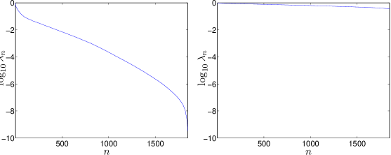
Figure 3: Left: The singular values $\lambda_{n}$ ($n:1,\ldots,1848$) of the operators $K^{(1)}$ and $K^{(4)}$. Right: The singular values $\lambda_{n}$ ($n:1,\ldots,1848$) of the operators $K^{(2)}$ and $K^{(3)}$. The Gaussian random matrix $K^{(2)}$ is much better conditioned than operator $K^{(1)}$.

4.1 A severely ill-conditioned operator

In figure 4, we compare the six algorithms (a)–(e) mentioned in section 2 for the same ill-conditioned operator $K^{(1)}\in\mathbb{R}^{1848\times 8192}$ as in figure 2. We again choose penalty parameters $\lambda_{\mathrm{max}}\geq\lambda\geq\lambda_{\mathrm{max}}/2^{14}$ and show the isochrones corresponding to $t=1,2,\ldots,10$ minutes. Panel (a) is identical to figure 2. All six algorithms do well for large penalties (left-hand sides of the graphs). For smaller values of $\lambda$ ($8<\log_{2}\lambda_{\mathrm{max}}/\lambda$) the isochrones come closer together meaning that convergence progresses very slowly for algorithms (a), (a’), (b) and (c). For algorithm (d), the isochrones are still reasonable uniformly spaced even for smaller values of the penalty parameter. In this case the projected algorithms do better than iterative thresholding, but the $\ell_{1}$-ls algorithm (d) is to be preferred in case of small penalty parameters. The Fista (e) algorithm seems to perform best of all for small parameters $\lambda$.

Figure 4: These pictures contain the approximation isochrones for the algorithms (a)–(e) mentioned in section 2 for $t=1,2\ldots 10$ minutes. The horizontal and vertical axis are identical to the ones used in figure 2. The operator used is $K^{(1)}$. Clearly, for this example, methods (a), (a’), (b) and (c) have a lot of difficulty approaching the minimizer for small values of $\lambda$ (closely spaced isochrones). The $\ell_{1}$-ls method (d) still works well, but it is slower for large penalties. The Fista methods (e) appears to work best for small penalty parameters. The GPSR method works well for relatively large values of $\lambda$. See text for a discussion.

Apart from the shape of the isochrone curves, it is also important to appreciate the top horizontal scales of these plots. The top scale indicate the size of the support of the corresponding minimizer $\bar{x}(\lambda)$. We see that all algorithms have much difficulty in finding minimizers with more than about $100$ nonzero components. In this range of the number of nonzero components in $\bar{x}(\lambda)$, the direct method is faster for $K^{(1)}$.

A skeptic might argue that, in the case of figures 2 and 4, the minimizer $\bar{x}(\lambda)$ might not be unique for small values of $\lambda$, and that this is the reason why the isochrones do not tend to $e=0$ after about 10 minutes ($\approx 4500$ iterations). This is not the case. If one runs the iterative methods for a much longer time, one sees that the error $e$ does go to zero. Such a plot is made in figure 5 for one choice of $\lambda$ ($\lambda\approx\lambda_{\mathrm{max}}/2^{11.115}$).

Figure 5: Main graph: Relative error $\|x^{(n)}-\bar{x}\|/\|\bar{x}\|$ as a function of time for one particular value of $\lambda$. The operator is $K^{(1)}$. Clearly, all algorithms converge to the same limit $\bar{x}$, but some algorithms are very slow. Inset: zoom-in on the first 10 minutes for the iterative thresholding algorithm. It appears to indicate convergence (to a different minimizer), but this is deceptive as the main graph shows. Labels (a)–(e) refer to the algorithms mentioned in section 2 and figure 4.

What we notice here is that, for iterative soft-thresholding, $\|x^{(n+1)}-x^{(n)}\|/\|x^{(n)}\|=\|x^{(n)}-S_{\lambda}[x^{(n)}+K^{T}(y-Kx^{(n)})\|/\|x^{(n)}\|$ is small ($\approx 10^{-5}$ after $4500$ iterations in this example). But this does not mean that the algorithm has almost converged (as might be suggested by figure 5-inset); on the contrary it indicates that the algorithm is progressing only very slowly for this value of $\lambda$! The difference $\|x^{(n+1)}-x^{(n)}\|/\|x^{(n)}\|$ should be of the order $10^{-16}$, for one to be able to conclude convergence, as already announced in formula (7).

4.2 A Gaussian random matrix

In this subsection we choose $K=K^{(2)}$. It is much less ill-conditioned than the matrix in the previous subsection.

In figure 6 we make the same comparison of the six iterative algorithms (a)–(e) for the operator $K^{(2)}$. We choose penalty parameters $\lambda_{\mathrm{max}}\geq\lambda\geq\lambda_{\mathrm{max}}/2^{14}$ and show the isochrones corresponding to $t=6,12,\ldots,60$ seconds. I.e. the time scale is $10$ times smaller than for the ill-conditioned matrix $K^{(1)}$ in the previous section. Again all the algorithms do reasonably well for large penalty parameters, but performance diminishes for smaller values of $\lambda$.

Figure 6: These pictures contain the approximation isochrones for the algorithms (a)–(e) mentioned in section 2 for $t=6,12,\ldots,60$ seconds. The operator used in this comparison is the Gaussian random matrix $K^{(2)}$. This matrix is much better conditioned than the matrix $K^{(1)}$ which was used for figures 4. The main differences are faster convergence and, importantly, more nonzero components are recoverable (the top scales, indicating the size of the support of the minimizer, are much larger than in figures 4).

The iterative soft-thresholding method with $\|K^{(2)}\|\approx\sqrt{2}$ in (a’) does slightly better than iterative soft-thresholding with $\|K^{(2)}\|\approx 1$ in panel (a). The GPSR method (c) does better than the other methods for large values of the penalty (up to $|\mathrm{supp}\,\bar{x}|\approx 500$), but loses out for smaller values. The $\ell_{1}$-ls method (d) does well compared to the other algorithms as long as the penalty parameter is not too large. The FISTA method (e) does best except for the very small value of $\lambda$ (right hand sides of plots) where the projected steepest descent does better in this time scale.

Apart from the different time scales ($1$ minute vs. $10$ minutes) there is another, probably even more important, difference between the behavior of the algorithms for $K^{(1)}$ and $K^{(2)}$. In the latter case the size of the support of the minimizers that are recoverable by the iterative algorithms range from $0$ to about $1800$ (which is about the maximum for $1848$ data). This is much more than in the case of the matrix $K^{(1)}$ in figure 4 where only minimizers with about $120$ nonzero coefficients were recoverable.

4.3 Further examples

Here we compare the various iterative algorithms for the operators $K^{(3)}$ and $K^{(4)}$. The former was constructed such that many elements of its null space are almost parallel to the edges of the $\ell_{1}$ ball, in an effort to make the minimization (1) more challenging. The latter operator has the same singular vectors as the random Gaussian matrix $K^{(2)}$ but the ill-conditioned spectrum of $K^{(1)}$. This will then illustrate how the spectrum of $K$ can influence the algorithms used for solving (1).

Figure 7 shows the isochrone lines for the various algorithms applied to the operator $K^{(3)}$. To make comparison with figure 6 straightforward, the total time span is again $1$ minute subdivided in $6$s intervals. Convergence first progresses faster than in figure 6: the isochrone corresponding to $t=6$s lies lower than in figure 6. For $\lambda<\lambda_{\mathrm{max}}/2^{6}$ it is clear that the various algorithms perform worse for the operator $K^{(3)}$ than for the matrix $K^{(2)}$. As these two operators have identical spectra, this implies that a well-conditioned spectrum alone is no guarantee for good performance of the algorithms.

Figure 7: The six algorithms (a)–(e) are compared for the operator $K^{(3)}$. The time intervals are again $6,12,\ldots,60$s. For $\lambda<\lambda_{\mathrm{max}}/2^{6}$, the algorithms performs worse than in the case of matrix $K^{(2)}$ in figure 6, although $K^{(2)}$ and $K^{(3)}$ have the same singular values.

Figure 7 shows the isochrone plots for the operator $K^{(4)}$ which has identical spectrum as $K^{(1)}$, implying that it is very ill-conditioned. The singular vectors of $K^{(4)}$ are the same as for the random Gaussian matrix $K^{(2)}$. We see that the ill-conditioning of the spectrum influences the performance of the algorithms is a negative way, as compared to the Gaussian operator $K^{(2)}$.

Figure 8: The six algorithms (a)–(e) are compared in case of the operator $K^{(4)}$. The time intervals are $1,2,\ldots,10$m as opposed to $6,\ldots,60$s in figure 6. Clearly, replacing the spectrum of the random Gaussian matrix $K^{(2)}$ by the spectrum of $K^{(1)}$, and leaving the singular vectors unaltered, changes the behavior of the minimization algorithms in a negative way. Convergence is much slower than in figure 6 for all algorithms.

4.4 Warm-start strategies

For the warm-start algorithms (A)–(B), it is not possible to draw isochrones because these methods are not purely iterative. They depend on a preset maximum number of iterates and a preset end value for the penalty parameter $\lambda$ or the $\ell_{1}$ norm $\rho$ of $x$. It is possible, for a fixed total computation time and a fixed value of $\lambda_{\mathrm{stop}}$ or $\rho_{\mathrm{stop}}$, to plot $\|\bar{x}(\lambda_{n})-x^{(n)}\|$ vs. $\lambda_{n}$ or $\|\tilde{x}(\rho_{n})-x^{(n)}\|$ vs. $\rho_{n}$. This gives a condensed picture of the performance of such an algorithm, as it include information on the remaining error for various values of $\lambda$ or $\rho$.

In figure 9, the warm-start methods (A) and (B) are compared in the range $0\leq\|\bar{x}\|_{1}\leq 15$ for the matrix $K^{(1)}$. For each experiment, ten runs were performed, corresponding to total computation times of $1,2,\ldots,10$ minutes. For each run, the parameter $\rho_{\mathrm{max}}$ was chosen to be 15 in algorithm (B). For algorithm (A), $\lambda_{\mathrm{stop}}$ was chosen such that $\|\bar{x}(\lambda_{\mathrm{stop}})\|_{1}=15$ also. From the pictures we see that the algorithms (A)–(B) do not do very well for small values of the penalty parameter $\lambda$. Their big advantage is clear: For the price of a single run, an acceptable approximation of all minimizers $\bar{x}(\lambda)$ with $\lambda_{\mathrm{max}}\geq\lambda\geq\lambda_{\mathrm{stop}}$ is obtained. The algorithm (B) does somewhat better than algorithm (A).

Figure 9: The behavior of two warm-start strategies for the operator $K^{(1)}$. The labels (A)–(B) refer to the list in section 2. In each picture the top line corresponds to a total calculation time of $1$ minute. The bottom line corresponds to $10$ minutes total calculation time (this is about $4800$ iterative soft-thresholding steps or $3000$ projected steepest descent steps). The lines in these plots are not isochrones, as these algorithms are not purely iterative, but depend on a preset stopping radius $\rho_{\mathrm{stop}}$ or stopping penalty $\lambda_{\mathrm{stop}}$. $\rho_{\mathrm{stop}}$ equals $15$ in this case.

In figure 10, the same type of comparison is made for the matrix $K^{(2)}$. In this case, ten runs are performed with a total computation time per run equal to $6,12,\ldots,60$ seconds ($60$s corresponds to about $460$ iterative soft-thresholding steps or $300$ projected steepest descent steps). This is ten times less than in case of the matrix $K^{(1)}$. Both the ‘fixed point continuation method’ (A) and the ‘projected steepest descent’ (B) do acceptably well, even up to very small values for the penalty parameter $\lambda$ (large value of $\rho$).

Figure 10: The behavior of two warm-start strategies for the Gaussian random matrix $K^{(2)}$. In each picture the top line corresponds to a total calculation time of $6$ seconds. The bottom line to $1$ minute. In this case we chose to stop at $\lambda_{\mathrm{stop}}$ equals $\lambda_{\mathrm{max}}/2^{12}$.

All the calculations in this note were done on a 2GHz processor and 2Gb ram memory.

5 Conclusions

The problem of assessing the convergence properties for $\ell_{1}$ penalized least squares functionals was discussed.

We start from the rather obvious observation that convergence speed can only refer to the behavior of $e=\|x^{(n)}-\bar{x}\|/|\bar{x}\|$ as a function of time. Luckily, in the case of functional (1), the exact minimizer $\bar{x}$ (up to computer round-off) can be found in a finite number of steps: even though the variational equations (4) are nonlinear, they can still be solved exactly using the LARS/homotopy method. A direct calculation of the minimizers $\bar{x}(\lambda)$ is thus possible, at least when the number of nonzero coefficients in $\bar{x}$ is not too large (e.g. in the numerical experiments in [7], one has $4096$ degrees of freedom and only about 160 nonzeros.).

We provided a graph that indicates the time complexity of the exact algorithm as a function of $s$, the number of nonzero components in $\bar{x}(\lambda)$. It showed us that computing time rises approximately cubically as a function of $s$ (it is linear at first). Also we gave an example where the size of support of $\bar{x}(\lambda)$ does not decrease monotonically as $\lambda$ decreases. The direct method is certainly practical for $|\,\mathrm{supp}\,\bar{x}(\lambda)|\leq 10^{3}$ or so.

It is impossible to completely characterize the performance of an iterative algorithm in just a single picture. A good qualitative appreciation, however, can be gained from looking at the approximation isochrones introduced in this note. These lines in the $\lambda-e$-plane tell us for which value of the penalty parameter $\lambda$ convergence is adequately fast, and for which values it is inacceptably slow. We look at the region $e\in[0,1]$, because this is probably most interesting for doing real inversions. One could also use a logarithmic scale for $e$, and look at very small values of $e$ approaching computer epsilon. But that is probably not of principle interest to people doing real inverse problems. The main content is thus in the concept of approximation isochrone and in figures 2, 4, 6, 7 and 8 comparing six different algorithms for four operators.

For large penalty parameters, all algorithms mentioned in this note do well for our particular example operators with a small preference for the GPSR method. The biggest difference can be found for small penalty parameters. Algorithms (a), (a’), (b) and (c) risk to be useless in this case. The $\ell_{1}$-ls (d) algorithm seems to be more robust, but it loses out for large penalties. The FISTA method (e) appears to work best for small values of the penalty parameter.

We uncovered two aspects that may influence the convergence speed of the iterative algorithms. Firstly we saw that convergence is slower for ill-conditioned operators than for well-conditioned operators (comparison of $K^{(2)}$ and $K^{(4)}$). Furthermore, the number of nonzero coefficients that a recoverable minimizer has is smaller for an ill-conditioned operator. In particular, the operator $K^{(1)}$ that comes out of a real physical problem, presents a challenge for all algorithms for small values of the penalty parameter. Secondly, the orientation of the null-space with respect to the edges of the $\ell_{1}$ ball also influences the speed of convergence of the iterative algorithms, even if the operator is well-conditioned (comparison of $K^{(2)}$ and $K^{(3)}$).

We also compared two warm-start strategies and showed that their main advantage is to yield a whole set of minimizers (for different penalty parameters) in a single run. We found that the adaptive-steepest descent method (B), proposed in [5] but tested here for the first time, does better than the fixed point continuation method (A).

6 Acknowledgments

Part of this work was done as a post-doctoral research fellow for the F.W.O-Vlaanderen (Belgium) at the Vrije Universiteit Brussel and part was done as ‘Francqui Foundation intercommunity post-doctoral researcher’ at Département de Mathématique, Université Libre de Bruxelles. Discussions with Ingrid Daubechies and Christine De Mol are gratefully acknowledged. The author acknowledges the financial support of the VUB through the GOA-62 grant, of the FWO-Vlaanderen through grant G.0564.09N.

References

- [1] D.L. Donoho. Compressed sensing. Information Theory, IEEE Transactions on, 52(4):1289–1306, 2006.
- [2] I. Daubechies, M. Defrise, and C. De Mol. An iterative thresholding algorithm for linear inverse problems with a sparsity constraint. Communications On Pure And Applied Mathematics, 57(11):1413–1457, November 2004.
- [3] Fadil Santosa and William W. Symes. Linear inversion of band-limited reflection seismograms. SIAM J. Sci. Stat. Comput., 7:1307–1330, 1986.
- [4] R. Tibshirani. Regression shrinkage and selection via the lasso. J. Royal. Statist. Soc B., 58:267–288, 1996.
- [5] I. Daubechies, M. Fornasier, and I. Loris. Accelerated projected gradient method for linear inverse problems with sparsity constraints. Journal of Fourier Analysis and Applications, 2008. Accepted.
- [6] S.-J. Kim, K. Koh, M. Lustig, S. Boyd, and D. Gorinevsky. A method for large-scale -regularized least squares problems with applications in signal processing and statistics. IEEE Journal on Selected Topics in Signal Processing, 2007. Accepted.
- [7] Mario A. T. Figueiredo, Robert D. Nowak, and Stephen J. Wright. Gradient projection for sparse reconstruction: Application to compressed sensing and other inverse problems. To appear in the IEEE Journal of Selected Topics in Signal Processing: Special Issue on Convex Optimization Methods for Signal Processing, 2008.
- [8] Elaine T. Hale, Wotao Yin, and Yin Zhang. A fixed-point continuation method for -regularized minimization with applications to compressed sensing. Technical report, Rice University, 2007.
- [9] Amir Beck and Marc Teboulle. A fast iterative shrinkage-thresholding algorithm for linear inverse problems. SIAM Journal on Imaging Sciences, 2008. To appear.
- [10] Ignace Loris, Guust Nolet, Ingrid Daubechies, and F. A. Dahlen. Tomographic inversion using -norm regularization of wavelet coefficients. Geophysical Journal International, 170(1):359–370, 2007.
- [11] M. R. Osborne, B. Presnell, and B. A. Turlach. A new approach to variable selection in least squares problems. IMA J. Numer. Anal., 20(3):389–403, July 2000.
- [12] Bradley Efron, Trevor Hastie, Iain Johnstone, and Robert Tibshirani. Least angle regression. Ann. Statist., 32(2):407–499, 2004.
- [13] K. Sjöstrand. Matlab implementation of LASSO, LARS, the elastic net and SPCA, jun 2005. Version 2.0.
- [14] David Donoho, Victoria Stodden, and Yaakov Tsaig. About SparseLab, March 2007.
- [15] Ignace Loris. L1Packv2: A Mathematica package for minimizing an -penalized functional. Computer Physics Communications 179: 895–902, 2008.
- [16] Patrick L. Combettes and Valerie R. Wajs. Signal recovery by proximal forward-backward splitting. Multiscale Model. Simul., 4(4):1168–1200, January 2005.
- [17] P.L. Combettes. Convex set theoretic image recovery by extrapolated iterations of parallel subgradient projections. Image Processing, IEEE Transactions on, 6(4):493–506, 1997.