Noise-induced bifurcations, Multiscaling and On-Off intermittency

Abstract

We present recent results on noise-induced transitions in a nonlinear oscillator with randomly modulated frequency. The presence of stochastic perturbations drastically alters the dynamical behaviour of the oscillator : noise can wash out a global attractor but can also have a constructive role by stabilizing an unstable fixed point. The random oscillator displays a rich phenomenology but remains elementary enough to allow for exact calculations : this system is thus a useful paradigm for the study of noise-induced bifurcations and is an ideal testing ground for various mathematical techniques. We show that the phase is determined by the sign of the Lyapunov exponent (which can be calculated non-perturbatively for white noise), and we derive the full phase diagram of the system. We also investigate the effect of time-correlations of the noise on the phase diagram and show that a smooth random perturbation is less efficient than white noise. We study the critical behaviour near the transition and explain why noise-induced transitions often exhibit intermittency and multiscaling : these effects do not depend on the amplitude of the noise but rather on its power spectrum. By increasing or filtering out the low frequencies of the noise, intermittency and multiscaling can be enhanced or eliminated.

I Introduction

Most patterns observed in nature are created by instabilities that occur in an uncontrolled noisy environment : convection in the atmospheric layers and in the mantle are subject to inhomogeneous and fluctuating heat flux; sand dunes are formed under winds with fluctuating directions and strengths. These fluctuations usually affect the control parameters driving the instabilities, such as the Rayleigh number which is proportional to the imposed temperature gradient in natural convection. These fluctuations act multiplicatively on the unstable modes. In the same spirit, the evolution of global quantities, averaged under small turbulent scales, can be represented by a nonlinear equation with fluctuating global transport coefficients that reflect the complexity at small scales. For instance, it has been shown that the temporal evolution of the total heat flux in rotating convection can be described by a non–linear equation with a multiplicative noise Neufeld . The dynamo instability that describes the growth of the magnetic field of the earth and the stars because of the motion of conducting fluids in their cores, is usually analyzed in similar terms : the magnetic field is expected to grow at large scale, forced by a turbulent flow. Here again, the parameters controlling the growth rate of the field are fluctuating Sweet .

Since the theoretical predictions of Stratonovich Strato , and the experimental works of Kawaboto, Kabashima and Tsuchiya Kawakubo , it is well known that the phase diagram of a system can be drastically modified by the presence of noise graham ; lefever . Because of stochastic fluctuations of the control parameter, the critical value of the threshold may change and noise can delay or favor a phase transition vankampen ; gardiner ; risken ; anishchenko . When a physical system subject to noise undergoes bifurcations into states that have no deterministic counterparts, the stochastic phases generated by randomness have specific characteristics (such as their scaling behavior and the associated critical exponents) allowing to define new universality classes munoz1 .

A straightforward approach to study the effect of noise on a bifurcation diagram would consist in analyzing the nonlinear Langevin equation that governs the system. However, the interplay between noise and nonlinearity results in subtle effects that make nonlinear stochastic differential equations hard to handle vankampen ; wax ; arnold . One of the simplest systems that can be used as a paradigm for the study of noise-induced phase transitions is the random frequency oscillator (for a recent and detailed monograph devoted to this subject see gitterman ). A deterministic oscillator with damping evolves towards the equilibrium state of minimal energy that represents the unique asymptotic state of the system. However, if the frequency of the oscillator is a time-dependent variable, the behavior may change : due to continuous energy injection into the system through the frequency variations, the system may sustain non-zero oscillations even in the long time limit if the amplitude of the noise is large enough.

In this work, we present recent results on noise-induced transitions in a nonlinear oscillator with randomly modulated frequency. The ouline of this article is as follows.

In section II, we show that an explicit calculation of the Lyapunov exponent allows to determine exactly the phase diagram of the noisy Duffing oscillator philkir1 ; philkir2 . In the case of a single-well oscillator, a large enough noise destabilizes the origin (which is a fixed point for the deterministic dynamics). The double-well oscillator presents a richer structure : the unstable fixed point becomes a global attractor of the stochastic dynamics when the amplitude of the noise lies in a well-defined interval : this is a typical example of a reentrant transition (which was observed earlier in the more elaborate setting of spatially extended systems vdbtorral ). These properties are only qualitatively modified when the noise has temporal correlations.

In section III, we discuss the scaling exponents associated with the order parameter in the vicinity of the transition. For a deterministic transition, it is well-known that the different types of bifurcations can be classified by some characteristic exponents. We show, in the stochastic case, that these exponents can be modified by the noise : the dynamical variable has a non-trivial scaling behaviour and its time series exhibits on-off intermittency. Following seb1 ; seb2 , we explain that multiscaling and intermittency are intimately linked with each other and that their existence is due to the presence of low frequency components in the noise spectrum. By using a random process with a spectral structure richer than that of white or Ornstein-Uhlenbeck noise, we show that the deterministic exponents can be recovered by a suitable low-band flitering of the noise. This fact implies that the concept of critical exponents can be ambiguous for noise-induced bifurcations and is certainly not as useful as it is for deterministic phase transitions.

Section IV presents a discussion on perturbative perturbative expansion of the nonlinear Langevin equation. Whereas most studies rely on Fokker-Planck type evolution equations for the Probability Distribution Function (PDF) in which the noise is integrated out by mapping a stochastic ordinary differential equation into a deterministic partial differential equation in the phase space of the system, it is also possible to perform a direct perturbative expansion of the nonlinear Langevin equation by using the classical Poincaré-Lindstedt method luecke1 ; luecke2 . This technique has the advantage as compared to the more traditional approaches of being applicable to a noise with an arbitrary spectrum (whereas Fokker-Planck equations are only valid for white-noise). However, due to the presence of low-frequencies in the noise spectrum, the perturbative expansion breaks down and diverges. This divergence is at the origin of the multiscaling behaviour and of the anomalous scaling exponents. The last section is devoted to concluding remarks.

II Stochastic Bifurcations of a random parametric oscillator

In this section, we present the phase diagram of a nonlinear oscillator with a randomly modulated frequency. The case when the frequency is a periodic function of time is a classical problem known as the Mathieu oscillator drazin ; nayfeh ; kevorkian . The phase diagram of the (damped) Mathieu oscillator is obtained by calculating the Floquet exponents (defined as the characteristic growth rates of the amplitude of the system). This phase diagram presents an alternance of stable regions in which the system evolves towards its equilibrium state and of unstable regions in which, because of parametric resonance, the amplitude of the oscillations grows without bound. A nonlinear term is needed to saturate these oscillations. When the frequency of the pendulum is a random process, the role of the Floquet exponents is taken over by the Lyapunov exponents. The system undergoes a bifurcation when the largest Lyapunov exponent, defined as the growth rate of the logarithm of the energy, changes its sign. Thus, the Lyapunov exponent vanishes on the critical surface that separates the phases in the parameter space. This criterion involving the sign of the Lyapunov exponent resolves the ambiguities that were found in studies of the stability of higher moments bourret ; bourretFrisch ; lindenberg3 and has a firm mathematical basis arnold . In recent works philkir1 ; philkir2 , we have obtained the exact phase diagram of the random oscillator when the frequency is a Gaussian white noise. In the last part of this section, we discuss the effect of non-vanishing time-correlation in the noise kirPeyneau .

II.1 Instability induced by noise: the single-well oscillator

The equation for the amplitude $x$ of a random Duffing oscillator with a fluctuating frequency is

$$\ddot{x}+\gamma\dot{x}+(\omega^{2}+\xi(t))\,x+\lambda x^{3}=0\,,$$ (1)

where $\gamma$ is the (positive) friction coefficient, $\omega$ the mean frequency and$\lambda$ the coefficient of the cubic non-linear term. The random fluctuations of the frequency are represented by a Gaussian white noise $\xi(t)$ of zero mean-value and of amplitude ${\mathcal{D}}$

$$\langle\xi(t)\rangle = 0\,,$$

$$\langle\xi(t)\xi(t^{\prime})\rangle = {\mathcal{D}}\,\delta(t-t^{\prime})\,.$$ (2)

In this work, all stochastic differential equations are interpreted according to Stratonovich calculus. By rewriting time and amplitude in dimensionless units, $t:=\omega t$ and $x:=\lambda^{1/2}\omega^{-1}x,$ Eq. (1) becomes

$$\frac{\mathrm{d}^{2}x}{\mathrm{d}t^{2}}+\alpha\,\frac{\mathrm{d}x}{\mathrm{d}t}+x+x^{3}=x\,\Xi(t),$$ (3)

where $\Xi(t)$ is a delta-correlated Gaussian variable with vanishing mean value and with correlations given by

$$\langle\Xi(t)\Xi(t^{\prime})\rangle = \Delta\,\delta(t-t^{\prime})\,.$$ (4)

The parameters

$$\alpha=\gamma/\omega\,\,\,\,\,\hbox{ and }\,\,\,\,\,\Delta={\mathcal{D}}/\omega^{3}$$ (5)

correspond to dimensionless dissipation rate and to noise strength, respectively.

The equation (1) has the origin of the phase space, $\dot{x}=x=0$, as a fixed point. When the system is deterministic, i.e., when ${\mathcal{D}}=0$, the origin is a global attractor for any $\gamma>0$ : for any initial condition we know that $x(t)\to 0$ and $\dot{x}(t)\to 0$ when $t\to\infty$.

However, in presence of noise, the asymptotic behaviour of the system becomes more complex. In Fig. 1, we present, for three values of the parameters, a trajectory in the phase plane $(x,v=\dot{x})$ characteristic of the oscillator’s behaviour, using the numerical one step collocation method advocated in mannella . Initial conditions are chosen far from the origin, with an amplitude of order $1$. Noisy oscillations are observed for small values of the damping parameter $\alpha$ [See Fig. 1.a]. For larger values of $\alpha$ the origin becomes a global attractor for the dynamics [See Fig. 1.b]. Increasing the noise amplitude $\Delta$ at constant $\alpha$ makes the origin unstable again [See Fig. 1.c].

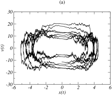
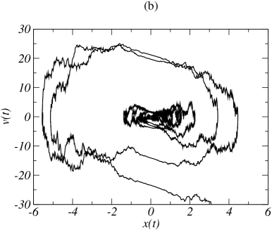
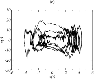
Figure 1: Phase plane plots of a typical trajectory of the noisy nonlinear oscillator. Eq. (3) is integrated numerically with a time step $\delta t=5\ 10^{-4}$. (a) $\alpha=0.5$, $\Delta=20$, $t\leq 100$; (b) $\alpha=2.0$, $\Delta=20$, $t\leq 100$; (c) $\alpha=2.0$, $\Delta=60$, $t\leq 100$. Early-time relaxation towards noisy oscillations has been omitted for clarity in cases (a) and (c). The trajectory spirals down towards the origin in case (b).

In other words, for the stochastic oscillator, the following property is true : For a given $\gamma$ there is a critical noise amplitude $\mathcal{D}_{c}(\gamma)$ such that

$$\mathcal{D}<\mathcal{D}_{c}(\gamma) \,\,\,\,\,\,\dot{x},x\to 0\,\,\,\hbox{ when }t\to\infty$$

$$\mathcal{D}>\mathcal{D}_{c}(\gamma) \,\,\,\,\,\,\dot{x},x\to\hbox{ Oscillating Stationary State}$$

The main problem is to calculate the value of $\mathcal{D}_{c}$ as a function of $\gamma$ and the other parameters of the problem.

For random dynamical systems, it was recognized early on that various ‘naive’ stability criteria bourret ; bourretFrisch , obtained by linearizing the dynamical equation around the origin, lead to ambiguous results. This feature is in contrast with the deterministic case for which the bifurcation threshold is obtained without ambiguity by studying the eigenstates of the linearized equations manneville . For the random oscillator, trying to determine the critical noise amplitude by studying the stability of the moments of the amplitude of the linearized equations leads to inconsistent results. More precisely, consider the random harmonic oscillator, obtained by linearizing equation (1) near the origin :

$$\ddot{x}+\gamma\dot{x}+(\omega^{2}+\xi(t))\,x=0\,.$$ (6)

The second moment $\langle x^{2}\rangle$ of the amplitude of the linearized equation converges to 0 in the long time limit if

$$\frac{\mathcal{D}}{\omega^{3}}<2\frac{\gamma}{\omega}\,.$$

The fourth moment $\langle x^{4}\rangle$ converges to 0 if

$$\frac{\mathcal{D}}{\omega^{3}}<\frac{2\gamma}{3\omega}\,\frac{3\gamma^{2}+4\omega^{2}}{3\gamma^{2}+2\omega^{2}}\,.$$

More generally, the moment $\langle x^{2p}\rangle$ is stable if

$$\frac{\mathcal{D}}{\omega^{3}}<\frac{2}{2p-1}\frac{\gamma}{\omega}{\mathcal{F}}_{p}\left(\frac{\gamma}{\omega}\right)\,.$$

In fact, it was conjectured in bourretFrisch and proved in lindenberg3 that, in a linear oscillator with arbitrarily small parametric noise, all moments beyond a certain order grow exponentially in the long time limit. In figure 2, we plot the stability diagram for the moments of order 2,4 and 6. We observe that the stability range becomes narrower when the order of the moment becomes higher. This means that any criterion based on finite mean displacement, momentum, or energy of the linearized dynamical equation is not adequate to show the stability of the initial problem and the bifurcation threshold of a nonlinear random dynamical system cannot be determined simply from the moments of the linearized system. In practice, the phase diagram of the non-linear random oscillator was usually determined in a perturbative manner by using weak noise expansions luecke1 ; luecke2 ; landa ; drolet ; landaMc .

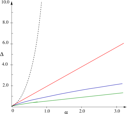
Figure 2: Stability diagram of the moments of the single-well oscillator. The full curves from top to bottom represent the stability lines of $\langle x^{2}\rangle$, $\langle x^{4}\rangle$ and $\langle x^{6}\rangle$. The dashed curve is the line on which the Lyapunov exponent vanishes.

The reason for this failure is that in the linearized problem the statistics of the variable $x$ is dominated by very large and very rare events that induce the divergence of moments of high order. These rare events are suppressed by the nonlinearity and the bifurcation threshold becomes well defined. We face the following paradoxes : (i) the stability region of the origin $\dot{x}=x=0$ for the non-linear equation has a well defined threshold for any value of the noise amplitude : below this threshold the origin is a global attractor of the dynamics. On the contrary the linearized equation does not have a clear-cut bifurcation threshold. (ii) Close to the origin the non-linear term is irrelevant but the nonlinearity has to be taken into account to suppress the rare events that spoil the statistical behaviour of the system.

The problem is to find the correct stability criterion for the non-linear equation that can be formulated as in the deterministic case on the linear equation and that would allow explicit calculations.

Such a criterion does exist and is based on the Lyapunov exponent that measures the growth rate of the random harmonic oscillator’s energy

$$\Lambda=\lim_{t\to\infty}\frac{1}{2t}\langle\log E\rangle\,\,\,\,\hbox{ with }\,\,\,E=\frac{\dot{x}^{2}}{2}+\omega^{2}\frac{x^{2}}{2}\,,$$ (7)

where $x(t)$ is a solution of equation (6). It has been shown (see philkir1 and references therein) that when the Lyapunov exponent is negative the Fokker-Planck equation has a unique stationary solution which is the Dirac delta function at the origin of the phase space. This means that the origin is a stable global absorbing state. However, when the Lyapunov exponent is positive and extended, stationary probability distribution function exists and describes an oscillatory asymptotic state of the nonlinear random oscillator. These features are reminiscent of Anderson localization and there exists indeed a mapping between the random oscillator and a 1d localization model tessieri ; jmluck .

The equation of the transition line that determines the stability of the origin for the nonlinear oscillator with a random phase is therefore given by

$$\boxed{\,\,\,\,\,\,\,\,\Lambda(\gamma,\omega,\mathcal{D})=0\,.\,\,\,\,\,\,\,\,}$$ (8)

The following exact closed formula for the Lyapunov exponent of the system can be derived when the random frequency modulation is a Gaussian white noise hansel ; imkeller ; philkir1  :

$$\Lambda = \frac{\gamma}{2}\left(\frac{\int_{0}^{\infty}\sqrt{u}\,\,\rm{e}^{-\psi(u)}\rm{d}u}{\int_{0}^{\infty}\frac{\rm{d}u}{\sqrt{u}}\,\,\rm{e}^{-\psi(u)}}-1\right)\,$$ (9)

$$\hbox{ with }\psi(u) = \frac{2\gamma^{3}}{\mathcal{D}}\left\{\left(\frac{\omega^{2}}{\gamma^{2}}-\frac{1}{4}\right)u+\frac{u^{3}}{12}\right\}\,.$$ (10)

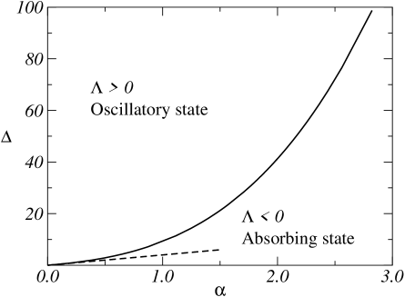
Figure 3: Phase diagram of the single-well oscillator with multiplicative noise. The critical curve separates an absorbing and an oscillatory phase in the $(\alpha,\Delta)$ plane. The dashed line represents the small noise approximation (see text).

Inserting this formula in the stability criterion (8) and using dimensionless variables we obtain the equation of the transition line in the ($\alpha$, $\Delta$) plane. For a given value of $\Delta$, the critical value of the damping $\alpha=\alpha_{c}(\Delta)$ for which the Lyapunov exponent vanishes is given by

$$\alpha_{c}={\displaystyle{\frac{\int_{0}^{+\infty}\mathrm{d}u\;{\sqrt{u}}\;\exp\left\{-\frac{2}{\Delta}\left((1-\frac{\alpha_{c}^{2}}{4})u+\frac{u^{3}}{12}\right)\right\}}{\int_{0}^{+\infty}\frac{\mathrm{d}u}{\sqrt{u}}\exp\left\{-\frac{2}{\Delta}\left((1-\frac{\alpha_{c}^{2}}{4})u+\frac{u^{3}}{12}\right)\right\}}}.}$$ (11)

The critical curve $\alpha=\alpha_{c}(\Delta)$ is represented in Fig. 3. It separates two regions in parameter space: for $\alpha<\alpha_{c}$ (resp. $\alpha>\alpha_{c}$) the Lyapunov exponent is positive (resp. negative), the stationary PDF is an extended function (resp. a delta distribution) of the energy and the origin is unstable (resp. stable). For small values of the noise amplitude, it can be shown that the exact formula (11) reduces at first order to the linear relation $\alpha_{c}=\frac{\Delta}{4},$ in agreement with previous perturbative calculations. For large values of the noise, we obtain $\alpha_{c}\simeq 0.656\Delta^{1/3}\,.$ We emphasize that the phase diagram drawn in Fig. 3 is exact for all values of the noise amplitude $\Delta$ and the damping parameter $\alpha$.

II.2 Stabilisation by noise: the double-well oscillator

In a classical calculation, Kapitza (1951) showed that the unstable upright position of an inverted pendulum is stabilised if its suspension axis undergoes sinusoidal vibrations of high enough frequency. Analytical derivations of the stability limit are based on perturbative approaches, i.e., in the limit of small forcing amplitudes landau ; nayfeh ; barma .

When the sinusoidal vibrations of the suspension axis are replaced by a white noise, an exact, non-perturbative, stability analysis can be performed philkir2 . In particular, for the stochastic inverted pendulum, we have shown that the unstable fixed point can be stabilized by noise and have discovered the existence of a noise-induced reentrant transition.

The general equation for the Duffing oscillator subject to multiplicative noise is given by :

$$\ddot{x}+\gamma\dot{x}-(\mu+\xi(t))\,x+x^{3}=0\,.$$ (12)

When $\mu<0$, the non-linear potential has a single-well. This case is the same as the one discussed in the previous section : the origin is deterministically a global attractor that can become unstable in presence of noise. When $\mu>0$, the oscillator is subject to a double-well potential and the origin is deterministically unstable.

Figure 4: The double-well oscillator with parametric noise

In presence of noise, the correct criterion for stability analysis is again based on the sign of the Lyapunov exponent. In order to take into account both possible signs of $\mu$, it is useful to define the following set of dimensionless parameters :

$$\alpha=\frac{\mu}{\gamma^{2}}\,\,\,\,\hbox{ and }\Delta=\frac{{\mathcal{D}}}{\gamma^{3}}\,.$$ (13)

An exact calculation of the Lyapunov exponent philkir2 then allows to draw the phase diagram represented in figure (5).

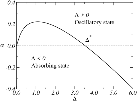
Figure 5: Phase diagram of the double-well oscillator subject to multiplicative Gaussian white noise. The solid line is the locus where $\Lambda(\alpha,\Delta)=0$. The bifurcation line $\alpha=0$ of the noiseless dynamical system is drawn for comparison (dotted line). For $\Delta\leq\Delta^{*}\simeq 3.55$ (resp. $\Delta\geq\Delta^{*}$), the origin is stabilised (resp. destabilised) by the stochastic forcing in the range $0\leq\alpha\leq\alpha_{c}(\Delta)$ (resp. $\alpha_{c}(\Delta)\leq\alpha\leq 0$).

We observe that when $\alpha<0.21\ldots$, there exits a range of noise amplitudes for which the origin is stabilized by noise : for $\Delta$ such that $\Delta_{1}(\alpha)<\Delta<\Delta_{2}(\alpha)$ the origin becomes an attractive fixed point of the stochastic dynamics. The values $\Delta_{1}(\alpha)$ and $\Delta_{2}(\alpha)$ that determine the stability interval are known analyticaly. We emphasize that these functions can not be calculated perturbatively by using a small noise expansion when $\alpha$ is finite. For $\alpha>0.21\ldots$, the stability interval does not exist anymore : the origin is always unstable and the non-equilibrium stationary state exhibits an oscillatory behaviour.

Figure 6: Stability range for the double-well oscillator : when $\alpha<0.21$, the unstable equilibrium point is stabilized by noise for noise amplitudes between $\Delta_{1}$ and $\Delta_{2}$.

II.3 The effect of colored noise

We now discuss the phase diagram of an oscillator whose frequency is a random process with finite time memory. More precisely, we consider the case of an Ornstein-Uhlenbeck noise $x(t)$ of correlation time $\tau$ :

$$\langle\xi(t)\xi(t^{\prime})\rangle = \frac{{\mathcal{D}}_{1}}{2\tau}\exp\left(-|t-t^{\prime}|/\tau\right)\,\,.$$ (14)

When $\tau\to 0$, the process $\xi(t)$ becomes identical to the white noise. The Lyapunov exponent of the system $\Lambda(\omega,\gamma,{\mathcal{D}},\tau)$ becomes now a function of $\tau$ also.

From a physical point of view, the influence of a finite correlation time on the shape of the critical curve is an interesting open question: due to the finite correlation time of the noise, the random oscillator is a non-Markovian random process and there exists no closed Fokker-Planck equation that describes the dynamics of the Probability Distribution Function (P.D.F.) in the phase space. This non-Markovian feature hinders an exact solution in contrast with the white noise case where a closed formula for the Lyapunov exponent was found. For the single-well stochastic oscillator, we have calculated kirPeyneau this Lyapunov exponent by using different approximations and have derived the phase diagram. The main role of the correlation time of the noise, as can be seen in Figure 7, is to enhance the stability region. When $\tau$ grows, amplitude of the noise required to destabilize the origin becomes bigger. This effect can be seen quantitavely in the following exact asymptotic expansions (see also crauel ) :

$$\hbox{ For small values of the noise amplitude~{}:}\,\,\,\alpha_{c} \simeq \frac{\Delta}{4(1+4\omega^{2}\tau^{2})}\,,$$ (15)

$$\hbox{ For large values of the noise amplitude~{}:}\,\,\,\alpha_{c} \simeq C\Big{(}\frac{\Delta}{\omega\tau}\Big{)}^{1/4}\,,$$ (16)

where the constant $C$ is of order 1. Comparing with the white noise result we observe that the behaviour of the critical curve for large noise is modified in presence of time correlations; the asymprtotic exponent is 1/3 for white noise and 1/4 for colored noise even if the correlation time $\tau$ is small. The presence of a non-vanishing correlation time thus modifies the scaling characteristics of the system. This change of scaling at large noise is related to the differentiability properties of the random potential as shown in delyon  : the white noise is continuous but nowhere differentiable whereas the Ornstein-Uhlenbeck process has a first derivative but no second derivative.

Figure 7: Critical curves obtained by numerical simulations of the single-well random oscillator subject to multiplicative Ornstein-Uhlenbeck noise. The curves with black dots ($\bullet$) and with squares ($\Box$) correspond to $\tau=1$ and $\tau=2$, respectively. The full black line is the analytical result for the white noise case.

For the double-well oscillator subject to Ornstein-Uhlenbeck noise, the results of numerical computations of the phase diagram are shown in figure 8. Here also we observe that the noise-inducedstabilization of the deterministically unstable fixed point becomes less efficient in presence of time correlations. In the weak noise limit, this curve agrees with the prediction of luecke1 :$\alpha_{c}(\Delta)\sim\Delta/(2(1+\tau))$. For a noise amplitude of order 1, the bifurcation line is qualitatively similar to that obtained with white noise. However, depending on the value of $\Delta$, the value of the bifurcation point $\alpha_{c}(\Delta)$ is not necessarily a monotonic function of $\tau$. A precise understanding of this non-monotonous behaviour is lacking and the analytical theory of the stability of the double-well oscillator with time-correlated noise still remains to be done. Although the obtention of exact results for the Ornstein-Uhlenbeck noise seems unlikely, various recent works vandenbroeck indicate that the Poisson process provides a useful model for the study of time correlation effects in stochastic systems. The advantage of the Poisson process is that it is amenable to exact analytic calculations.

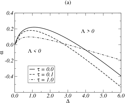
Figure 8: Phase diagram of the double-well oscillator subject to Ornstein-Uhlenbeck noise with correlation time $\tau$. The bifurcation lines for $\tau=0.1$ and $1.0$ are obtained from numerical calculations of the Lyapunov exponent. For comparison, we draw the (analytic) white noise line. In this figure the dimensionless parameters are given by $\alpha=\frac{\omega^{2}}{\gamma^{2}}$ and $\Delta=\frac{{\mathcal{D}}}{\gamma^{3}}\,.$

We conclude this section by emphasizing that the results obtained here for the oscillator with multiplicative noise could be used for other stochastic systems. For example, it has been shown by Schimansky-Geier et al. schimansky that the random Duffing oscillator with additive noise undergoes a phase transition that does not manifest itself in the stationary P.D.F. (which is simply given by the Gibbs-Boltzmann formula). This subtle phase transition, which affects the properties of the random attractor of motion in phase space, can be formulated mathematically as a bifurcation in an associated linear oscillator subject to a multiplicative noise with a a finite correlation time. If we approximate this noise by an effective Ornstein-Uhlenbeck process, the system becomes identical to the one studied here.

III Scaling behaviour near the bifurcation threshold

For deterministic Hopf bifurcation, the amplitude of the order parameter $x$ exhibits a normal scaling behaviour in the vicinity of the transition line; if $\epsilon$ denotes the distance from threshold of the control parameter, we have in the deterministic case :

$$\langle x^{2n}\rangle\sim\epsilon^{n}\,.$$ (17)

We now consider the case of the stochastic oscillator. In figure 9, we plot the behaviour of the amplitude moments in the vicinity of the reentrant transition in a double-well oscillator. The damping rate $\alpha$ is fixed at a given value and the noise strength $\Delta$ is chosen such that $0<\Delta-\Delta_{c}(\alpha)\ll 1$, where $\Delta_{c}(\alpha)$ is the critical value. In this case, the parameters of the system are tuned just above the bifurcation threshold and the Lyapunov exponent is slightly positive: $0<\Lambda\ll 1$. We observe that even-order moments of the amplitude scale linearly with the distance to threshold in the vicinity of the bifurcation line (note that odd-order moments are equal to zero by symmetry) :

$$\boxed{\,\,\,\,\,\,\,\,\langle x^{2n}\rangle\sim\epsilon\,.\,\,\,\,\,\,\,\,}$$ (18)

A similar scaling behaviour is obtained by simulating the single-well oscillator or by replacing white noise by an Ornstein-Uhlenbeck process. Such a behaviour was also observed in random maps pikovsky and in stochastic fields munoz2 . Such a strong multiscaling seems to be a typical feature of stochastic bifurcations and has been noticed a long ago graham in first order stochastic differential equations. The fact that the stochastic oscillator exhibits a similar behaviour can be understood ‘physically’ by noticing that the second order time derivative becomes irrelevant in the long-time limit. The mathematical explanation for this behaviour is also elementary philkir1  : near the bifurcation threshold, when the Lyapunov exponent $\Lambda\to 0$, the stationary Probability Distribution Function $P_{{\rm stat}}$ exhibits a power law divergence at the origin $(\dot{x}=x=0)$, and the region near the origin dominates the statistics : it can be shown that near $E=0$, the stationary energy distribution scales as $P_{{\rm stat}}(E)\sim E^{c\Lambda-1}$ where $c$ is a positive constant. From this formula, one readily deduces that all moments of the energy (and therefore all moments of the amplitude of the oscillator) are of the order $\Lambda$ which itself grows linearly with $\epsilon$, the distance from threshold.

Another remarkable feature of the order parameter near threshold is that the time series $t\mapsto x(t)$ exhibits on-off intermittency. Again this intermittent behaviour, first discovered in coupled dynamical systems yamada and in a system of reaction-diffusion equations pikovskyonoff , is believed to be generic (see e.g., spiegel ) when an unstable system is coupled to a system that evolves in an unpredictable manner (multiplicative noise).

Multiscaling and intermittency lead however to the following very puzzling problems :

Problem 1 : The multiscaling behaviour given in equation (18) is very clearly seen in computer experiments but does not seem to be observed in ‘real’ experiments. Similarly, It is surprising that, despite the genericity of the on-off intermittency mechanism (which is well established mathematically) this effect has scarcely been reported in experiments. One might expect that any careful experimental investigation of an instability should reveal on-off intermittency when the system is close to the onset of instability, and is hence sensitive to unavoidable experimental noise in the control parameters.

Problem 2 : In well known works luecke1 ; luecke2 , it was predicted, using perturbation theory, that the scaling of the stochastic bifurcation should be the same as that of the deterministic Hopf bifurcation, equation (17). This problem is analyzed in section IV.

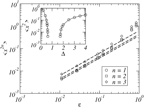
Figure 9: Behaviour of the moments near the reentrant bifurcation threshold. The noisy double-well oscillator subject to parametric white noise is simulated with a fixed parameter $\alpha=0.2$. The critical value of the noise amplitude corresponding to the reentrant transition is found to be $\Delta_{c}\simeq 0.627$ : for a noise amplitude $\Delta$ belonging to the interval (0.627–1.70) the origin is stabilized by the noise. Even-order moments $\langle x^{2}\rangle$, $\langle x^{4}\rangle$ and $\langle x^{6}\rangle$ are plotted versus the distance to threshold $\epsilon=(\Delta_{c}-\Delta)/\Delta_{c}$ (symbols). Dashed lines respecting a linear behaviour $\langle x^{2n}\rangle\propto\epsilon$ are drawn to guide the eye. Inset: the mean square position (measured in the stationary regime) is non-zero for $\Delta<0.627$ and $\Delta>1.70$, i.e., the stationary state is extended.

Problem 1 is solved in seb1 ; seb2 . In these works, it is shown that although the noise strength controls the transition between the absorbing and the oscillatory states, the amplitude of the noise is not the only relevant parameter responsible for multiscaling and intermittency. Rather, these effects are due to the zero-frequency mode of the noise; in other words these effects depend on the Power Spectrum Density (PSD) of the noise and not on its overall amplitude. In order to identify which part of the PSD of the random forcing really affects the dynamics, one needs a random perturbation with a spectral density more complex than that of white noise or of Ornstein-Uhlenbeck noise. A useful type of noise schimanskyharmonic is the harmonic noise $\zeta(t)$ whose autocorrelation function is given by

$$\langle\zeta(t)\,\zeta(t+\tau)\rangle_{s}=A\exp(-2\pi\eta|\tau|)\left(\cos(2\pi\Omega\tau)+\frac{\eta}{\Omega}\sin(2\pi\Omega|\tau|)\right)\,,\,\,\,\,\,\,$$ (19)

where $A$ is the noise amplitude; the corresponding PSD is

$$C(\nu)=\frac{A\eta(\Omega^{2}+\eta^{2})}{\pi[(\Omega^{2}+\eta^{2}-\nu^{2})^{2}+2\nu^{2}\eta^{2}]}\,.$$ (20)

The value of the PDS at zero frequency is therefore given by

$$S=A\eta/\left[\pi(\eta^{2}+\Omega^{2})\right]\,.$$ (21)

For harmonic noise, the amplitude $A$ and the zero frequency amplitude $S$ can be tuned independently.

In figure 10, we plot the time series of a Duffing oscillator with a random frequency perturbation given by a harmonic noise $\zeta(t)$. We observe that the zero frequency amplitude $S$ is the pertinent parameter controlling the intermittent regime : on-off intermittency disappears when the value of $S$ is lowered. For the simple first-order model,

$$\dot{x}=(a+\zeta(t))x-x^{3}\,,$$ (22)

it is possible to determine analytically the transition line between intermittent behaviour and non-intermittent behaviour in the $(S,a)$ plane, using the cumulant expansion introduced by Van Kampen vankampen . Intermittency occurs when

$$0<\frac{a}{S}<1\,.$$ (23)

This criterion is checked numerically in figure 11.

Finally, it is possible to prove that multiscaling is a consequence of the intermittent behaviour of the order parameter $x(t)$ seb2 . Therefore as the zero frequency noise amplitude is reduced, both on-off intermittency and multiscaling are suppressed and normal scaling  (17) is recovered.

This analysis solves Problem 1 by explaining why many experimental investigations on the effect of a multiplicative noise on an instability do not display on-off intermittency. If the noise is high-pass filtered, as often required for experimental reasons, then the regime of intermittent behavior disappears. This is the case for instance in Francois2 : a ferrofluidic layer undergoes the Rosensweig instability and peaks appear at the surface. The layer is then subject to a multiplicative noise through random vertical shaking. Close to the deterministic onset, the unstable mode submitted to a colored noise does not display intermittency. Another experimental obstacle to observe intermittency is the presence of additive noise that destroys the symmetry of the system.

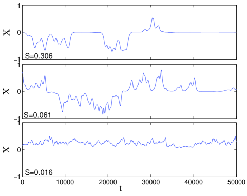
Figure 10: Temporal traces of the amplitude of a Duffing oscillator subject to harmonic noise of constant amplitude $A=0.05$. As the value $S$ of the zero frequency amplitude of the noise is decreased from top to bottom, intermittent behaviour is suppressed.

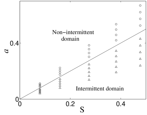
Figure 11: Intermittency phase diagram for the solution of (22) with harmonic noise. ($\triangle$) : intermittent behavior, ($\circ$) : non-intermittent behavior. The full line is the transition curve predicted by (23).

IV Remarks on the perturbative analysis of a noisy Hopf bifurcation

Problem 2 questions the relevance of perturbative expansions for studying noise induced bifurcations. Consider, for example, the parametrically driven damped anharmonic oscillator that naturally appears in the study of many instabilities fauve . Such a system is described by the following equation :

$$m\ddot{x}+m\gamma\dot{x}=\left(\epsilon+\Delta\xi(t)\right)x-x^{3}\,,$$ (24)

where $\epsilon$ is the control parameter and the modulation $\xi(t)$ is of arbitrary dynamics and statistics: it can be a periodic function or a random noise. For small driving amplitudes $\Delta$, Lücke and Schank luecke1 have performed a Poincaré-Lindstedt expansion called the Poincaré-Lindstedt expansion drazin ; kevorkian ; kleinert (see khrustalev for applications to field-theory). They have obtained an expression for the threshold $\epsilon_{c}(\Delta)$ (at first order in $\Delta$). Their result has been verified both numerically and experimentally and is also in agreement with the exact result obtained for the Gaussian white noise (in this case a closed formula is available for $\epsilon_{c}(\Delta)$ for arbitrary values of $\Delta$). Another result obtained in luecke1 ; luecke2 is the scaling of the moments near the threshold,

$$\langle x^{2n}\rangle=s_{n}\left(\epsilon-\epsilon_{c}(\Delta)\right)^{n}+{\mathcal{O}}\left((\epsilon-\epsilon_{c})^{n+1}\right)\,,$$ (25)

where the constant $s_{n}$ depends on $\xi(t)$ and on $\Delta$. The moments have a normal scaling behaviour : $\langle x^{2n}\rangle$ scales as $\langle x^{2}\rangle^{n}$. The bifurcation scaling exponent is equal to 1/2 and is the same as that of a deterministic Hopf bifurcation. However, this expression does not agree with the results for random iterated maps, for the random parametric oscillator and with recent studies on On-Off intermittency pikovsky ; philkir1 ; seb1 . These works predict that the variable $x$ is intermittent and that the moments of $x$ exhibit anomalous scaling,

$$\langle x^{2n}\rangle\simeq\kappa_{n}(\epsilon-\epsilon_{c})\,\,\,\hbox{ for all }\,\,\,n>0\,,$$ (26)

i.e., all the moments grow linearly with the distance from threshold. This multiscaling behaviour, confirmed by numerical simulations for a Gaussian white noise, was derived using effective Fokker-Planck equations. The origin of the contradiction between equations (25) and (26) lies in the divergences that appear in the Poincaré-Linsdtedt expansion. This fact, identified in luecke2 , implies that the results of luecke1 are valid only for noises that do not have low frequencies.

IV.1 A simple model

The importance of low frequencies in the noise spectrum can be seen analytically in a a model technically simpler than equation (24). To simplify our discussion we work on the first order stochastic equation :

$$\dot{x}=\left(\epsilon+\Delta\xi(t)\right)x-x^{3}\,,$$ (27)

that we already encountered in the previous section. Here, the noise $\xi(t)$ is a Gaussian stationary random process with zero mean value and with a correlation function given by

$$\langle\xi(t)\xi(t^{\prime})\rangle={\mathcal{D}}(|t-t^{\prime}|)\,.$$ (28)

The power spectrum of the noise, which is non-negative thanks to the Wiener-Khinchin theorem vankampen , is the Fourier transform of the correlation function

$$\hat{\mathcal{D}}(\omega)=\int_{-\infty}^{+\infty}{\rm d}t\exp(i\omega t)\langle\xi(t)\xi(0)\rangle=\int_{-\infty}^{+\infty}{\rm d}t\exp(i\omega t){\mathcal{D}}(|t|)\,.$$ (29)

Applying elementary dimensional analysis to equation (27), we obtain the following scaling relations:

$$x\sim t^{{1}/{(2p)}}\,,\,\,\,\,\,\,\,\,\xi\sim t^{-1/2}\,,\,\,\,\,\,\,\,\,\epsilon\sim\Delta^{2}\sim t^{-1}\,.$$ (30)

The dimension of the noise $\xi$ is so chosen as to render the power spectrum $\hat{\mathcal{D}}(\omega)$ a dimensionless function.

We first remark that the presence of noise does not modify the bifurcation threshold; indeed the Lyapunov exponent of the system is given by $\Lambda=\epsilon$ and therefore the bifurcation always occurs at $\epsilon_{c}(\Delta)=0$.

When $\xi(t)$ is a Gaussian white noise, the stationary solution of the Fokker-Planck equation corresponding to equation (27) is given by

$$P_{{\rm stat}}(x)=\frac{2}{\Gamma(\alpha)(\Delta^{2})^{\alpha}}x^{2\alpha-1}\exp\left(-\frac{x^{2}}{\Delta^{2}}\right)\,\,\,\,\,\,{\rm with}\,\,\,\alpha=\frac{\epsilon}{\Delta^{2}}\,,$$ (31)

where $\Gamma$ represents the Euler Gamma-function. The bifurcation threshold is given by $\epsilon=0$; for $\epsilon<0$, the solution (31) is not normalizable : the stationary PDF is the Dirac distribution $\delta(x)$ localized at the absorbing fixed point $x=0$. For $\epsilon>0$, the solution (31) is normalizable and the moments of $x$ are given by $\langle x^{2n}\rangle=\frac{\Gamma(\alpha+n)}{\Gamma(\alpha)}(\Delta^{2})^{n}\,.$ In the vicinity of the threshold, $\epsilon$ is small and we recover multiscaling : the moments scale linearly with $\epsilon$, i.e.,

$$\langle x^{2n}\rangle\simeq\epsilon\,(\Delta^{2})^{n-1}\Gamma(n)\,.$$ (32)

IV.2 Exact solution for arbitrary noise

For an arbitrary noise $\xi(t)$, it is still possible to obtain an exact solution of equation (27) for all times. First, we shall derive some remarkable identities satisfied by the exact solution.

We define the differential operator ${\mathcal{L}}$ as follows,

$${\mathcal{L}}=\frac{{\rm d}}{{\rm d}t}-\Delta\xi(t)\,.$$ (33)

Let us call $y_{1}(t)$ the solution of the adjoint equation ${\mathcal{L}}^{\dagger}y_{1}=0$, which is given by

$$y_{1}(t)=\exp\left(-\Delta\int_{0}^{t}\xi(u){\rm d}u\right)\,.$$ (34)

Multiplying equation (27) by the function $y_{1}$ and taking average values, we obtain

$$\langle y_{1}{\mathcal{L}}x\rangle=\langle\epsilon y_{1}x-y_{1}x^{3}\rangle\,.$$ (35)

Integrating the left hand side of this equation by parts and taking into account the fact that $y_{1}$ is in the kernel of the adjoint operator ${\mathcal{L}}^{\dagger}$, we derive the following relation

$$\epsilon=\frac{\langle y_{1}x^{3}\rangle}{\langle y_{1}x\rangle}+\frac{{\rm d}}{{\rm d}t}\ln\langle y_{1}x\rangle\,.$$ (36)

Similarly, we have

$$\epsilon=\langle x^{2}\rangle+\frac{{\rm d}}{{\rm d}t}\langle\ln(y_{1}x)\rangle\,.$$ (37)

Dividing both sides of equation (27) by $x^{3}$ and using the auxiliary variable $U=1/x^{2}$, we observe that equation (27) becomes a linear first order stochastic in $U$ :

$$\frac{1}{2}\dot{U}=1-(\epsilon+\Delta\xi)U\,.$$ (38)

This equation can be solved exactly for all time by using the method of variation of constants. Introducing the initial value $x(0)=\lambda$ that has the dimensions

$$\lambda\sim t^{{1}/{2}}\,,$$ (39)

we obtain the following explicit formula for $x$ :

$$x(t)=\frac{\lambda\exp\left(\epsilon t+\Delta B_{t}\right)}{\sqrt{1+2\lambda^{2}\int_{0}^{t}\exp\left(2\epsilon u+2\Delta B_{u}\right)\rm{d}u\,}\,\,\,\,}\,.$$ (40)

We have defined here the auxiliary random variable $B_{t}$ :

$$B_{t}=\int_{0}^{t}\xi(u){\rm d}u\,.$$ (41)

Because $\xi$ is taken to be a Gaussian random process, $B_{t}$ is also Gaussian.

IV.3 Importance of low frequencies in the noise spectrum

In order to determine the scaling on the moments of $x$, we must evaluate expressions of the type $\langle\exp\Delta B_{t}\rangle$. Because $B_{t}$ is a Gaussian random variable, this quantity is given in terms of the variance of $B_{t}$ :

$$\langle B_{t}^{2}\rangle=\int_{0}^{t}\int_{0}^{t}\langle\xi(u)\xi(v)\rangle{\rm d}u{\rm d}v=\int_{0}^{t}\int_{0}^{t}{\mathcal{D}}(|u-v|)\rangle{\rm d}u{\rm d}v=\int_{-\infty}^{+\infty}\frac{1-\cos\omega t}{\omega^{2}}\,\,\frac{\hat{\mathcal{D}}(\omega){\rm d}\omega}{\pi}\,.$$ (42)

The last integral is well defined at $\omega=0$ (the time $t$ introduces an effective low frequency cut-off for $\omega\sim 1/t$). The behaviour of $\langle B_{t}^{2}\rangle$ for $t\to\infty$ depends on the behaviour of $\hat{\mathcal{D}}(\omega)$ at $\omega\to 0$. The following two cases must be distinguished :

(i) The spectrum of the noise vanishes at low frequencies, i.e., ${\mathcal{D}}(0)=0$. Because $\hat{\mathcal{D}}(\omega)$ is an even function of $\omega$, we suppose that $\hat{\mathcal{D}}(\omega)\sim\omega^{2}$ for $\omega\sim 0$ (we disgard non-analytic behaviour of the power spectrum at the origin. Such non-analyticity would correspond to long tails in the correlation function of the noise).

(ii) The power spectrum of the noise is finite at $\omega=0$, i.e., ${\mathcal{D}}(0)>0$.

In case (i), the long time limit of equation (42) is readily derived and we obtain (by using the Riemann-Lebesgue lemma)

$$\langle B_{t}^{2}\rangle\rightarrow\int_{-\infty}^{+\infty}\frac{\hat{\mathcal{D}}(\omega){\rm d}\omega}{\pi\,\omega^{2}}\,\,\,\,\,\hbox{ when }\,\,\,\,\,t\to\infty\,.$$ (43)

The variance of $B_{t}$ has a finite limit at large times.

In case (ii), the integral on the right hand side of equation (42) diverges when $t\to\infty$ and its leading behaviour is

$$\langle B_{t}^{2}\rangle=\frac{t}{\pi}\int_{-\infty}^{+\infty}\frac{1-\cos u}{u^{2}}\,\,\hat{\mathcal{D}}\left(\frac{u}{t}\right){\rm d}u\rightarrow\hat{\mathcal{D}}(0)t\,.$$ (44)

The variance of $B_{t}$ grows linearly with time in the long time limit.

IV.4 Behaviour of the moments

We have seen that the behaviour of the variance of $B_{t}$ in the long time limit crucially depends on the on the behaviour of the noise spectrum at low frequencies. When ${\mathcal{D}}(0)>0$ the noise $\xi(t)$ acts dominantly as a white noise and the multiscaling behaviour (32) is recovered when $t\to\infty$.

When ${\mathcal{D}}(0)=0$, the random variable $B_{t}$ has a finite variance even when $t\to\infty$. Using equation (40) and keeping only the dominant terms in the long time limit, we obtain

$$x(t)\simeq\frac{\exp\left(\epsilon t+\Delta B_{t}\right)}{\sqrt{2\int_{0}^{t}\exp\left(2\epsilon u+2\Delta B_{u}\right)\rm{d}u\,}\,\,\,\,}\,.$$ (45)

Therefore, we have

$$x^{2n}(t)\simeq\Big{(}\,\,\,2\int_{0}^{t}\exp\left(-2\epsilon(t-u)+2\Delta(B_{u}-B_{t})\right)\rm{d}u\,\,\,\Big{)}^{-n}$$ (46)

The fluctuations of the random variable being of order one, the integral on the r.h.s. of this equation is dominated by the contribution of the linear term $-2\epsilon(t-u)$. The contribution is maximal in the region $u\simeq t$. Therefore, we have

$$\langle x^{2n}\rangle\simeq C_{n}\epsilon^{n}\,,$$ (47)

where the constant $C_{n}$ depends a priori on the statistical properties of the noise. This equation predicts that subject to a noise without low frequencies, the amplitude $x(t)$ exhibits a normal scaling behaviour identical to that of the deterministic case.

V Conclusion

The stochastic oscillator is an ideal model to study the effect of random perturbations on a nonlinear dynamical system. Various effects of noise can be demonstrated on this simple model : noise can shift bifurcation thresholds, can create new phases by destabilizing (resp. stabilizing) stable (resp. unstable) fixed points, can induce reentrant behaviour. The relevant parameter that determines the long time behaviour of the system is the Lyapunov exponent of the underlying linearized dynamics. Exact results can be derived for white noise and for dichotomous Poisson noise. When the system is coupled to the smooth Ornstein-Uhlenbeck process, analytical treatments have to rely on various approximations, however qualitative aspects on time-correlations are well understood.

The effect of noise on the scaling behaviour is subtle : intermittency and multiscaling can appear if the relative weight of the zero-frequency mode of noise is large enough. If low frequencies are filtered out, the noise-induced bifurcation becomes qualitatively similar to the deterministic transition. These features are difficult to extract from a perturbative analysis of the Langevin equation : they appear as divergences in the perturbative expansion which must be resummed in order to get correct results. Indeed, multiscaling of the order parameter can not be revealed from a finite order truncation of the expansion.

Despite the formal simplicity of the problem, exact results have been derived only recently and many questions still remain to be addressed. For example, little is known about the relevance of the noise spectrum on barrier crossing problems and on stochastic resonance. Analytical results for higher dimensional systems and for stochastic fields are rare : such results could be relevant for the study of the trapping of quasi one-dimensional Bose-Einstein condensates in random potentials aspect .

References

- (1) M. Neufeld, R. Friedrich, Phys. Rev. E, 51, 2033 (1995),
- (2) D. Sweet, E.Ott, J.M. Finn, T.M. Antonsen Jr, D.P. Lathrop, Phys. Rev. E, 63, 066211 (2001), D. Sweet, E.Ott, T.M. Antonsen Jr, D.P. Lathrop, J.M. Finn, Phys. Plasma, 8, 1944 (2001). S. Fauve and F. Pétrélis, “The dynamo effect”, pp. 1-66, “Peyresq Lectures on Nonlinear Phenomena, Vol. II”, Ed. J-A Sepulchre, World Scientific (Singapour, 2003).
- (3) R.L Stratonovich, Topics in the Theory of Random Noise (Gordon and Breach, New–York, 1963).
- (4) T. Kawakubo, S. Kabashima, Y. Tsuchiya, Prog. Theor. Phys. supp., 64, (1978).
- (5) A. Schenzle, H. Brand, Phys. Rev. A, 20, 1628 (1979); R. Graham, A. Schenzle, Phys. Rev. A 26, 1676 (1982).
- (6) H. Horsthemke and R. Lefever, Noise Induced Transitions (Springer-Verlag, Berlin, 1984).
- (7) N.G. van Kampen, Stochastic Processes in Physics and Chemistry (North-Holland, Amsterdam, 1992).
- (8) C. W. Gardiner, Handbook of stochastic methods (Springer-Verlag, Berlin, 1994).
- (9) H. Risken, The Fokker-Planck Equation, Springer-Verlag (1989).
- (10) V.S. Anishchenko, V.V. Astakhov, A.B. Neiman, T.E. Vadivasova and L. Schimansky-Geier, Nonlinear Dynamics of Chaotic and Stochastic Systems (Springer-Verlag, Berlin, 2002).
- (11) M. Muñoz, in Advances in Condensed Matter and Statistical Mechanics, E. Korutcheva and R. Cuerno Eds, (Nova Science 2003), cond-mat/0303650.
- (12) N. Wax, Selected papers on noise and stochastic processes, (Dover, New-York, 1954).
- (13) L. Arnold, Random Dynamical Systems (Springer-Verlag, Berlin, 1998).
- (14) M. Gitterman, The noisy oscillator: the first hundred years, from Einstein until now (World Scientific, 2005).
- (15) K. Mallick and P. Marcq, Eur. Phys. J. B 36, 119 (2003).
- (16) K. Mallick and P. Marcq, Eur. Phys. J. B 38, 99 (2004).
- (17) C. van den Broeck, J.M.R. Parrondo and R. Toral, Phys. Rev. Lett 73, 3395 (1994).
- (18) S. Aumaître, F. Pétrélis and K. Mallick, Phys. Rev. Lett. 95 , 064101 (2005).
- (19) S. Aumaître, F. Pétrélis and K. Mallick, J.Stat.Phys. 123, 909 (2006).
- (20) M. Lücke and F. Schank, Phys. Rev. Lett. 54, 1465 (1985).
- (21) M. Lücke, in Noise in Dynamical Systems, Vol. 2: Theory of Noise-induced Processes in Special Applications, edited by F. Moss and P.V.E. Mc Clintock (Cambridge University Press, Cambridge, 1989).
- (22) P.G. Drazin, Nonlinear systems , Cambridge Texts in Applied Mathematics (Cambridge, 1994).
- (23) A. H. Nayfeh, Perturbation Methods (John Wiley, 1973); A. H. Nayfeh, D. T. Mook, Nonlinear Oscillations (John Wiley, 1979).
- (24) J. Kevorkian and J. D. Cole, Perturbation Methods in Applied Mathematics, (Springer-Verlag, Berlin, 1981).
- (25) R.C. Bourret, Physica 54, 623 (1971).
- (26) R.C. Bourret, U. Frisch and A. Pouquet, Physica 65, 303 (1973).
- (27) K. Lindenberg, V. Seshadri and B.J. West, Physica 105 A, 445 (1981).
- (28) K. Mallick and P. E. Peyneau, Physica D 221, 72 (2006).
- (29) R. Mannella, in Noise in Dynamical Systems, Vol. 3: Experiments and Simulations, edited by F. Moss and P.V.E. Mc Clintock (Cambridge University Press, Cambridge, 1989).
- (30) P. Manneville, Dissipative structures and weak turbulence (Academic Press, New York, 1990).
- (31) P.S. Landa and A.A. Zaikin, Phys. Rev. E 54, 3535 (1996).
- (32) F. Drolet and J. Viñals, Phys. Rev. E 57, 5036 (1998).
- (33) P.S. Landa and P.V.E. McClintock, Phys. Rep. 323, 1 (2000).
- (34) L. Tessieri and F.M. Izrailev, Phys. Rev. E 62, 3090 (2000).
- (35) Jean-Marc Luck, Systèmes Désordonnés Unidimensionnels, (Alea-Saclay, Eyrolles, 1992).
- (36) D. Hansel and J.F. Luciani, J. Stat. Phys. 54, 971 (1989).
- (37) P. Imkeller and C. Lederer, Dyn. and Stab. Syst. 14, 385 (1999).
- (38) L.D. Landau, E.V. Lifchitz, Mechanics (Pergamon Press, Oxford, 1969).
- (39) S Dutta and M. Barma, Phys. Rev. E 67, 061111 (2003).
- (40) V. Wihstutz, in Stochastic dynamics, edited by H. Crauel and M. Gundlach (Springer Verlag, New-York, 1999).
- (41) F. Delyon and P. Foulon, J. Stat. Phys. 45, 41 (1986).
- (42) I. Bena, C. Van den Broeck, R. Kawai, and Katja Lindenberg, Phys. Rev. E 66, 045603(R) (2002); Phys. Rev. E 68, 041111 (2003)
- (43) L. Schimansky-Geier and H. Herzel, J. Stat. Phys. 70, 141 (1993).
- (44) A. Pikovsky, Phys. Lett. A 165 33 (1992)
- (45) Y. Tu, G. Grinstein and M.A. Muñoz, Phys. Rev. Lett. 78, 274 (1997); G. Grinstein and M.A. Muñoz, in Lecture Notes in Physics, Vol. 493 (Springer, Berlin 1997).
- (46) T. Yamada, H. Fujisaka, Prog. Theor. Phys., 76, 582 (1986); H. Fujisaka, H. Ishii, M. Inoue, T. Yamada, Prog. Theor. Phys., 76, 1198 (1986).
- (47) A. S. Pikovsky, Z. Phys. B- Condensed Matter 55, 149-154 (1984).
- (48) N. Platt, E. A. Spiegel and C. Tresser, Phys. Rev. Lett. 70 (3) 279-282 (1993).
- (49) L. Schimansky-Geier and C. Zülicke, Z. Phys. B-Condensed Matter 79, 451 (1990); J. J. Hesse and L. Schimansky-Geier, Z. Phys. B-Condensed Matter 84, 467 (1991).
- (50) F. Pétrélis and S. Aumaître, Eur. Phys. J. B 34, 281-284 (2003).
- (51) A. Pelster, H. Kleinert and M. Schanz, Phys. Rev. E 67, 016604 (2003).
- (52) O. A. Khrustalev, S. Y. Vernov, Mathematics and Computers in Simulations, 57 239 (2001); arXiv:math-phy/0012001.
- (53) R. Berthet, S. Residori, B. Roman and S. Fauve, Phys. Rev. Lett. 33, 557 (2002); F. Pétrélis, S. Aumaître, Eur. Phys. J. B 34 281 (2003).
- (54) D. Clément et al., Phys. Rev. Lett. 95, 170409 (2005).