A template bank for gravitational waveforms from coalescing binary black holes:
non-spinning binaries

Abstract

Gravitational waveforms from the inspiral and ring-down stages of the binary black hole coalescences can be modelled accurately by approximation/perturbation techniques in general relativity. Recent progress in numerical relativity has enabled us to model also the non-perturbative merger phase of the binary black-hole coalescence problem. This enables us to coherently search for all three stages of the coalescence of non-spinning binary black holes using a single template bank. Taking our motivation from these results, we propose a family of template waveforms which can model the inspiral, merger, and ring-down stages of the coalescence of non-spinning binary black holes that follow quasi-circular inspiral. This two-dimensional template family is explicitly parametrized by the physical parameters of the binary. We show that the template family is not only effectual in detecting the signals from black hole coalescences, but also faithful in estimating the parameters of the binary. We compare the sensitivity of a search (in the context of different ground-based interferometers) using all three stages of the black hole coalescence with other template-based searches which look for individual stages separately. We find that the proposed search is significantly more sensitive than other template-based searches for a substantial mass-range, potentially bringing about remarkable improvement in the event-rate of ground-based interferometers. As part of this work, we also prescribe a general procedure to construct interpolated template banks using non-spinning black hole waveforms produced by numerical relativity.

I Introduction

A network of ground based gravitational-wave (GW) detectors (LIGO, Virgo, GEO 600, TAMA) is currently collecting data, which a world-wide scientific collaboration is involved in analyzing. Among the most promising sources detectable by these observatories are coalescing compact binaries consisting of black holes (BHs) and/or neutron stars spiraling toward each other as they lose orbital energy and angular momentum through gravitational-wave emission. The gravitational-wave signal from coalescing binaries is conventionally split into three parts: inspiral, merger and ring down. In the first stage, the two compact objects, usually treated as point masses, move in quasi-circular orbits (eccentricity, if present initially, is quickly radiated away). This part of the waveform is described very well by the post-Newtonian (PN) approximation of general relativity. In this approximation the Einstein equations are solved in the near zone (which contains the source) using an expansion in terms of the (small) velocity of the point masses. In the far zone, the vacuum equations are solved assuming weak gravitational fields, and these two solutions are matched in the intermediate region Fock (1959); Blanchet and Damour (1986); Wagoner and Will (1976).

The PN approximation breaks down as the two compact objects approach the ultra-relativistic regime and eventually merge with each other. Although various resummation methods, such as Padé Damour et al. (1998) and effective-one-body (EOB) approaches Buonanno and Damour (1999), have been developed to extend the validity of the PN approximation, unambiguous waveforms in the merger stage must be calculated numerically in full general relativity. Recent breakthroughs in numerical relativity Pretorius (2005); Campanelli et al. (2006a); Baker et al. (2006a) have allowed many groups Pretorius (2005); Campanelli et al. (2006a); Baker et al. (2006a); Herrmann et al. (2007a); Sperhake (2006); Brügmann et al. (2006); Thornburg et al. (2007); Etienne et al. (2007) to evolve BH binaries fully numerically for the last several orbits through the plunge to single BH formation. The field is now rapidly developing the capability to routinely evolve generic black-hole binary configurations in the comparable-mass regime, and to accurately extract the gravitational-wave signal. Important milestones include simulations of unequal-mass binaries and calculations of the gravitational recoil effect and the evolution of black-hole binaries with spin Baker et al. (2006b); González et al. (2007a); Campanelli et al. (2006b, c); Herrmann et al. (2007b); Koppitz et al. (2007); González et al. (2007b); Campanelli et al. (2007a, b); Pollney et al. (2007); Rezzolla et al. (2007).

Comparisons with post-Newtonian results are essential for data analysis efforts, and several groups have published results showing good agreement of various aspects of non-spinning simulations with post-Newtonian predictions (see e.g. Baker et al. (2006c, d); Buonanno et al. (2007a); Berti et al. (2007a); Pan et al. (2007); Ajith et al. (2007a); Hannam et al. (2007); Boyle et al. (2007)), and first results for certain configurations with spin have also become available Brügmann et al. (2007); Lousto and Zlochower (2007). In order to overcome phase inaccuracies in long evolutions, significant progress has been made by the Caltech-Cornell group using spectral codes Scheel et al. (2006); Pfeiffer et al. (2007), and by the Jena group using higher (sixth) order finite differencing Husa et al. (2007a). Methods to reduce the eccentricity to around $10^{-3}$ (so far only for equal-mass binaries) have been presented by the Caltech-Cornell group Pfeiffer et al. (2007), and the Jena group Husa et al. (2007b) (using initial parameters from PN solutions that take into account radiation reaction). Current numerical waveforms can be generated for the last ($\lesssim 10$) orbits, and these waveforms can be joined continuously with analytic PN inspiral waveforms to obtain one full signal. This was done in Buonanno et al. (2007a); Pan et al. (2007); Ajith et al. (2007a); Buonanno et al. (2007b). Indeed, there are no fundamental obstructions to generating the whole waveform, including long inspiral over hundreds of orbits, by solving the full Einstein equations numerically. But, not only would this be computationally prohibitive with current methods, it is also unnecessary: the PN formalism is known to work very well in the weak-field regime (when the BHs are well-separated), and is a low-cost and perfectly adequate substitute to fully general relativistic solutions in that regime.

The numerically generated part of the gravitational-wave signal from coalescing binaries also includes the final stage of the coalescence, when a single perturbed black hole is formed and it rapidly loses its deviations from a Kerr black hole via gravitational waves. This part of the signal can be decomposed as a superposition of exponentially damped modes, and is called quasi-normal mode ‘ring down’, by analogy with the vibrations of a bell. The detectable part of the ring down is rather short and only a few modes (if not only the dominant one) are expected to be important/detectable by initial ground-based observatories. This will not be true, however, for the advanced detectors Berti et al. (2007b) and certainly it is not the case for LISA, the planned space-borne gravitational-wave observatory. Indeed, the majority of the signal-to-noise ratio (SNR) comes from the quasi-normal mode ringing of binary systems with a total mass above a few $10^{6}\,M_{\odot}$ Berti et al. (2006). For LISA, and also perhaps for the next generation of ground based detectors, it will be possible to detect several quasi-normal modes and test the ‘no hair’ theorem, according to which all modes are functions of a BH’s mass and spin Dreyer et al. (2004); Berti et al. (2005, 2006).

Joining analytically modeled inspiral with numerically generated merger and ring down allows us to produce the complete gravitational-wave signal from coalescing binaries, and to use it in the analysis of detector data. There are several benefits to using the whole signal in searches. The most obvious one is the increase in SNR in a fully coherent matched filtering search Flanagan and Hughes (1998a); Buonanno and Damour (2000); Damour et al. (2001a); Ajith et al. (2007a). Increase in SNR implies increase in the event rate and improvement in the parameter estimation. Including the inspiral, merger and ring down parts in a template waveform also means that the waveform has a more complex structure. This extra complexity will also bring about some improvement in the parameter estimation Ajith et al. (2007b) and possibly also a reduction in the false alarm rate in analysis of the data from the ground-based network of detectors. This is because it is in general harder for the noise to mimic a complex signal. For LISA, the detection of inspiralling super-massive black holes is not a problem; the SNR is expected to be so large that we expect some signals to be visible by eye in LISA data. However, using the full signal for LISA data analysis is equally important because the full signal is essential in estimating parameters of the binary with the required accuracy. This is important not only from the astrophysical point of view, but also because we need to subtract loud signals from the data in order to detect/analyze other signals. Imperfect signal removal due to errors in the parameter estimation will result in large residuals and will adversely affect subsequent analyses. Improved parameter estimation will also enable GW observations (in conjunction with electromagnetic observations) to constrain important cosmological parameters, most importantly the equation of state of dark energy Schutz (1986); Markovic (1993); Chernoff and Finn (1993); Holz and Hughes (2005); Arun et al. (2007); Ajith et al. (2007b).

The numerical waveforms described above are still computationally expensive and cannot be used directly to densely cover the parameter space of the binary BHs that will be searched over by matched filtering techniques. A promising alternative is to use the post-Newtonian and numerical-relativity waveforms to construct an analytic model that sufficiently accurately mimics a true signal Ajith et al. (2007a); Buonanno et al. (2007b). In Ajith et al. (2007a) we have suggested a phenomenological family of waveforms which can match physical signals from non-spinning binaries in quasi-circular orbits with fitting factors above 99%. In this paper we extend this formulation to propose a two-parameter family of template waveforms which are explicitly parametrized by the physical parameters of the binary. We show that this two-dimensional template family is not only ‘effectual’ in detecting the signals from binary BH coalescences, but also ‘faithful’ in estimating the parameters of the binary. This family of template waveforms can be used to densely cover the parameter space of the binary, thus avoiding the computational burden of generating numerical waveforms in each grid point in the parameter space. We compute the effectualness and faithfulness (see Section III for definitions) of the template family in the context of three different ground-based detectors: namely, Initial LIGO, Virgo and Advanced LIGO. We also compare the sensitivity of a search which coherently includes all three (inspiral, merger and ring down) stages of the BH coalescence with other template-based searches which look for each stage separately.

Our ‘target signals’ are constructed by matching the numerical-relativity waveforms to a particular family (TaylorT1 approximant Damour et al. (2001a)) of post-Newtonian waveforms, but this choice is by no means necessary. Indeed, we expect that more robust ways of constructing post-Newtonian approximants, such as the effective one-body approach Buonanno and Damour (1999) or Padé resummation approach Damour et al. (1998), will give better agreement with numerical-relativity (NR) waveforms. But the purpose of the current paper is to explicitly prescribe a general procedure to produce hybrid and phenomenological waveforms, and to construct interpolated template banks using parametrized waveforms. We show that, given the number of numerical wave cycles we employ, even a simple PN choice like TaylorT1 leads to very faithful and effectual templates, and significantly increases the possible range of gravitational-wave searches. The use of improved PN approximants will require a smaller number of NR cycles, thereby further reducing computational cost for template construction. There are also other approaches for comparing analytic and numerical waveforms and for constructing hybrid waveforms (see, for example Pan et al. (2007)); it would be interesting to compare the results presented in this work with other approaches presented in the literature.

The paper is structured as follows. In Section II we summarize the methods of current numerical-relativity simulations, including a setup of the initial data that allows an unambiguous comparison with post-Newtonian results, and the wave extraction techniques. In Section III we briefly outline the waveform generation using the restricted post-Newtonian approximation. There we briefly introduce the main data-analysis techniques and define notations that are used in the subsequent sections. In Section IV we construct a phenomenological template family parametrized only by the masses of the two individual black holes. First we combine restricted 3.5PN waveforms Blanchet et al. (2004a) with results from NR simulations to construct ‘hybrid’ waveforms for the quasi-circular inspiral of non-spinning binaries with possibly unequal masses. Then, we introduce a phenomenological family of templates constructed in the frequency domain. Initially the template family is parametrized by 10 phenomenological parameters. We then find a unique mapping of these 10 parameters to the two physical parameters: namely, the total mass $M$ and the symmetric mass ratio $\eta\equiv M_{1}M_{2}/M^{2}$, so that the template family is just two-dimensional. The resulting templates have remarkably high fitting factors with target waveforms. Here we also compute the faithfulness of the templates and the bias in the estimation of the parameter of the binary. A comparison of the sensitivity of the search using the proposed template family with other existing template-based searches is also presented. Finally, we summarize our main results in Section V. Some details of the calculations involved are described in Appendices A and B. We adopt geometrical units throughout this paper: $G=c=1$.

II Numerical simulations and wave extraction

Numerical simulations were performed with the BAM Brügmann et al. (2006) and CCATIE Pollney et al. (2007) codes. Both codes evolve black-hole binaries using the ‘moving-puncture’ approach Campanelli et al. (2006a); Baker et al. (2006a). The method involves setting up initial data containing two black holes via a Brill-Linquist-like wormhole construction Brill and Lindquist (1963), where the additional asymptotically flat end of each wormhole is compactified to a point, or ‘puncture’. A coordinate singularity exists at the puncture, but can be stably evolved using standard finite-difference techniques, and is protected by causality from adversely affecting the physically relevant external spacetime. This prescription allows black holes to be constructed on a 3D Cartesian numerical grid without recourse to excision techniques, and also provides a simple way to generate any number of moving, spinning black holes Bowen and York (1980); Brandt and Brügmann (1997). Given an initial configuration of two black holes, the data are evolved using a conformal and traceless ‘3+1’ decomposition of Einstein’s equations Nakamura et al. (1987); Shibata and Nakamura (1995); Baumgarte and Shapiro (1999). In addition the gauge is evolved using the ‘1+log’ Bona et al. (1995); Alcubierre et al. (2003) and ‘$\Gamma$-driver’ equations Alcubierre and Brügmann (2001); Alcubierre et al. (2003) and the coordinate singularity in the conformal factor is dealt with by evolving either the regular variable $\chi=\psi^{-4}$ Campanelli et al. (2006a) (in BAM) or $\phi=\ln\psi$ (in CCATIE), which diverges ‘slowly’ enough so as not lead to numerical instabilities. The standard moving puncture approach consists of all these techniques, and causes the ‘punctures’ to quickly assume a cylindrical asymptotics Hannam et al. (2006), and allows them to move across the numerical grid. This method has been found to allow accurate, stable simulations of black holes over many ($>10$) orbits through merger and ring down.

In the initial data construction we must specify the masses, locations and momenta of the two black holes (we do not consider spinning black holes in this work). The mass of each black hole, $M_{i}$, is specified in terms of the Arnowitt-Deser-Misner (ADM) mass at each puncture. This corresponds to the mass at the other asymptotically flat end which is, to a very good approximation, equal to irreducible mass of the apparent-horizon mass Schnetter et al. (2006); Dennison et al. (2006); Tichy and Brügmann (2004)

$$M_{i}=\sqrt{\frac{A_{i}}{16\pi}}\,.$$ (1)

where $A_{i}$ is the area of the apparent horizon. We assume that this mass is the same as the mass used in post-Newtonian formulas. This assumption is really expected to be true only in the limit where the black holes are infinitely far apart and stationary. As such we consider any error in this assumption as part of the error due to starting the simulation at a finite separation. The important point is that a binary with horizon masses $M_{1}$ and $M_{2}$ should be compared with a post-Newtonian system with the same mass parameters. This allows us to provide the same overall scale $M=M_{1}+M_{2}$ for both numerical and post-Newtonian waveforms, and is crucial for comparison and matching.

The initial momenta of the black holes are chosen to correspond approximately to quasi-circular (low eccentricity) inspiral. For equal-mass evolutions performed with the CCATIE code, parameters for quasi-circular orbit were determined by minimizing an effective potential for the binary Cook (1994); Baumgarte (2000); Pollney et al. (2007). For the unequal-mass simulations performed with the BAM code González et al. (2007a), initial momenta were specified by the 3PN-accurate quasi-circular formula given in Section VII of Brügmann et al. (2006). For the longer unequal-mass simulations performed with higher-order spatial finite-difference methods Husa et al. (2007a) and used for verification, the initial momenta were taken from a PN prescription that takes radiation reaction into account to reduce the initial eccentricity to below $e\approx 10^{-3}$ Husa et al. (2007b).

The Einstein equations are solved numerically with standard finite-difference techniques. Spatial derivatives are calculated at fourth- or sixth-order accuracy, and the time evolution is performed with a fourth-order Runge-Kutta integration. Mesh refinement is used to achieve high resolution around the punctures and low resolutions far from the black holes, allowing the outer boundary to be placed very far (at least $>300M$) from the sources. Full details of the numerical methods used in the two codes are given in Brügmann et al. (2006) for BAM and Pollney et al. (2007) for CCATIE.

In the wave-zone, sufficiently far away from the source, the spacetime metric can be accurately described as a perturbation of a flat background metric. Let $h_{ab}$ denote the metric perturbation where $a,b$ denote spacetime indices, and $t$ be the time coordinate used in the numerical simulation to foliate the spacetime by spatial slices. Working in the transverse-traceless (TT) gauge, all the information about the radiative degrees of freedom is contained in the spatial part $h_{ij}$ of $h_{ab}$, where $i,j$ denote spatial indices. Let us use a coordinate system $(x,y,z)$ on a spatial slice so that the $z$-axis is parallel to the total angular momentum of the binary system at the starting time. Let $\iota$ be the inclination angle from the $z$-axis, and let $\phi$ be the phase angle and $r$ the radial distance coordinates so that $(r,\iota,\phi)$ are standard spherical coordinates in the wave-zone.

The radiative degrees of freedom in $h_{ab}$ can be written in terms of two polarizations $h_{+}$ and $h_{\times}$:

$$h_{ij}=h_{+}(\mathbf{e}_{+})_{ij}+h_{\times}(\mathbf{e}_{\times})_{ij},$$ (2)

where $\mathbf{e}_{+,\times}$ are the basis tensors for transverse-traceless tensors in the wave frame

$$(\mathbf{e}_{+})_{ij}=\hat{\iota}_{i}\hat{\iota}_{j}-\hat{\phi}_{i}\hat{\phi}_{j}\,,\quad\textrm{and}\quad(\mathbf{e}_{\times})_{ij}=\hat{\iota}_{i}\hat{\phi}_{j}+\hat{\iota}_{j}\hat{\phi}_{i}\,.$$ (3)

Here $\hat{\iota}$ and $\hat{\phi}$ are the unit vectors in the $\iota$ and $\phi$ directions, respectively, and the wave propagates in the radial direction.

In our numerical simulations, the gravitational waves are extracted by two distinct methods. The first one uses the Newman-Penrose Weyl tensor component $\Psi_{4}$ Newman and Penrose (1962); Stewart (1990) which is a measure of the outgoing transverse gravitational radiation in an asymptotically flat spacetime. In the wave-zone it can be written in terms of the complex strain ${\sf h}=h_{+}-\mathrm{i}h_{\times}$ as Teukolsky (1973),

$${\sf h}=\lim_{r\rightarrow\infty}\int^{t}_{0}{\rm d}t^{\prime}\int^{t^{\prime}}_{0}{\rm d}t^{\prime\prime}\Psi_{4}.$$ (4)

An alternative method for wave extraction determines the waveform via gauge-invariant perturbations of a background Schwarzschild spacetime, via the Zerilli-Moncrief formalism (see Nagar and Rezzolla (2005) for a review). In terms of the even ($Q^{+}_{\ell m}$) and odd ($Q^{\times}_{\ell m}$) parity master functions, the gravitational wave strain amplitude is then given by

$${\sf h}=\frac{1}{\sqrt{2}r}\sum_{\ell,m}\left(Q^{+}_{\ell m}-\mathrm{i}\int^{t}_{-\infty}Q^{\times}_{\ell m}(t^{\prime}){\rm d}t^{\prime}\right)Y^{-2}_{\ell m}+\mathcal{O}\left(\frac{1}{r^{2}}\right).$$ (5)

Results from the BAM code have used the Weyl tensor component $\Psi_{4}$ and Eq. (4), with the implementation described in Brügmann et al. (2006). While the CCATIE code computes waveforms with both methods, the AEI-CCT waveforms used here were computed using the perturbative extraction and Eq. (5). Beyond an appropriate extraction radius (that is, in the wave-zone), the two methods for determining ${\sf h}$ are found to agree very well for moving-puncture black-hole evolutions of the type considered here Koppitz et al. (2007).

It is useful to discuss gravitational radiation fields in terms of spin-weighted $s=-2$ spherical harmonics $Y^{s}_{\ell m}$, which represent symmetric tracefree 2-tensors on a sphere, and in this paper we will only consider the dominant $\ell=2,\ m=\pm 2$ modes (see Berti et al. (2007a) for the higher $\ell$ contribution in the unequal-mass case), with basis functions

$$Y^{-2}_{2-2} \equiv \sqrt{\frac{5}{64\pi}}\left(1-\cos\iota\right)^{2}e^{-2\mathrm{i}\phi},$$

$$Y^{-2}_{22} \equiv \sqrt{\frac{5}{64\pi}}\left(1+\cos\iota\right)^{2}e^{2\mathrm{i}\phi}.$$ (6)

Our ‘input’ numerical relativity waveforms thus correspond to the projections

$${\sf h}_{\ell m}\equiv\langle Y^{-2}_{\ell m},{\sf h}\rangle=\int_{0}^{2\pi}{\rm d}\phi\int_{0}^{\pi}{\sf h}\,\overline{Y^{-2}_{\ell m}}\,\sin\theta\,{\rm d}\theta\,,$$ (7)

of the complex strain ${\sf h}$, where the bar denotes complex conjugation. In the cases considered here, we have equatorial symmetry so that ${\sf h}_{22}=\overline{{\sf h}_{2-2}}$, and

$${\sf h}(t)=\sqrt{\frac{5}{64\pi}}e^{2\mathrm{i}\phi}\left(\left(1+\cos\iota\right)^{2}{\sf h}_{22}(t)+\left(1-\cos\iota\right)^{2}\bar{\sf h}_{22}(t)\right).$$ (8)

In this paper, we assume that the binary is optimally-oriented, so that $\iota=0$. Thus

$${\sf h}(t)=4\,\sqrt{\frac{5}{64\pi}}\,{\sf h}_{22}(t)\approx 0.6308\,{\sf h}_{22}(t).$$ (9)

III Post-Newtonian waveforms and introduction to data-analysis concepts

In this Section we will introduce notation that will be used later in the paper and describe briefly the main data-analysis techniques currently used in gravitational wave astronomy.

III.1 Restricted post-Newtonian waveforms

We use the restricted PN waveform at mass-quadrupole order, which has a phase equal to twice the orbital phase up to highest available order in the adiabatic approximation, and amplitude accurate up to leading order. The corresponding ${\sf h}$ is given by

$${\sf h}=\frac{\eta M}{r}v^{2}(t)e^{2{\rm i}\phi}\left[(1+\cos\iota)^{2}e^{-{\rm i}\varphi(t)}+(1-\cos\iota)^{2}e^{{\rm i}\varphi(t)}\right]$$ (10)

where $M\equiv M_{1}+M_{2}$ is the total mass, $\eta\equiv M_{1}M_{2}/M^{2}$ is the symmetric mass ratio, $r$ is the observation radius, $\iota$ is the inclination angle; the quantity $v(t)$ is an expansion parameter, defined by $v=(M\dot{\varphi}/2)^{1/3}$ with $\varphi(t)$ equal to twice the adiabatic orbital phase. The waveform seen by the detector is given by

$$s(t)=4\,\eta\,\frac{M}{r}A\,v^{2}(t)\cos[\varphi(t)+\varphi_{0}],$$ (11)

where, for short-lived signals (i.e., with duration much shorter than the earth rotation time, as well as de-phasing time scale due to Doppler shifts induced by earth motion and rotation), $A$ and $\varphi_{0}$ are numerical constants depending on the relative position and orientation of the source relative to the detector, as well as the antenna pattern functions of the detector. In PN theory, the adiabatic phase $\varphi(t)$ is determined by the following ordinary differential equations (also called the phasing formula):

$$\frac{{\rm d}\varphi}{{\rm d}t}=\frac{2v^{3}}{M},\ \ \ \ \frac{{\rm d}v}{{\rm d}t}=-\frac{{\cal F}(v)}{ME^{\prime}(v)}.$$ (12)

In these expressions, $E^{\prime}(v)={\rm d}E(v)/{\rm d}v$ where $E(v)$ is the binding energy (per unit mass) of the system, and ${\cal F}(v)$ is the GW luminosity. $E(v)$ and ${\cal F}(v)$ are computed as post-Newtonian expansions in terms of $v$ Blanchet (2006). Currently, the binding energy function $E(v)$ has been calculated to $v^{6}$ (3PN) accuracy by a variety of methods Damour et al. (2000, 2001b); Blanchet and Faye (2000, 2001); de Andrade et al. (2001); Blanchet et al. (2004b); Itoh and Futamase (2003); Itoh (2004). The flux function ${\cal F}(v),$ on the other hand, has been calculated to $v^{7}$ (3.5PN) accuracy Blanchet et al. (2002); Blanchet et al. (2004a) up to now only by the multipolar-post-Minkowskian method and matching to a post-Newtonian source Blanchet (2006).

The inspiralling phase is usually pushed up to the point where the adiabatic evolution of circular orbits breaks down due to the lack of further stable circular orbits. In the test-mass limit, the last (or innermost) stable circular orbit (ISCO) can be computed exactly (at 6$M$ in Schwarzschild coordinates). For comparable-mass binaries, on the other hand, the ISCO cannot always arise unambiguously from PN theories. In adiabatic models, the maximum-binding-energy condition (referred to as MECO, or the maximum binding energy circular orbit, Blanchet (2002)) can be used in place of the ISCO. This condition is reached when the derivative of the orbital binding energy with respect to orbital frequency vanishes. As a consequence, in this paper, the waveforms are evolved in time up to MECO: $E^{\prime}(v)=0$. It may be noted that the ISCO and MECO may not be physically meaningful beyond the test-mass limit, but they make convenient cutoff criteria. The appropriate region of validity of PN waveforms can only be determined by comparison with fully general relativistic results, such as the numerical simulations that we discussed earlier.

Given $E(v)$ and ${\cal F}(v)$, one can construct different, but equivalent in terms of accuracy, approximations to the phasing by choosing to retain the involved functions or to re-expand them. Indeed, the different PN models which describe the GW signal from inspiralling binaries agree with each other in the early stages of inspiral; but start to deviate in the late inspiral. The classification and explicit form of various models is nicely summarized in Damour et al. (2001a). In this paper we use PN waveforms obtained by numerically solving Eqs. (12), called the TaylorT1 approximant, to construct the ‘hybrid waveforms’ (see Section IV.2).

III.2 Introduction to matched filtering

Since we can model the signal reasonably well, it is natural to employ matched filtering (which is the optimal detection strategy for a signal of known shape in the stationary Gaussian noise) to search for the gravitational-wave signal. Suppose the detector’s data $x(t)$ contains noise $n(t)$, and possible signal $s(t)$, i.e., $x(t)=n(t)+s(t)$. Assuming $n$ to be stationary Gaussian noise, it is convenient to work in the Fourier domain, because the statistical property of the noise is completely characterized by its power spectral density $S_{n}(f)$, which is given by (here we use a single-sided spectrum)

$$\langle\tilde{n}(f)\tilde{n}^{*}(f^{\prime})\rangle=\frac{1}{2}S_{n}(f)\,\delta(f-f^{\prime})\,,$$ (13)

where $\tilde{n}(f)$ is the Fourier Transform of $n(t)$

$$\tilde{n}(f)\equiv\int_{-\infty}^{\infty}n(t)e^{-2\pi{\rm i}ft}\;{\rm d}t\,,$$ (14)

and $\langle\ldots\rangle$ denotes taking the expectation value. Based on the detector noise spectrum, we introduce a Hermitian inner product:

$$(g|h)\equiv 2\int_{0}^{\infty}\frac{\tilde{g}^{*}(f)\tilde{h}(f)+\tilde{g}(f)\tilde{h}^{*}(f)}{S_{n}(f)}\;{\rm d}f\,.$$ (15)

For the data $x$ with known signal $s$, the optimal detection statistic is given by applying a template $h$ with the same shape as $s$, or $h=\alpha s$:

$$\rho_{\rm opt}\equiv(x|h)\,.$$ (16)

The detectability of the signal is then determined by the SNR of $\rho_{\rm opt}$,

$$\frac{S}{N}=\left.\frac{(s|h)}{\sqrt{\langle(h|n)(n|h)\rangle}}\right|_{h=\alpha s}=(s|s)^{1/2}.$$ (17)

(Note that the SNR does not depend on the overall normalization of $h$.) In case the template $h$ is not exactly of the same shape as $s$, the SNR will be reduced to

$$\frac{S}{N}=(s|s)^{1/2}\mathcal{M}\,,$$ (18)

where $\mathcal{M}\leq 1$ is the match of the template to the signal, given by

$$\mathcal{M}[s,h]\equiv\frac{(s|h)}{\sqrt{(s|s)\,(h|h)}}\equiv(\hat{s}|\hat{h})\,,$$ (19)

and where a hat denotes a normalized waveform. For more details, we refer the reader to Ref. Cutler and Flanagan (1994).

III.3 Template banks, effectualness and faithfulness

We now consider the more realistic problem of attempting to detect a family of waveforms $s({\bm{\theta}})$, parametrized by a vector of physical parameters ${\bm{\theta}}\in\Theta$, using a family of templates $h({\bm{\lambda}})$ parametrized by a vector of parameters ${\bm{\lambda}}\in\Lambda$. We first introduce the concepts of physical template bank and phenomenological template bank. Roughly speaking, physical template banks are constructed from well-motivated physical models (e.g., approximation up to a certain order)  Babak et al. (2006), while phenomenological banks are constructed in an ad-hoc manner to mimic the desired physical signals with high accuracy. For physical banks, the vectors ${\bm{\theta}}$ and ${\bm{\lambda}}$ consists of the same set of physical parameters, while for phenomenological banks, the vector ${\bm{\lambda}}$ usually contains phenomenological parameters, which can be larger or smaller in number than the physical parameters. Two phenomenological template families Buonanno et al. (2003a, b) are used currently in the search for BH binaries in LIGO data Abbott et al. (2007, 2006). They each represent a different motivation for introducing phenomenological banks: (i) when we have uncertainty in the signal model, we can produce a template bank with larger detection efficiency by introducing extra (phenomenological) parameters (BCV1, Buonanno et al. (2003a)) so that $\textrm{dim}(\Lambda)>\textrm{dim}(\Theta)$; (ii) when the true signal depends on too many parameters and is too difficult to search over, it is sometimes possible to come up with a model with fewer (phenomenological) parameters ($\textrm{dim}(\Lambda)<\textrm{dim}(\Theta)$) and still high fitting factors (BCV2, Buonanno et al. (2003b)).

The detection efficiency of a template bank towards a specific signal $s({\bm{\theta}})$ can be measured by the threshold SNR above which the detection probability exceeds a certain minimum (usually 50$\%$), while the false-alarm probability is kept below a certain maximum (usually 1$\%$ for one-year data). The threshold value depends (logarithmically, in the case of Gaussian noise) on the number of statistically independent templates, and (inverse-proportionally) on the fitting factor (FF) Apostolatos (1995):

$${\rm FF}[h;{\bm{\theta}}]\equiv\max_{{\bm{\lambda}}}\mathcal{M}[s({\bm{\theta}}),h({\bm{\lambda}})]\equiv\mathcal{M}[s({\bm{\theta}}),h({\bm{\lambda}}_{\rm max})]\,.$$ (20)

A bank with high FF is said to be effectual Damour et al. (1998, 2003). Typically, we require that the total mismatch between the template and true signal (including the effects of both the fitting factor and the discreteness of the template bank) to not exceed $3\%$. We shall see that this requirement is easily met by our template bank.

\psfrag{Pmap}{$P$}\psfrag{PMap2D}{$P_{2\rm D}$}\psfrag{Pt}{$P(\Theta)$}\psfrag{Pint}{$P_{\rm int}(\Theta)$}\psfrag{BT}{${\bm{\theta}}$}\psfrag{BLM}{${\bm{\lambda}}_{\rm max}$}\psfrag{BLMP}{${\bm{\lambda}}_{\rm max^{\prime}}$}\psfrag{BLMInt}{${\bm{\lambda}}_{\rm int}$}\psfrag{Th}{$\Theta$}\psfrag{(i)}{(i)}\psfrag{(ii)}{(ii)}\psfrag{(iii)}{(iii)}\includegraphics[width=497.92322pt]{TemplSpace_1.eps}

Figure 1: Construction of the phenomenological template bank: (i) mapping physical signals (solid curve) into a sub-manifold (dashed curve, with example templates marked by dots) of a larger-dimensional template bank (curved surface), (ii) obtaining a lower-dimensional phenomenological bank with the same number of parameters as physical parameters, through interpolation (solid curve on the curved surface, with example templates marked by triangles), and (iii) Estimating the bias of the lower-dimensional interpolated bank by mapping physical signals into the bank (with images of example signals marked by dots).

It is natural to associate every point ${\bm{\theta}}$ in the physical space $\Theta$ with the best matched point ${\bm{\lambda}}_{\rm max}\in\Lambda$. This leads to a mapping $P:\Theta\mapsto\Lambda$ defined by

$$P({\bm{\theta}})={\bm{\lambda}}_{\rm max}\,.$$ (21)

This mapping will play a key role in the construction of our template bank. We will assume the mapping $P$ to be single-valued, i.e., given a target signal, the best-matched template is unique. We depict this mapping schematically in the left panel of Fig. 1.

For a physical template bank with ${\bm{\theta}}$ and ${\bm{\lambda}}$ the same set of parameters (which we use ${\bm{\theta}}$ to denote), it is most convenient to identify the best-match parameter ${\bm{\theta}}_{\rm max}$ as the estimation of the original parameter ${\bm{\theta}}$. In general this will lead to a systematic bias

$$\Delta{\bm{\theta}}={\bm{\theta}}_{\rm max}-{\bm{\theta}}=P({\bm{\theta}})-{\bm{\theta}}\,.$$ (22)

A bank with a small bias (as defined above) is said to be faithful Damour et al. (1998, 2003).

However, if we assume no uncertainty in the true waveforms (thereby excluding the case of BCV1), then as long as $P$ is invertible, a non-faithful physical or phenomenological bank can always be converted into a faithful bank by the re-parametrization

$$h_{\rm faithful}({\bm{\theta}})\equiv h\circ P({\bm{\theta}})$$ (23)

where we have used the standard notation $h\circ P({\bm{\theta}}):=h(P({\bm{\theta}}))$. In other words, each template ${\bm{\lambda}}$ in the image set of physical signals $P(\Theta)$ is labeled by physical parameters ${\bm{\theta}}=P^{-1}({\bm{\lambda}})$. For this reason, we require $P$ to be invertible. It is quite conceivable that for physical banks, $P$ should be invertible, if the physical bank does not fail to describe the true waveforms too dramatically (and of course assuming the true waveform does contain independent information about the physical parameters ${\bm{\theta}}$). In this way, all reasonable physical banks can be made faithful.

By contrast, if for some phenomenological bank (e.g., BCV2 if we only take into account the intrinsic parameters of the bank), $P$ is a many-to-one map, with $P({\bm{\theta}}_{1})=P({\bm{\theta}}_{2})$ for some ${\bm{\theta}}_{1}\neq{\bm{\theta}}_{2}$. Then for a physical signal with parameter ${\bm{\theta}}_{1}$, the template bank $h_{\rm faithful}$ would achieve the same best match at both ${\bm{\theta}}_{1}$ and ${\bm{\theta}}_{2}$, making physical parameter determination non-unique. In this case, we can simply keep using the phenomenological bank $h({\bm{\lambda}})$; once a detection is made with ${\bm{\lambda}}_{\rm max}$, the a set of parameters $P^{-1}({\bm{\lambda}}_{\rm max})$ would be the best knowledge we have about the physical parameters of the source. (In practice, statistical uncertainty also applies to ${\bm{\lambda}}_{\rm max}$.)

Figure 2: NR waveforms (thick/red), the ‘best-matched’ 3.5PN waveforms (dashed/black), and the hybrid waveforms (thin/green) from three binary systems. The top panel corresponds to $\eta=0.25$ NR waveform produced by the AEI-CCT group. The second, third and fourth panels, respectively, correspond to $\eta=0.25,0.22$ and $0.19$ NR waveforms from produced by the Jena group. In each case, the matching region is $-750\leq t/M\leq-550$ and we plot the real part of the complex strain (the ‘+’ polarization).

.

IV A phenomenological template family for black-hole coalescence waveforms

IV.1 Strategy for constructing the phenomenological bank

In our situation, since it is expensive to generate the entire physical bank of templates using numerical simulations, we first construct a highly effectual 10-dimensional phenomenological bank (motivated by the format of PN waveforms), with effectualness confirmed by computing its FF with a relatively small number of ‘target signals’. Since we are considering only non-spinning black holes, the physical parameter space $\Theta$ is the set of all masses and symmetric mass ratios $(M,\eta)$ that we wish to consider. As we shall see shortly, for our case the phenomenological parameter space $\Lambda$ is a 10-dimensional space. Our templates will be denoted by

$$h({\bm{\lambda}})=h_{10\rm D}({\bm{\lambda}})\,.$$ (24)

According to the discussion above [Eqs. (21)–(23)], if the mapping $P:\Theta\mapsto\Lambda$ can indeed be obtained and inverted, then a faithful two-dimensional (2D) phenomenological bank can be constructed as

$$h_{2\rm D}^{\rm faithful}({\bm{\theta}})=h_{10\rm D}\circ P({\bm{\theta}})\,.$$ (25)

However, if our aim was to know $P$ exactly, then in principle we would have to calculate accurate numerical waveforms for every $(M,\eta)$ and to calculate the corresponding ${\bm{\lambda}}$ in each case. This is obviously not practical, and we shall instead compute $P$ at a few chosen points in $\Theta$ and interpolate to obtain an approximation to $P$. The detailed steps are as follows:

i.

While confirming effectualness of the ten-dimensional (10D) bank, we simultaneously obtain $N$ (a number manageable in terms of computational costs) data points for the mapping $P$,

$${\bm{\lambda}}_{\rm max}^{(n)}=P({\bm{\theta}}^{(n)})\,,\quad n=1,2,\ldots,N$$ (26)

which gives discrete points on the 2D manifold $P(\Theta)$. This is depicted by the left panel of Fig. 1.

ii.

Using these discrete points, we perform a smooth interpolation of $P$ denoted by $P_{\rm int}$. The form of $P_{\rm int}$ is motivated by PN waveforms, but with expansion coefficients determined by interpolation:

$$P_{\rm int}({\bm{\theta}})={\bm{\lambda}}_{\rm int}\,.$$ (27)

This gives us a 2D phenomenological bank,

$$h_{2\rm D}({\bm{\theta}})=h_{10\rm D}\circ P_{\rm int}({\bm{\theta}})\,.$$ (28)

This is depicted by the middle panel of Fig. 1. Due to the discrete choice of target waveforms, the constrained form of $P_{\rm int}$, and numerical errors (in the target waveforms as well as in searching for best-fit parameters), the interpolation will have errors, even at the sample points. This means the 2D bank will have slightly lower effectualness than the 10D bank.

iii.

We re-test the effectualness of this 2D bank. Note that there will be a new mapping $P_{2\rm D}$ which maps the physical parameters to the best fit parameters of this 2D bank. We therefore find the best-matched parameters ${\bm{\lambda}}_{\rm max^{\prime}}^{(n)}$, therefore obtaining discrete samples of the mapping $P_{\rm 2D}$:

$${\bm{\lambda}}_{\rm max^{\prime}}^{(n)}=P_{2\rm D}({\bm{\theta}}^{(n)})\,,$$ (29)

yielding a systematic bias of

$$\Delta{\bm{\theta}}^{(n)}=P_{\rm int}^{-1}({\bm{\lambda}}_{\rm max^{\prime}}^{(n)})-{\bm{\theta}}^{(n)}\,.$$ (30)

This is depicted in the right panel of Fig. 1.

In this paper, we construct the 2D template bank $h_{2\rm D}({\bm{\theta}})$ and estimate the systematic bias $\Delta{\bm{\theta}}^{(n)}$ in the estimation of parameters ${\bm{\theta}}$, as described above. But, it is also possible to construct an interpolation $P_{2\rm D\,int}$ from the data points of $P_{2\rm D}$ so that we can construct a fully faithful (no systematic bias) bank (up to interpolation error)

$$h_{2\rm D}^{\rm faithful}({\bm{\theta}})=h_{\rm 10D}\circ P_{\rm int}\circ P_{\rm 2D\,int}({\bm{\theta}}).$$ (31)

IV.2 Constructing the ‘target signals’

The ultimate aim of this work is to create a family of analytical waveforms that are very close to the gravitational waveforms produced by coalescing binary black holes. As a first step, we need to construct a set of ‘target signals’ containing all the three (inspiral, merger and ring down) stages of the binary black hole coalescence. Although numerical relativity, in principle, is able to produce gravitational waveforms containing all these stages, the numerical simulations are heavily constrained by their high computational cost. It is therefore necessary, at the present time, to use results from post-Newtonian theory to extend the waveforms obtained from numerical relativity.

We produce a set of ‘hybrid waveforms’ by matching the PN and NR waveforms in an overlapping time interval $t_{1}\leq t<t_{2}$. The obvious assumption involved in this procedure is that such an overlapping region exists and that in it both approaches yield the correct waveforms. These hybrid waveforms are assumed to be the target signals that we want to detect in the data of GW detectors.

The NR and PN waveforms are given by Eq. (8) and Eq. (10), respectively (with $\iota=0$). The (complex) time-domain waveform ${\sf h}(t,{\bm{\mu}})$ from a particular system is parametrized by a set of ‘extrinsic parameters’ ${\bm{\mu}}=\{\varphi_{0},t_{0}\}$, where $\varphi_{0}$ is the initial phase and $t_{0}$ is the start time of the waveform. We match the PN waveforms ${\sf h}^{\rm PN}(t,{\bm{\mu}})$ and the NR waveforms ${\sf h}^{\rm NR}(t,{\bm{\mu}})$ by minimizing the integrated squared absolute difference, $\delta$, between the two waveforms, i.e.,

$$\delta \equiv \int_{t_{1}}^{t_{2}}\left|{\sf h}^{{}^{\rm PN}}(t,{\bm{\mu}})-a\,{\sf h}^{{}^{\rm NR}}(t,{\bm{\mu}})\right|^{2}\,{\rm d}t.$$ (32)

The minimization is carried out over the extrinsic parameters ${\bm{\mu}}$ of the PN waveform and an amplitude scaling factor $a$, while keeping the ‘intrinsic parameters’ ($M$ and $\eta$) of both the PN and NR waveforms the same . The hybrid waveforms are then produced by combining the ‘best-matched’ PN waveforms and the NR waveforms in the following way:

$${\sf h}^{\rm hyb}(t,{\bm{\mu}})\equiv a_{0}\,\tau(t)\,{\sf h}^{\rm NR}(t,{\bm{\mu}})+(1-\tau(t))\,{\sf h}^{\rm PN}(t,{\bm{\mu}_{0}})$$ (33)

where $\bm{\mu}_{0}$ and $a_{0}$ denote the values of $\bm{\mu}$ and $a$ for which $\delta$ is minimized, and $\tau$ is a weighting function, defined as

$$\tau(t)\equiv\left\{\begin{array}[]{ll}0&\textrm{if $t<t_{1}$}\\ \\ \frac{t-t_{1}}{t_{2}-t_{1}}&\textrm{if $t_{1}\leq t<t_{2}$}\\ \\ 1&\textrm{if $t_{2}\leq t$.}\end{array}\right.$$ (39)

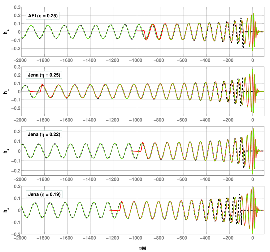
In this paper we use two families of hybrid waveforms. Both are produced by matching 3.5 PN TaylorT1 waveforms with NR waveforms. The first set is constructed by using long ($>10$ inspiral cycles) NR waveforms. This include equal-mass ($\eta=0.25$) NR waveforms produced by the AEI-CCT group using their CCATIE code employing fourth-order finite differencing to compute spatial derivatives, and equal and unequal-mass ($\eta=0.19,0.22,0.25$, or $M_{1}/M_{2}=1,2,3$) waveforms produced by the Jena group using their BAM code employing sixth-order finite differencing and PN-motivated initial-data parameters. The second set of hybrid waveforms is constructed by using NR waveforms produced by the Jena group using their BAM code employing fourth-order finite differencing. These are short waveforms ($\sim 4$ inspiral cycles) densely covering a wide parameter range ($0.16\leq\eta\leq 0.25$). We use the second set of hybrid waveforms to construct the phenomenological family and to test its efficiency in detecting signals from black hole coalescences, and use the first set of hybrid waveforms (which are closer to the actual signals) to verify our results.

The former family of hybrid waveforms is shown in Fig. 2. The NR waveforms from three different simulations ($\eta=0.25,0.22,0.19$) done by AEI and Jena groups are matched with 3.5PN inspiral waveforms over the matching region $-750\leq t/M\leq-550$. The hybrid waveforms are constructed by combining the above as per Eq. (33) and Eq. (39).

The robustness of the matching procedure can be tested by computing the overlaps between hybrid waveforms constructed with different matching regions. If the overlaps are very high, this can be taken as an indication of the robustness of the matching procedure. A preliminary illustration of this can be found in Ref. Ajith (2007), and a more detailed discussion will be presented in Ajith et al. (2007c).

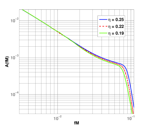
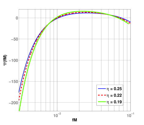
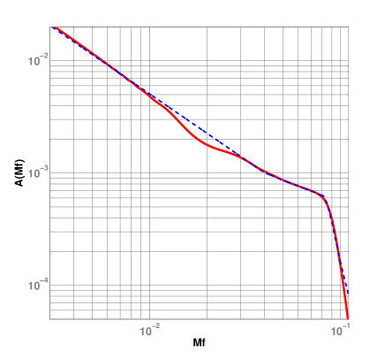
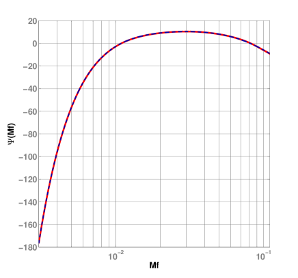
Fig. 3 shows the hybrid waveforms of different mass-ratios in the Fourier domain. In particular, the panel on the left shows the amplitude of the waveforms in the Fourier domain, while the panel on the right shows the phase. These waveforms are constructed by matching 3.5PN waveforms with the long NR waveforms produced by the Jena group. In the next section, we will try to parametrize these Fourier domain waveforms in terms of a set of phenomenological parameters.

Figure 3: Fourier domain magnitude (left) and phase (right) of the (normalized) hybrid waveforms. The constant phase term and the term linear in time (and frequency) have already been subtracted from the phase. Symmetric mass-ratio $\eta$ of each waveform is shown in the legends. These waveforms are constructed by matching 3.5PN waveforms with the long NR waveforms produced by the Jena group.

IV.3 Parametrizing the hybrid waveforms

We propose a phenomenological parametrization to the hybrid waveforms in the Fourier domain. Template waveforms in the Fourier domain are of particular preference because, (i) a search employing Fourier domain templates is computationally inexpensive compared to one using time domain templates (ii) parametrization of the hybrid waveforms is easier in the Fourier domain.

We take our motivation from the restricted post-Newtonian approximation to model the amplitude of the inspiral stage of the hybrid waveform, i.e., the amplitude is approximated to leading order as a power law $f^{-7/6}$ in terms of the Fourier frequency $f$ (as follows straight from adding leading order radiation reaction to Newtonian dynamics). The amplitude of the merger stage is empirically approximated as a power law $f^{-2/3}$ (consistent with the observation of Buonanno et al. (2007a)), while the amplitude of the ring down stage is known to be a Lorentzian function around the quasi-normal mode ring down frequency. Similarly, we take our motivation from the stationary phase approximation (see, for example, Thorne (1987)) of the inspiral waveform to write the Fourier domain phase of the hybrid waveform as a series expansion in powers of $f$. As we shall see later, this provides an excellent approximation of the phase of the hybrid waveform.

Figure 4: Fitting factors of the hybrid waveforms with the phenomenological waveform family. Horizontal axis shows the symmetric mass ratio of the binary. Fitting factors are calculated assuming a white noise spectrum, and hence are independent of the mass of the binary.

Figure 5: Hybrid waveforms (solid lines) in the frequency domain, and the ‘best-matched’ phenomenological waveforms (dashed lines). The left panel shows the Fourier domain magnitude, while the right one shows the phase. In the hybrid waveforms, the constant phase term and the term linear in time (and frequency) have already been subtracted from the phase. In the phenomenological waveforms, $t_{0}$ and $\varphi_{0}$ (see Eq.(44)) have been chosen to minimize the phase difference between the hybrid and phenomenological waveforms. These waveforms correspond to a binary with $\eta=0.25$, and are constructed from the ‘short’ NR waveforms produced by the Jena group (see Section IV.2). The ‘dip’ in the left panel at $Mf\simeq 2\times 10^{-2}$ is due to the small eccentricity present in the first few cycles of the NR waveform. All waveforms are normalized assuming a flat noise spectral density.

IV.3.1 Phenomenological waveforms

We write our phenomenological waveform in the Fourier domain as

$$u(f)\equiv{A}_{\rm eff}(f)\,e^{{\mathrm{i}}\Psi_{\rm eff}(f)}.$$ (40)

where ${A}_{\rm eff}(f)$ is the amplitude of the waveform in the frequency domain, which we choose to write in terms of a set of ‘amplitude parameters’ $\bm{\alpha}=\{f_{\rm merg},f_{\rm ring},\sigma,f_{\rm cut}\}$ as

$${A_{\rm eff}}(f)\equiv C\left\{\begin{array}[]{ll}\left(f/f_{\rm merg}\right)^{-7/6}&\textrm{if $f<f_{\rm merg}$}\\ \\ \left(f/f_{\rm merg}\right)^{-2/3}&\textrm{if $f_{\rm merg}\leq f<f_{\rm ring}$}\\ \\ w\,{\cal L}(f,f_{\rm ring},\sigma)&\textrm{if $f_{\rm ring}\leq f<f_{\rm cut}$}\end{array}\right.$$ (41)

where $f_{\rm cut}$ is the cutoff frequency of the template and $f_{\rm merg}$ is the frequency at which the power-law changes from $f^{-7/6}$ to $f^{-2/3}$ (as noted previously in Buonanno et al. (2007a) for the equal-mass case). $C$ is a numerical constant whose value depends on the relative orientations of the interferometer and the binary orbit as well as the physical parameters of the binary (see below). Also, in the above expression,

$${\cal L}(f,f_{\rm ring},\sigma)\equiv\left(\frac{1}{2\pi}\right)\frac{\sigma}{(f-f_{\rm ring})^{2}+\sigma^{2}/4}\,,$$ (42)

represents a Lorentzian function of width $\sigma$ centered around $f_{\rm ring}$. The normalization constant $w$ is chosen in such a way that ${A}_{\rm eff}(f)$ is continuous across the ‘transition’ frequency $f_{\rm ring}$, i.e.,

$$w\equiv\frac{\pi\sigma}{2}\left(\frac{f_{\rm ring}}{f_{\rm merg}}\right)^{-2/3}\,.$$ (43)

Taking our motivation from the stationary-phase approximation of the gravitational-wave phase, we write the effective phase $\Psi_{\rm eff}(f)$ as an expansion in powers of $f$,

$$\Psi_{\rm eff}(f)=2\pi ft_{0}+\varphi_{0}+\sum_{k=0}^{7}\psi_{k}\,f^{(k-5)/3}\,,$$ (44)

where $t_{0}$ is the time of arrival, $\varphi_{0}$ is the frequency-domain phase offset, and ${\bm{\psi}}=\{\psi_{0},\,\psi_{2},\,\psi_{3},\,\psi_{4},\,\psi_{6},\,\psi_{7}\}$ are the ‘phase parameters’, that is the set of phenomenological parameters describing the phase of the waveform.

The numerical constant $C$ in Eq. (41) can be determined by comparing the amplitude of the phenomenological waveforms with that of the restricted post-Newtonian waveforms in the frequency domain.

In the restricted post-Newtonian approximation, the Fourier transform of the gravitational signal from an optimally-oriented binary located at an effective distance $d$ can be written as in Eq. (67). We expect that in the inspiral stage ($f<f_{\rm merg}$) of our phenomenological waveforms the amplitude will be equal to that of the post-Newtonian waveforms as given in Eq. (67). Thus, in the case of an optimally-oriented binary, the numerical constant $C$ can be computed as

$$C=\frac{M^{5/6}\,f_{\rm merg}^{-7/6}}{d\,\pi^{2/3}}\left(\frac{5\,\eta}{24}\right)^{1/2}.$$ (45)

This ‘physical’ scaling will be useful when we estimate the sensitivity of a search using this template family (see Section IV.6 and Appendix B).

We now compute the fitting factors of the hybrid waveforms with the family of phenomenological waveforms by maximizing the overlaps over all the parameters, i.e., $\{{\bm{\alpha}},{\bm{\psi}},\varphi_{0},t_{0}\}$ of the phenomenological waveforms. While doing this, we also find the parameters, ${\bm{\alpha}}_{\max}$ and ${\bm{\psi}}_{\max}$, of the ‘best-matched’ phenomenological waveforms. This calculation is described in detail in Appendix A.

We first take a few (seven) hybrid waveforms coarsely spaced in the parameter range $0.16\leq\eta\leq 0.25$, and compute the fitting factors and the best-matched phenomenological parameters, assuming a white-noise spectrum for the detector noise. We use these samples in the parameter space to construct the interpolated template bank (see next subsection). We then test the effectualness and faithfulness of the template bank using all ($\sim$ 30) hybrid waveforms finely spaced in the parameter space.

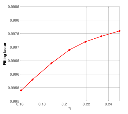
The fitting factors are shown in Fig. 4. It is quite apparent that the fitting factors are always greater than 0.99, thus underlining the effectiveness of the phenomenological waveforms in reproducing the hybrid ones. Also, as an example, in Fig. 5, we plot the hybrid waveforms from $\eta=0.25$ binary in Fourier domain along with the ‘best-matched’ phenomenological waveform.

IV.3.2 From phenomenological to physical parameters

Figure 6: Best-matched amplitude parameters ${{\bm{\alpha}}}_{\rm max}$ in terms of the physical parameters of the binary (assuming white noise spectrum). The horizontal axis shows the symmetric mass-ratio of the binary. Quadratic polynomial fits ${{\bm{\alpha}}}_{\rm int}$ to the data points are also shown.

Figure 7: Best-matched phase parameters ${{\bm{\psi}}}_{\rm max}$ in terms of the physical parameters of the binary (assuming white noise spectrum). The horizontal axis shows the symmetric mass-ratio of the binary. Quadratic polynomial fits ${{\bm{\psi}}}_{\rm int}$ to the data points are also shown.

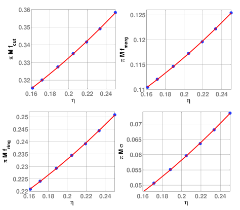
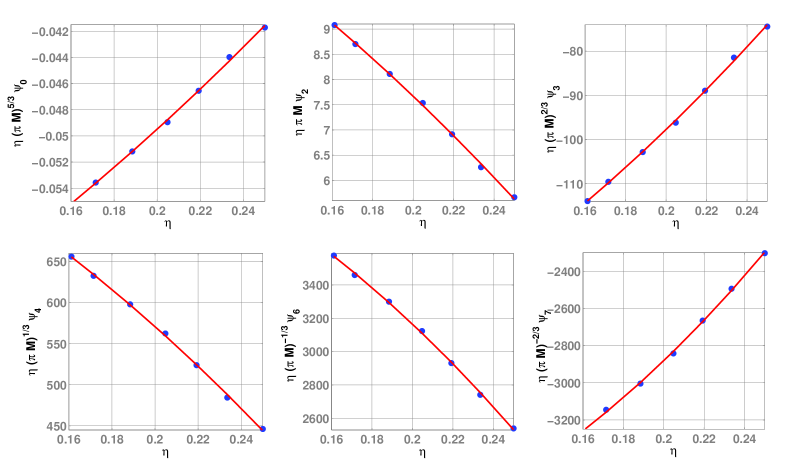
It is possible to parametrize the phenomenological waveforms having the largest overlaps with the hybrid waveforms in terms of the physical parameters of the hybrid waveforms. In Fig. 6, we plot the amplitude parameters ${\bm{\alpha}}_{\rm max}$ of the best-matched phenomenological waveforms against the physical parameters of the binary. Similarly, the phase parameters ${{\bm{\psi}}}_{\rm max}$ of the best-matched phenomenological waveforms are plotted against the physical parameters of the binary in Fig. 7.

It can be seen that ${\bm{\alpha}}_{\rm max}$ and ${\bm{\psi}}_{\rm max}$ can be written as quadratic polynomials in terms of the physical parameters ($M$ and $\eta$) of the hybrid waveforms as:

$$\alpha_{j~{}\rm int} = \frac{a_{j}\,\eta^{2}+b_{j}\,\eta+c_{j}}{\pi M}\,,$$

$$\psi_{k~{}\rm int} = \frac{x_{k}\,\eta^{2}+y_{k}\,\eta+z_{k}}{\eta\,(\pi M)^{(5-k)/3}}\,,$$ (46)

where $a_{j},\,b_{j},\,c_{j},~{}j=0...3$ and $x_{k},\,y_{k},\,z_{k},~{}k=0,\,2,\,3,\,4,\,6,\,7$ are the coefficients of the quadratic polynomials used to fit the data given in Figs. 6 and 7. These coefficients are listed in Tables 1 and 2. It may be noted at this point that Figs. 6 and 7 correspond to the mapping $P:{\bm{\theta}}^{(n)}\rightarrow{\bm{\lambda}}_{\max}^{(n)}$ that we have introduced in Section IV.1, and Eq. (46) to the interpolation $P_{\rm int}$ of $P$.

Using the empirical relations given in Eq. (46), we can rewrite the effective amplitude and phase of the waveforms in terms of $M$ and $\eta$ as:

$${A_{\rm eff}}(f) \equiv C\,\left\{\begin{array}[]{ll}\left(\frac{\pi Mf}{a_{0}\eta^{2}+b_{0}\eta+c_{0}}\right)^{-7/6}&\textrm{if~{}~{}$f<\frac{a_{0}\eta^{2}+b_{0}\eta+c_{0}}{\pi M}$}\\ \\ \left(\frac{\pi Mf}{a_{0}\eta^{2}+b_{0}\eta+c_{0}}\right)^{-2/3}&\textrm{if~{}~{}$\frac{a_{0}\eta^{2}+b_{0}\eta+c_{0}}{\pi M}\leq f<\frac{a_{1}\eta^{2}+b_{1}\eta+c_{1}}{\pi M}$}\\ \\ w\,{\cal L}\left(f,\,\frac{a_{1}\eta^{2}+b_{1}\eta+c_{1}}{\pi M},\,\frac{a_{2}\eta^{2}+b_{2}\eta+c_{2}}{\pi M}\right)&\textrm{if~{}~{}$\frac{a_{1}\eta^{2}+b_{1}\eta+c_{1}}{\pi M}\leq f<\frac{a_{3}\eta^{2}+b_{3}\eta+c_{3}}{\pi M}$}\,,\\ \end{array}\right.$$

$$\Psi_{\rm eff}(f) = 2\pi ft_{0}+\varphi_{0}+\frac{1}{\eta}\,\sum_{k=0}^{7}(x_{k}\,\eta^{2}+y_{k}\,\eta+z_{k})\,(\pi Mf)^{(k-5)/3}\,,$$ (48)

where the constant $C$ is given by Eq.(45). We use this family of parametrized waveforms to create a two-dimensional template bank of non-spinning waveforms. This template family can be seen as a two-dimensional sub-manifold (parametrized by $M$ and $\eta$) embedded in a higher dimensional manifold (of the phenomenological waveforms).

The polynomial coefficients in the Table 2 are indeed significantly different from those predicted by stationary phase approximation of the PN inspiral phase in the frequency domain. There are two reasons for that: The first one is that our re-parametrization is optimized for the mass range where all three phases (inspiral, merger and ring down) are contributing significantly. The second reason is the residual eccentricity present in the numerical waveforms. Change in the relative significance of different PN terms reflects attempt to match the slightly eccentric waveform with circular. When more accurate (less eccentric) numerical waveforms become available in future, the re-parametrization given in Eq.(46) can be optimized for a wider mass range. An example of this can be seen in Ref. Ajith (2007).

IV.4 Effectualness and faithfulness

In order to measure the accuracy of our parametrized templates we compute their overlap with the ‘target signals’ (the hybrid waveform). To check the faithfulness of our phenomenological templates, we compute their overlap with the target signal maximizing it over the extrinsic parameters (time-of-arrival and the initial phase). We assess the effectualness of the parametrized waveforms by computing fitting factors with the target signals (computing the overlap maximized over both extrinsic and intrinsic parameters). Faithfulness is a measure of how good the template waveform is in both detecting a signal and estimating its parameters. However, effectualness is aimed at finding whether or not an approximate template model is good enough in detecting a signal without reference to its use in estimating the parameters.

We compute the effectualness and the faithfulness of the template family for three different noise spectra. The one-sided noise power spectral density (PSD) of the Initial LIGO detector is given in terms of a dimensionless frequency $x=f/f_{0}$ by LAL

$$S_{h}(f)=9\times 10^{-46}\left[(4.49x)^{-56}+0.16x^{-4.52}+0.52+0.32x^{2}\right]\,,$$ (49)

where $f_{0}=150$ Hz; while the same for Virgo reads LAL

$$S_{h}(f)=10.2\times 10^{-46}\left[(7.87x)^{-4.8}+6/17x^{-1}+1+x^{2}\right]\,,$$ (50)

where $f_{0}=500$ Hz. For Advanced LIGO LAL ,

$$S_{h}(f)=10^{-49}\left[x^{-4.14}-5x^{-2}+111\Big{(}\frac{1-x^{2}+x^{4}/2}{1+x^{2}/2}\Big{)}\right]\,,$$ (51)

where $f_{0}=215$ Hz.

Faithfulness is computed by maximizing the overlaps over the extrinsic parameters $t_{0}$ and $\varphi_{0}$ only, which can be done trivially Schutz (1991). Effectualness is computed by maximizing both intrinsic and extrinsic parameters of the binary. The maximization over the intrinsic parameters is performed with the aid of the Nelder-Mead downhill simplex algorithm Nelder and Mead (1964).

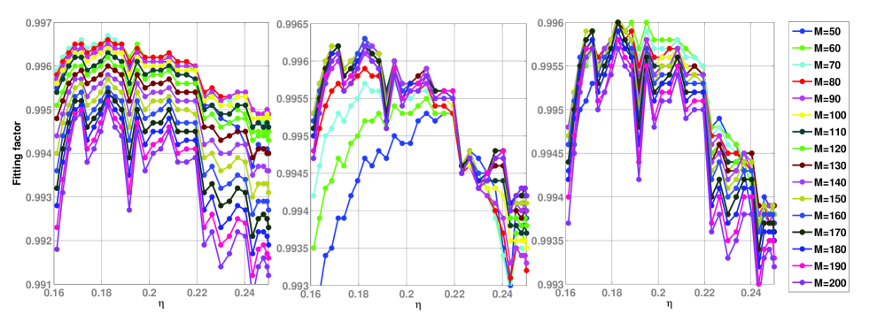
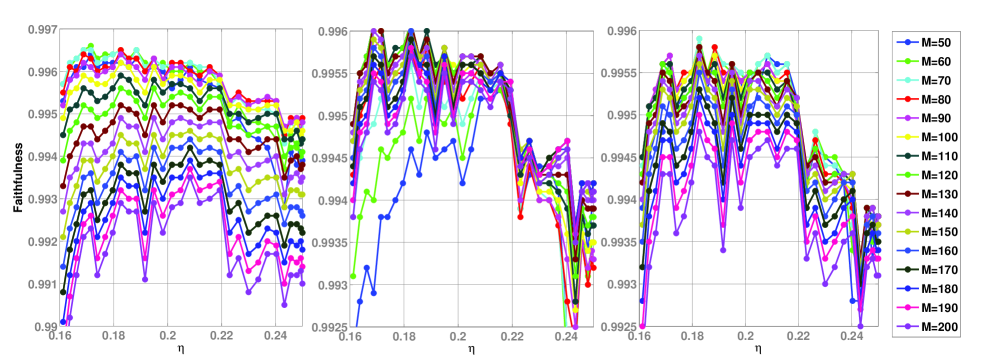
The effectualness of the template waveforms with the hybrid waveforms is plotted in Fig. 8 for three different noise spectral densities. The corresponding faithfulness is plotted in Fig. 9. It is evident that, having both values always greater than 0.99, the proposed template family is both effectual and faithful.

We also calculate the systematic bias in the estimation of parameters while maximizing the overlaps over the intrinsic parameters of the binary. The bias in the estimation of the parameters ${\bm{\theta}}$ is defined in Eq.(30).

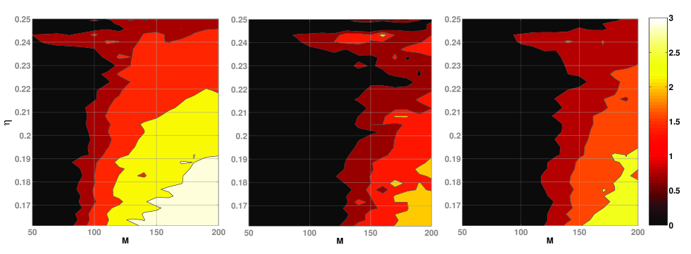
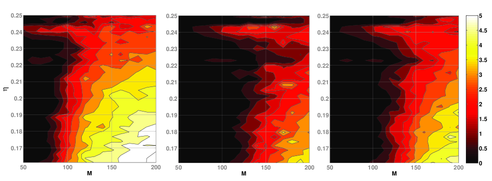
The percentage biases in estimating the total mass $M$, mass ratio $\eta$, and chirp mass $M_{\rm c}=M\eta^{3/5}$ of the binary are plotted in Figs. 10, 11, and 12, respectively. This preliminary investigation suggests that the bias in the estimation of $M$ and $\eta$ using the proposed template family is $<3\%$, while the same in estimating $M_{\rm c}$ is $<6\%$.

Parameter	$a_{k}$	$b_{k}$	$c_{k}$
$f_{\rm merg}$	2.9740$\times 10^{-1}$	4.4810$\times 10^{-2}$	9.5560$\times 10^{-2}$
$f_{\rm ring}$	5.9411$\times 10^{-1}$	8.9794$\times 10^{-2}$	1.9111$\times 10^{-1}$
$\sigma$	5.0801$\times 10^{-1}$	7.7515$\times 10^{-2}$	2.2369$\times 10^{-2}$
$f_{\rm cut}$	8.4845$\times 10^{-1}$	1.2848$\times 10^{-1}$	2.7299$\times 10^{-1}$

Table 1: Polynomial coefficients of the best-matched amplitude parameters. The first column lists the amplitude parameters ${\bm{\alpha}}_{\rm int}$. Eq.(46) shows how these parameters are related to the coefficients $a_{k},b_{k},c_{k}$.

Parameter	$x_{k}$	$y_{k}$	$z_{k}$
$\psi_{0}$	1.7516$\times 10^{-1}$	7.9483$\times 10^{-2}$	-7.2390$\times 10^{-2}$
$\psi_{2}$	-5.1571$\times 10^{1}$	-1.7595$\times 10^{1}$	1.3253$\times 10^{1}$
$\psi_{3}$	6.5866$\times 10^{2}$	1.7803$\times 10^{2}$	-1.5972$\times 10^{2}$
$\psi_{4}$	-3.9031$\times 10^{3}$	-7.7493$\times 10^{2}$	8.8195$\times 10^{2}$
$\psi_{6}$	-2.4874$\times 10^{4}$	-1.4892$\times 10^{3}$	4.4588$\times 10^{3}$
$\psi_{7}$	2.5196$\times 10^{4}$	3.3970$\times 10^{2}$	-3.9573$\times 10^{3}$

Table 2: Polynomial coefficients of the best-matched phase parameters. The first column lists the phase parameters ${\bm{\psi}}_{\rm int}$. Eq.(46) shows how these parameters are related to the coefficients $x_{k},y_{k},z_{k}$.

Figure 8: Fitting factor of the (two-dimensional) template family computed using three different noise spectra. The panel in the left correspond to the Initial LIGO noise PSD, the one in the middle to the Virgo noise PSD and the one in the right to the Advanced LIGO noise PSD. The horizontal axis represents the symmetric mass ratio $\eta$ of the binary and the legends display the total mass $M$ (in units of $M_{\odot}$).

Figure 9: Same as in Fig. 8, except that the plots show the faithfulness of the (two-dimensional) template family.

Figure 10: Bias in the estimation of $M$. Horizontal axis reports the total mass $M$ (in units of $M_{\odot}$) and vertical axis reports the symmetric mass ratio $\eta$ of the binary. Colors in the plot corresponds to the percentage bias, $|\Delta M|/M\times 100$. The left panel corresponds to the Initial LIGO noise PSD, the middle panel to the Virgo noise PSD and the right panel to the Advanced LIGO noise PSD.

Figure 11: Same as in Fig. 10, except that the plots show the percentage bias $|\Delta\eta|/\eta\times 100$ in the estimation of $\eta$.

Figure 12: Same as in Fig. 10, except that the plots show the percentage bias $|\Delta M_{\rm c}|/M_{\rm c}\times 100$ in the estimation of $M_{\rm c}=M\eta^{3/5}$.

IV.5 Verification of the results using more accurate hybrid waveforms

As we have discussed in Section IV.2, the hybrid waveforms used for constructing the template waveforms are produced by matching rather short ($\sim$ 4 inspiral cycles) NR waveforms with PN waveforms. We have also produced a few hybrid waveforms by matching PN waveforms with long ($>$ 10 inspiral cycles) and highly accurate (sixth-order finite differencing and low eccentricity) NR waveforms. This set of hybrid waveforms (which are closer to the ‘actual signals’) can be used to verify the efficacy of the template waveforms in reproducing these more accurate signals.

Fig. 13 shows the fitting factors of the two-dimensional template family with the ‘more accurate’ hybrid waveforms. The fitting factors are computed, as before, using the Initial LIGO (left), Virgo (middle) and Advanced LIGO (right) noise spectra. The high fitting factors (although smaller than the same obtained in the previous Section) with the hybrid waveforms once again underline the efficacy of the template waveforms in reproducing the hybrid ones. It is indeed expected that the template family will have better overlaps with the hybrid waveforms described in the previous Section (those constructed from ‘short’ NR waveforms), because the polynomial coefficients given in Tables 1 and 2 are optimized for these hybrid waveforms. When more ‘long and accurate’ NR waveforms are available in the future, the polynomial coefficients given in the Tables can be optimized for the corresponding family of ‘more accurate’ hybrid waveforms. In any case, since the fitting factors are already very high, we don’t expect any significant improvements.

Figure 13: Fitting factor of the (two-dimensional) template family with ‘more accurate’ hybrid waveforms (see Section IV.5). The overlaps are computed using three different noise spectra. The panel in the left correspond to the Initial LIGO PSD, the one in the middle to the Virgo noise PSD and the one in the right to the Advanced LIGO noise PSD. The horizontal axis represents the total mass $M$ (in units of $M_{\odot}$) and the legends display the symmetric mass ratio $\eta$ of the binary.

IV.6 The astrophysical range and comparison with other searches

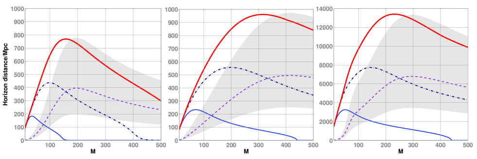
The template family proposed in this paper can be used for coherently searching for all the three stages (inspiral, merger, and ring-down) of the binary black hole coalescence, thus making this potentially more sensitive than searches which look at the three stages separately. Fig. 14 compares the sensitivity of the searches using different template families. What is plotted here are the distances at which an optimally-oriented, equal-mass binary would produce an optimal SNR of 8 at the Initial LIGO (left plot), Virgo (middle plot) and Advanced LIGO (right plot) noise spectra. In each plot, the thin solid (blue) line corresponds to a search using PN templates truncated at the innermost stable circular orbit (ISCO) of the Schwarzschild geometry having the same mass as the total mass $M$ of the binary; the dashed (purple) line to a search using ring-down templates Goggin (2006); the dot-dashed (black) line to a search using effective one body Buonanno and Damour (1999) waveform templates truncated at the light ring of the corresponding Schwarzschild geometry, and the solid line to a search using all three stages of the binary coalescence using the template bank proposed here. The computation is described in detail in Appendix B. The horizontal axis reports the total-mass of the binary, while the vertical axis the distance in Mpc. It is quite evident that, for a substantial range of total mass ($100\lesssim M/M_{\odot}\lesssim 300$ for Initial LIGO, $200\lesssim M/M_{\odot}\lesssim 500$ for Virgo, $150\lesssim M/M_{\odot}\lesssim 400$ for Advanced LIGO), the ‘coherent search’ using the new template family is significantly more sensitive than any other search considered here.

However, while this looks promising, we repeat here the caveats emphasized in Ajith et al. (2007a): It is important to treat Fig. 14 as only a preliminary assessment; fitting factors are not the only consideration for a practical search strategy. It is also very important to consider issues which arise when dealing with real data. For example, false alarms produced by noise artifacts might well determine the true sensitivity of the search, and these artifacts will inevitably be present in real data. This is however beyond the scope of the present work, and further investigation is required before we can properly assess the efficacy of our phenomenological template bank in real-life searches.

Figure 14: Distance to optimally located and oriented equal-mass binaries which can produce an optimal SNR of 8 at the Initial LIGO (left plot), Virgo (middle plot) and Advanced LIGO (right plot) noise spectra. Horizontal axis reports the total mass of the binary (in units of $M_{\odot}$) and vertical axis reports the distance in Mpc. In each plot, the thin solid (blue) line corresponds to a search using standard PN templates truncated at ISCO, the dotted-dashed (black) line to a search using effective one body waveform templates truncated at the light ring, the the dashed (purple) line to a search using ring-down templates, and the thick solid (red) line to a search using the template family proposed in this paper. The ring down horizon distance is computed assuming that $\epsilon=0.7\%$ of the black hole mass is radiated in the ring down stage, while the Kerr parameter $a=0.69$ is known from the numerical simulation. Since the value of $\epsilon$ has some amount of uncertainty in it, we have also included the shaded region in the plot corresponding to $0.18\%\leq\epsilon\leq 2.7\%$.

V Summary and outlook

Making use of the recent results from numerical relativity we have proposed a phenomenological waveform family which can model the inspiral, merger and ring-down stages of the coalescence of non-spinning binary black holes in quasi-circular orbits. We first constructed a set of hybrid waveforms by matching the NR waveforms with analytical PN waveforms. Then, we constructed analytical phenomenological waveforms which approximated the hybrid waveforms. The family of phenomenological waveforms that we propose was found to have fitting factors larger than 0.99 with the hybrid waveforms. We have also shown how this phenomenological waveform family can be parametrized solely in terms of the physical parameters ($M$ and $\eta$) of the binary, so that the template bank is, in the end, two dimensional . This two dimensional template family can be explicitly expressed in terms of the physical parameters of the binary. We have estimated the ‘closeness’ of this two-dimensional template family with the family of hybrid waveforms in the detection band of three ground-based GW detectors, namely Initial LIGO, Virgo and Advanced LIGO. We have estimated the effectualness (larger overlaps with the target signals for the purpose of detection) and faithfulness (smaller biases in the estimation of the parameters of the target signals) of the template family. Having both types of overlap always greater than 0.99, the two dimensional template family is found to be both effectual and faithful in the detection band of these ground-based detectors.

This phenomenological waveform family can be used to densely cover the parameter space, avoiding the computational cost of generating numerical waveforms at every grid point in the parameter space. We have compared the sensitivity of a search using this template family with other searches. For a substantial mass-range, the search using all three stages of the binary black hole coalescence was found to be significantly more sensitive than any other template-based searches considered in this paper. This might enable us to do a more sensitive search for intermediate-mass black holes using ground-based GW detectors.

A number of practical issues need to be addressed before we can employ this template family in an actual search for GW signatures. The first issue will be how to construct a bank of templates sufficiently densely spaced in the parameter space so that the loss in the event rate because of the mismatch between the signal and template is restricted to an acceptable amount (say, 10%). The explicit frequency domain parametrization of the proposed template family makes it easier to adopt the formalism proposed by Owen Owen (1996) in laying down the templates using a metric in the parameter space. Work is ongoing to compare the metric formalism adopted to the proposed template family and other ways of laying out the templates, for example a ‘stochastic’ template bank Allen and Sathyaprakash . Also, this explicit parametrization makes it easier to employ additional signal-based vetoes, such as the ‘chi-square test’ Allen (2005). This will also be explored in a forthcoming work.

Since this template bank is also a faithful representation of the target signals considered, we expect that, for a certain mass-range, a search which coherently includes all three stages of the binary coalescence will bring about remarkable improvement in the estimation of parameters of the binary. This may be especially important for LISA data analysis in estimating the parameters of supermassive black hole binaries. This is also being explored in an ongoing work Ajith et al. (2007b).

It is worth pointing out that the family of target signals (the hybrid waveforms) that we have considered in this paper is not unique. One can construct alternate families of hybrid waveforms by matching PN waveforms computed using different approximations with NR waveforms. Also, owing to the differences in initial data and accuracy of numerical techniques, the NR waveforms from different simulations can also be slightly different. Thus, the coefficients listed in Tables 1 and 2 have a unique meaning only related to this particular family of target waveforms. But we expect that the general parametrization that we propose in this paper will hold for the whole family of non-spinning black hole coalescence waveforms from quasi-circular inspiral. As we have mentioned in the Introduction, the purpose of this paper is to explicitly prescribe a general procedure to construct interpolated template banks using parametrized waveforms which mimics actual signals from binary black hole coalescence (as predicted by numerical relativity and analytical methods).

Nevertheless, it may be noted that most of the PN waveforms constructed using different approximations are known to be very close to each other (see, for example, Damour et al. (2001a)). Also, we expect that NR waveforms from different simulations will converge as the accuracy of numerical simulations improves (see, for example, Baker et al. (2007)). Thus, since different families of PN and NR waveforms, which are the ‘ingredients’ for constructing our target signals, are very close to each other, we expect that the phenomenological waveform family proposed in this paper, in its present form, will be sufficiently close to other families of target signals for the purpose of detecting these signals. As a preliminary illustration of this, we have computed the fitting factors of the template waveforms with a different family of hybrid waveforms (constructed from longer and more accurate NR waveforms), and have shown that the overlaps are indeed very high. This will be explored in detail in a forthcoming work.

Also, we remind the reader that this paper consider only the leading harmonic of the GW signal ($\ell=2,\ m=\pm 2$). We expect that the contribution from the higher harmonics become important for high mass ratios, which will be investigated in a forthcoming work.

Appendix A Calculation of the fitting factors

In order to find the fitting factor of our phenomenological bank to a hybrid waveform, as well as the best-matched parameters $({\bm{\alpha}}_{\rm max},{\bm{\psi}}_{\rm max})$, we need to perform a maximization of the overlap $\mathcal{M}({\bm{\alpha}},{\bm{\psi}})$ in a 12-dimensional space, which seems a challenging task at first sight, especially due to the oscillatory nature of the dependence of $\mathcal{M}({\bm{\alpha}},{\bm{\psi}})$ on the components of ${\bm{\psi}}$. However, due to the very high fitting factor, as well as the linear dependence of $\Psi_{\rm eff}({\bm{\psi}};f)$ on ${\bm{\psi}}$, we have been able to design an analytic approximation to $\mathcal{M}({\bm{\alpha}},{\bm{\psi}})$ that is highly accurate and can be maximized over ${\bm{\psi}}$ analytically. In describing this approximation, we also include $\varphi_{0}$ and $t_{0}$ in ${\bm{\psi}}$, forming an 8-dimensional vector.

For a target hybrid waveform

$$\tilde{h}(f)=A(f)\,e^{{\rm i}\Psi(f)}\,,$$ (52)

and a phenomenological template

$$u(f)=A_{\rm eff}({{\bm{\alpha}};f})\,e^{{\rm i}\Psi_{\rm eff}({\bm{\psi}};f)}\,,$$ (53)

the overlap $\mathcal{M}({\bm{\alpha}},{\bm{\psi}})$ can be broken into a product of two terms,

$$\mathcal{M}({\bm{\alpha}},{\bm{\psi}})=\mathcal{M}_{\rm A}({\bm{\alpha}})\,\mathcal{M}_{\rm P}({\bm{\alpha}},{\bm{\psi}})$$ (54)

with

$$\mathcal{M}_{\rm A}({\bm{\alpha}})\equiv\frac{1}{a}{\int_{0}^{\infty}\frac{A_{\rm eff}({\bm{\alpha}};f)A(f)}{S_{h}(f)}{\rm d}f}$$ (55)

and

$$\mathcal{M}_{\rm P}({\bm{\alpha}},{\bm{\psi}})\equiv\frac{1}{b}\int_{0}^{\infty}\frac{A_{\rm eff}({\bm{\alpha}};f)A(f)\cos[\Delta\Psi(f)]}{S_{h}(f)}{\rm d}f$$ (56)

where

$$\Delta\Psi(f)\equiv\Psi(f)-\Psi_{\rm eff}({\bm{\psi}};f)\,.$$ (57)

In the above expressions, the normalization constants $a$ and $b$ are defined by

$$a^{2}\equiv{\int_{0}^{\infty}\frac{A^{2}(f)}{S_{h}(f)}{\rm d}f\int_{0}^{\infty}\frac{A_{\rm eff}^{2}({\bm{\alpha}};f)}{S_{h}(f)}}{\rm d}f,$$ (58)

and

$$b\equiv{\int_{0}^{\infty}\frac{A_{\rm eff}({\bm{\alpha}};f)A(f)}{S_{h}(f)}{\rm d}f}\,.$$ (59)

If the phase difference $\Delta\Psi(f)$ is small, we can approximate $\cos\Delta\Psi\approx 1-\Delta\Psi^{2}/2$, and rewrite $\mathcal{M}_{\rm P}$ as

$$\mathcal{M}_{\rm P}\approx\mathcal{M}_{\rm P}^{\prime}\equiv 1-\frac{1}{2\,b}\int_{0}^{\infty}\frac{A_{\rm eff}({\bm{\alpha}};f)A(f)[\Delta\Psi(f)]^{2}}{S_{h}(f)}{\rm d}f.$$ (60)

Since $\Psi_{\rm eff}({\bm{\psi}};f)$ is a linear function in ${\bm{\psi}}$, minimizing $\mathcal{M}^{\prime}_{\rm P}$ becomes a least-square fit with a weighting function

$$\mu(f)\equiv\frac{A_{\rm eff}({\bm{\alpha}};f)A(f)}{S_{h}(f)}.$$ (61)

More specifically, writing $\Psi_{\rm eff}({\bm{\psi}};f)$ as in Eq.(44), i.e.,

$$\Psi_{\rm eff}({\bm{\psi}};f)=\sum_{j}\psi_{j}\,f^{(5-j)/3}\,,$$ (62)

we have

$$1-\mathcal{M}^{\prime}_{\rm P}=\frac{1}{2}\left[{\bm{\psi}}\,{\sf A}\,{\bm{\psi}}^{\rm T}-2\,{\bf B}\,{\bm{\psi}}^{\rm T}+D\right]\,,$$ (63)

where we have defined a matrix ${\sf A}$, a vector ${\bf B}$ and a scalar constant $D$, such that

$$A_{ij} \equiv \frac{1}{b}{\int_{0}^{\infty}f^{(10-i-j)/3}\,\mu(f)\,{\rm d}f}\,,$$

$$B_{j} \equiv \frac{1}{b}{\int_{0}^{\infty}f^{(5-j)/3}\Psi(f)\,\mu(f)\,{\rm d}f}\,,$$

$$D \equiv \frac{1}{b}{\int_{0}^{\infty}\Psi^{2}(f)\,\mu(f)\,{\rm d}f}\,.$$ (64)

The maximum of $\mathcal{M}^{\prime}_{\rm P}$ is then equal to

$$\mathcal{M}^{\prime}_{\rm P\,max}=1-\frac{1}{2}\left[D-{\bf B}\,{\sf A}^{-1}\,{\bf B}\right]\,,$$ (65)

reached at

$${\bm{\psi}}_{\rm max}={\bf B}\,{\sf A}^{-1}.$$ (66)

As a consequence, for each ${\bm{\alpha}}$, we are able to maximize $\mathcal{M}_{\rm P}({\bm{\alpha}},{\bm{\psi}})$, and hence $\mathcal{M}({\bm{\alpha}},{\bm{\psi}})$, over ${\bm{\psi}}$ analytically. The original 12-dimensional maximization is then converted to a 4-dimensional maximization, only over the amplitude parameters, on which the overlap depends in a non-oscillatory way.

Appendix B Computing the horizon distance

Here we describe how we compute the horizon distance of different searches discussed in Section IV.6. An alternative way of computing the horizon distance can be found in Ref. Ajith (2007).

B.1 Search using post-Newtonian templates

In the restricted post-Newtonian approximation, the Fourier transform of the gravitational signal from an optimally-oriented binary located at an effective distance $d$ can be written in the following way:

$$h(f)=\frac{M^{5/6}}{d\,\pi^{2/3}}\left(\frac{5\,\eta}{24}\right)^{1/2}\,f^{-7/6}\,e^{{\rm i}[2\pi ft_{0}-\varphi_{0}+\psi(f)-\pi/4]}$$ (67)

where $M$ is the total mass, $\eta$ is the symmetric mass ratio, $t_{0}$ is the time of arrival and $\varphi_{0}$ is the initial phase. The phase $\psi(f)$ is computed using the stationary phase approximation.

The optimal SNR in detecting a known signal $h$ buried in the noise is given by

$$\rho_{\rm opt}=2\left[\int_{0}^{\infty}{\rm d}f\,\frac{h(f)^{2}}{S_{h}(f)}\right]^{1/2},$$ (68)

where $S_{h}(f)$ is the one-sided PSD of the noise. The optimal SNR in detecting the signal given in Eq.(67) can thus be computed as:

$$\rho_{\rm opt}=\frac{M^{5/6}}{d\,\pi^{2/3}}\left(\frac{5\,\eta}{6}\right)^{1/2}\left[\int_{f_{\rm low}}^{f_{\rm upp}}{\rm d}f\frac{f^{-7/3}}{S_{h}(f)}\right]^{1/2}\,,$$ (69)

where $f_{\rm low}$ is the low-frequency cutoff of the detector noise and $f_{\rm upp}$ is upper frequency cutoff of the template waveform. The effective distance to a binary which can produce an optimal SNR $\rho_{\rm opt}$ can be computed by inverting the above equation.

The standard post-Newtonian waveforms are truncated at $f_{\rm upp}=f_{\rm ISCO}$, where $f_{\rm ISCO}=(6^{3/2}\pi M)^{-1}$ is the GW frequency corresponding to the innermost stable circular orbit (ISCO) of the Schwarzschild geometry with mass equal to the total mass $M$ of the binary. The effective one body (EOB) waveforms are truncated at $f_{\rm upp}=f_{\rm LR}$, where $f_{\rm LR}=(3^{3/2}\pi M)^{-1}$ is the GW frequency corresponding to the light ring of the Schwarzschild geometry with mass $M$. Both of these quantities are computed assuming the test particle limit. It may be noted that, for the EOB waveforms, an analytical Fourier domain representation is not available. They cannot be expressed in the form given in Eq.(67). But for the purpose of the estimation of the horizon distance, these formulas give a reasonable approximation.

B.2 Search using ring down templates

The ring down portion of the GW signal from a coalescing binary, considering only the fundamental quasi-normal mode, corresponds to a damped sinusoid. This can be written as Echeverria (1989)

$$h_{\rm ring}(t) = A_{\rm ring}\exp\left[-\frac{\pi f_{\textrm{\mbox{\tiny{QNR}}}}(t-t_{0})}{Q}\right]$$ (70)

$$\times\cos\left(-2\pi f_{\textrm{\mbox{\tiny{QNR}}}}(t-t_{0})+\varphi_{0}\right)\,,$$

where $A_{\rm ring}$ is the amplitude, $t_{0}$ is the start time of the ring down, $\varphi_{0}$ the initial phase, $M$ is the mass of final black hole, $f_{\textrm{\mbox{\tiny{QNR}}}}$ and $Q$ are the central frequency and the quality factor of the ringing. For the fundamental mode, a good fit to the frequency $f_{\textrm{\mbox{\tiny{QNR}}}}$ and quality factor $Q$, within an accuracy of 5%, is given by

$$f_{\textrm{\mbox{\tiny{QNR}}}} \approx [1-0.63(1-a)^{3/10}]\frac{1}{2\pi M}\,,$$ (71)

$$Q \approx 2(1-a)^{-9/20}\,,$$ (72)

where $aM^{2}$ is the spin angular momentum, and $a$ is the Kerr parameter Echeverria (1989).

To compute the optimal SNR in detecting this signal present in the data, we proceed as in Flanagan and Hughes (1998b), assuming that for $t<t_{0}$, $h_{\rm ring}(t)$ is identical to $t>t_{0}$ except for the sign in the exponential, and dividing by a correcting factor of $\sqrt{2}$ in amplitude to compensate for the doubling of power:

$$\bar{h}_{\rm ring}(t) = \frac{A_{\rm ring}}{\sqrt{2}}\exp\left[-\frac{\pi f_{\textrm{\mbox{\tiny{QNR}}}}\,|t-t_{0}|}{Q}\right]$$ (73)

$$\times\cos\left(-2\pi f_{\textrm{\mbox{\tiny{QNR}}}}(t-t_{0})+\varphi_{0}\right)\,.$$

Its Fourier transform then becomes

$${\tilde{\bar{h}}}_{\rm ring}(f) = \frac{A_{\rm ring}\,f_{\textrm{\mbox{\tiny{QNR}}}}}{\sqrt{2}\pi\,Q}\,e^{{\rm i}2\pi ft_{0}}\,\left(\frac{e^{{\rm i}\varphi_{0}}}{{g}^{2}+4\,(f-f_{\textrm{\mbox{\tiny{QNR}}}})^{2}}\right.$$ (74)

$$+ \left.\frac{e^{-{\rm i}\varphi_{0}}}{{g}^{2}+4\,(f+f_{\textrm{\mbox{\tiny{QNR}}}})^{2}}\right)\,,$$

where $g=f_{\textrm{\mbox{\tiny{QNR}}}}/Q$.

In general, it is not easy to estimate $A_{\rm ring}$, or the two polarization amplitudes; they depend upon the detailed evolution of the merger epoch, as well as variables such as the orientation of the final merged remnant. A reasonable hypothesis Goggin (2005); Hughes (2002); Fryer et al. (2002) is that their ratio follows the ratio of the inspiral polarization amplitudes. With this hypothesis, the overall amplitude of the signal from an optimally located and oriented binary, requiring that the ring down radiate some fraction $\epsilon$ of the system’s total mass, becomes

$$A_{\rm ring}^{\rm opt}=\sqrt{\frac{5\epsilon}{4\pi}}\frac{M}{d}\frac{2}{\sqrt{Mf_{\textrm{\mbox{\tiny{QNR}}}}QF(Q)}}$$ (75)

where $F(Q)=1+\frac{7}{24Q^{2}}$ and $d$ is the distance to the source. The optimal SNR $\rho$ can now be computed as

$$\rho_{\rm opt}=2\,\left[\int_{f_{\rm low}}^{f_{\rm upp}}{\rm d}f\frac{|{\tilde{\bar{h}}}_{\rm ring}|^{2}}{S_{h}(f)}\right]^{1/2}\,,$$ (76)

where $f_{\rm low}$ and $f_{\rm upp}$ are the lower and upper cutoff frequencies of the detector noise. As in the previous case, the horizon distance can be computed by inverting this equation.

B.3 Search using the template family proposed in this paper

The phenomenological waveforms in the frequency domain are given in Eqs.(40– 45). The optimal SNR in detecting this signal can be computed as:

$$\rho_{\rm opt} = \frac{M^{5/6}\,f_{\rm merg}^{-7/6}}{d\,\pi^{2/3}}\left(\frac{5\,\eta}{6}\right)^{1/2}\left[\int_{f_{\rm low}}^{f_{\rm merg}}{\rm d}f\frac{(f/f_{\rm merg})^{-7/3}}{S_{h}(f)}\right.$$ (77)

$$+ \int_{f_{\rm merg}}^{f_{\rm ring}}{\rm d}f\frac{(f/f_{\rm merg})^{-4/3}}{S_{h}(f)}$$

$$+ w^{2}\left.\int_{f_{\rm ring}}^{f_{\rm cut}}{\rm d}f\frac{{\cal L}^{2}(f,f_{\rm ring},\sigma)}{S_{h}(f)}\right]^{1/2},$$

where ${\cal L}(f,f_{\rm ring},\sigma)$ is defined in Eq.(42), and $f_{\rm merg},f_{\rm ring},f_{\rm cut}$ and $\sigma$ are given by Eq.(46).

This equation can be inverted to calculate the effective distance to the optimally-oriented binary which can produce an optimal SNR $\rho_{\rm opt}$.

References

- Fock (1959) V. Fock, Theory of Space, time and gravitation (Pergamon, London, 1959).
- Blanchet and Damour (1986) L. Blanchet and T. Damour, Phil. Trans. Roy. Soc. Lond. A320, 379 (1986).
- Wagoner and Will (1976) R. V. Wagoner and C. M. Will, Astrophys. J. 210, 764 (1976).
- Damour et al. (1998) T. Damour, B. R. Iyer, and B. S. Sathyaprakash, Phys. Rev. D 57, 885 (1998).
- Buonanno and Damour (1999) A. Buonanno and T. Damour, Phys. Rev. D 59, 084006 (1999), eprint gr-qc/9811091.
- Pretorius (2005) F. Pretorius, Phys. Rev. Lett. 95, 121101 (2005), eprint gr-qc/0507014.
- Campanelli et al. (2006a) M. Campanelli, C. O. Lousto, P. Marronetti, and Y. Zlochower, Phys. Rev. Lett. 96, 111101 (2006a), eprint gr-qc/0511048.
- Baker et al. (2006a) J. G. Baker, J. Centrella, D.-I. Choi, M. Koppitz, and J. van Meter, Phys. Rev. Lett. 96, 111102 (2006a), eprint gr-qc/0511103.
- Herrmann et al. (2007a) F. Herrmann, I. Hinder, D. Shoemaker, and P. Laguna, Class. Quantum Gravity 24, S33 (2007a).
- Sperhake (2006) U. Sperhake (2006), gr-qc/0606079.
- Brügmann et al. (2006) B. Brügmann, J. A. González, M. Hannam, S. Husa, U. Sperhake, and W. Tichy (2006), gr-qc/0610128.
- Thornburg et al. (2007) J. Thornburg, P. Diener, D. Pollney, L. Rezzolla, E. Schnetter, E. Seidel, and R. Takahashi, Class. Quantum Grav. 24, 3911 (2007), eprint gr-qc/0701038.
- Etienne et al. (2007) Z. B. Etienne, J. A. Faber, Y. T. Liu, S. L. Shapiro, and T. W. Baumgarte (2007), eprint arXiv:0707.2083 [gr-qc].
- Baker et al. (2006b) J. G. Baker, J. Centrella, D.-I. Choi, M. Koppitz, J. van Meter, and M. C. Miller, Astrophys. J 653, L93 (2006b), astro-ph/0603204.
- González et al. (2007a) J. A. González, U. Sperhake, B. Brügmann, M. Hannam, and S. Husa, Phys. Rev. Lett. 98, 091101 (2007a), eprint gr-qc/0610154.
- Campanelli et al. (2006b) M. Campanelli, C. O. Lousto, and Y. Zlochower, Phys. Rev. D 74, 041501 (2006b), gr-qc/0604012.
- Campanelli et al. (2006c) M. Campanelli, C. O. Lousto, and Y. Zlochower, Phys. Rev. D 74, 084023 (2006c), gr-qc/0608275.
- Herrmann et al. (2007b) F. Herrmann, I. Hinder, D. Shoemaker, P. Laguna, and R. A. Matzner (2007b), eprint gr-qc/0701143.
- Koppitz et al. (2007) M. Koppitz, D. Pollney, C. Reisswig, L. Rezzolla, J. Thornburg, P. Diener, and E. Schnetter, Phys. Rev. Lett. 99, 041102 (2007), eprint gr-qc/0701163.
- González et al. (2007b) J. A. González, M. D. Hannam, U. Sperhake, B. Brügmann, and S. Husa, Phys. Rev. Lett. 98, 231101 (2007b), eprint gr-qc/0702052.
- Campanelli et al. (2007a) M. Campanelli, C. O. Lousto, Y. Zlochower, and D. Merritt, Astrophys. J. 659, L5 (2007a), eprint gr-qc/0701164.
- Campanelli et al. (2007b) M. Campanelli, C. O. Lousto, Y. Zlochower, B. Krishnan, and D. Merritt, Phys. Rev. D 75, 064030 (2007b), eprint gr-qc/0612076.
- Pollney et al. (2007) D. Pollney, C. Reisswig, L. Rezzolla, B. Szilágyi, M. Ansorg, B. Deris, P. Diener, E. N. Dorband, M. Koppitz, A. Nagar, et al. (2007), eprint arXiv:0707.2559 [gr-qc].
- Rezzolla et al. (2007) L. Rezzolla, E. N. Dorband, C. Reisswig, P. Diener, D. Pollney, E. Schnetter, and B. Szilágy (2007), eprint arXiv:0708.3999 [gr-qc].
- Baker et al. (2006c) J. G. Baker, J. Centrella, D.-I. Choi, M. Koppitz, and J. van Meter, Phys. Rev. D 73, 104002 (2006c), eprint gr-qc/0602026.
- Baker et al. (2006d) J. G. Baker, J. R. van Meter, S. T. McWilliams, J. Centrella, and B. J. Kelly (2006d), eprint gr-qc/0612024.
- Buonanno et al. (2007a) A. Buonanno, G. B. Cook, and F. Pretorius, Phys. Rev. D 75, 124018 (2007a), eprint gr-qc/0610122.
- Berti et al. (2007a) E. Berti et al. (2007a), eprint gr-qc/0703053.
- Pan et al. (2007) Y. Pan et al. (2007), eprint arXiv:0704.1964 [gr-qc].
- Ajith et al. (2007a) P. Ajith et al., Class. Quant. Grav. 24, S689 (2007a), eprint arXiv:0704.3764 [gr-qc].
- Hannam et al. (2007) M. Hannam, S. Husa, U. Sperhake, B. Brügmann, and J. A. González (2007), eprint arXiv:0706.1305 [gr-qc].
- Boyle et al. (2007) M. Boyle et al. (2007), eprint arXiv:0710.0158 [gr-qc].
- Brügmann et al. (2007) B. Brügmann, J. A. Gonzalez, M. Hannam, S. Husa, and U. Sperhake (2007), eprint arXiv:0707.0135 [gr-qc].
- Lousto and Zlochower (2007) C. O. Lousto and Y. Zlochower (2007), eprint arXiv:0708.4048 [gr-qc].
- Scheel et al. (2006) M. A. Scheel, H. P. Pfeiffer, L. Lindblom, L. E. Kidder, O. Rinne, and S. A. Teukolsky, Phys. Rev. D 74, 104006 (2006), eprint gr-qc/0607056.
- Pfeiffer et al. (2007) H. P. Pfeiffer, D. Brown, L. E. Kidder, L. Lindblom, G. Lovelance, and M. A. Scheel (2007), eprint gr-qc/0702106.
- Husa et al. (2007a) S. Husa, J. A. González, M. Hannam, B. Brügmann, and U. Sperhake (2007a), eprint arXiv:0706.0740 [gr-qc].
- Husa et al. (2007b) S. Husa, M. Hannam, J. A. González, U. Sperhake, and B. Brügmann (2007b), eprint arXiv:0706.0904 [gr-qc].
- Buonanno et al. (2007b) A. Buonanno et al. (2007b), eprint arXiv:0706.3732 [gr-qc].
- Berti et al. (2007b) E. Berti, J. Cardoso, V. Cardoso, and M. Cavaglia (2007b), eprint arXiv:0707.1202 [gr-qc].
- Berti et al. (2006) E. Berti, V. Cardoso, and C. M. Will, Phys. Rev. D 73, 064030 (2006), eprint gr-qc/0512160.
- Dreyer et al. (2004) O. Dreyer, B. J. Kelly, B. Krishnan, L. S. Finn, D. Garrison, and R. Lopez-Aleman, Class. Quant. Grav. 21, 787 (2004), eprint gr-qc/0309007.
- Berti et al. (2005) E. Berti, A. Buonanno, and C. M. Will, Class. Quant. Grav. 22, S943 (2005), eprint gr-qc/0504017.
- Flanagan and Hughes (1998a) E. E. Flanagan and S. A. Hughes, Phys. Rev. D 57, 4535 (1998a).
- Buonanno and Damour (2000) A. Buonanno and T. Damour, Phys. Rev. D 62, 064015 (2000), eprint gr-qc/0001013.
- Damour et al. (2001a) T. Damour, B. R. Iyer, and B. S. Sathyaprakash, Phys. Rev. D 63, 044023 (2001a), erratum-ibid. D 72 (2005) 029902, eprint gr-qc/0010009.
- Ajith et al. (2007b) P. Ajith et al. (2007b), in preparation.
- Schutz (1986) B. F. Schutz, Nature (London) 323, 310 (1986).
- Markovic (1993) D. Markovic, Phys. Rev. D48, 4738 (1993).
- Chernoff and Finn (1993) D. Chernoff and L. Finn, Astrophys. J. Lett. 411, L5 (1993).
- Holz and Hughes (2005) D. E. Holz and S. A. Hughes, Astrophys. J 629, 15 (2005), eprint astro-ph/0504616.
- Arun et al. (2007) K. G. Arun, B. R. Iyer, B. S. Sathyaprakash, S. Sinha, and C. V. D. Broeck (2007), eprint arXiv:0707.3920 [astro-ph].
- Blanchet et al. (2004a) L. Blanchet, T. Damour, G. Esposito-Farèse, and B. R. Iyer, Phys. Rev. Lett. 93, 091101 (2004a), eprint gr-qc/0406012.
- Brill and Lindquist (1963) D. R. Brill and R. W. Lindquist, Phys. Rev. 131, 471 (1963).
- Bowen and York (1980) J. M. Bowen and J. W. York, Phys. Rev. D 21, 2047 (1980).
- Brandt and Brügmann (1997) S. Brandt and B. Brügmann, Phys. Rev. Lett. 78, 3606 (1997), eprint gr-qc/9703066.
- Nakamura et al. (1987) T. Nakamura, K. Oohara, and Y. Kojima, Prog. Theor. Phys. Suppl. 90, 1 (1987).
- Shibata and Nakamura (1995) M. Shibata and T. Nakamura, Phys. Rev. D 52, 5428 (1995).
- Baumgarte and Shapiro (1999) T. W. Baumgarte and S. L. Shapiro, Phys. Rev. D 59, 024007 (1999), eprint gr-qc/9810065.
- Bona et al. (1995) C. Bona, J. Massó, E. Seidel, and J. Stela, Phys. Rev. Lett. 75, 600 (1995), eprint gr-qc/9412071.
- Alcubierre et al. (2003) M. Alcubierre, B. Brügmann, P. Diener, M. Koppitz, D. Pollney, E. Seidel, and R. Takahashi, Phys. Rev. D 67, 084023 (2003), eprint gr-qc/0206072.
- Alcubierre and Brügmann (2001) M. Alcubierre and B. Brügmann, Phys. Rev. D 63, 104006 (2001), eprint gr-qc/0008067.
- Hannam et al. (2006) M. Hannam, S. Husa, D. Pollney, B. Brügmann, and N. Ó Murchadha (2006), gr-qc/0606099.
- Schnetter et al. (2006) E. Schnetter, B. Krishnan, and F. Beyer, Phys. Rev. D 74, 024028 (2006), eprint gr-qc/0604015.
- Dennison et al. (2006) K. A. Dennison, T. W. Baumgarte, and H. P. Pfeiffer, Phys. Rev. D74, 064016 (2006), eprint gr-qc/0606037.
- Tichy and Brügmann (2004) W. Tichy and B. Brügmann, Phys. Rev. D 69, 024006 (2004), eprint gr-qc/0307027.
- Cook (1994) G. B. Cook, Phys. Rev. D 50, 5025 (1994).
- Baumgarte (2000) T. W. Baumgarte, Phys. Rev. D 62, 024018 (2000), eprint gr-qc/0004050.
- Newman and Penrose (1962) E. T. Newman and R. Penrose, J. Math. Phys. 3, 566 (1962), erratum in J. Math. Phys. 4, 998 (1963).
- Stewart (1990) J. M. Stewart, Advanced general relativity (Cambridge University Press, Cambridge, 1990).
- Teukolsky (1973) S. A. Teukolsky, Astrophys. J. 185, 635 (1973).
- Nagar and Rezzolla (2005) A. Nagar and L. Rezzolla, Class. Quant. Grav. 22, R167 (2005), eprint gr-qc/0502064.
- Blanchet (2006) L. Blanchet, Living Reviews in Relativity 9 (2006), eprint gr-qc/0202016, URL http://www.livingreviews.org/lrr-2006-4.
- Damour et al. (2000) T. Damour, P. Jaranowski, and G. Schäfer, Phys. Rev. D 62, 044024 (2000).
- Damour et al. (2001b) T. Damour, P. Jaranowski, and G. Schäfer, Phys. Rev. D 63, 044021 (2001b), erratum-ibid 66, 029901(E) (2002).
- Blanchet and Faye (2000) L. Blanchet and G. Faye, Phys. Lett. A 271, 58 (2000), eprint gr-qc/0004009.
- Blanchet and Faye (2001) L. Blanchet and G. Faye, Phys. Rev. D 63, 062005 (2001), eprint gr-qc/0007051.
- de Andrade et al. (2001) V. de Andrade, L. Blanchet, and G. Faye, Class. Quantum Grav. 18, 753 (2001).
- Blanchet et al. (2004b) L. Blanchet, T. Damour, and G. Esposito-Farèse, Phys. Rev. D 69, 124007 (2004b), eprint gr-qc/0311052.
- Itoh and Futamase (2003) Y. Itoh and T. Futamase, Phys. Rev. D 68, 121501(R) (2003).
- Itoh (2004) Y. Itoh, Phys. Rev. D 69, 064018 (2004).
- Blanchet et al. (2002) L. Blanchet, G. Faye, B. R. Iyer, and B. Joguet, Phys. Rev. D 65, 061501(R) (2002), Erratum-ibid 71, 129902(E) (2005), eprint gr-qc/0105099.
- Blanchet (2002) L. Blanchet, Phys. Rev. D 65, 124009 (2002).
- Cutler and Flanagan (1994) C. Cutler and E. E. Flanagan, Phys. Rev. D 49, 2658 (1994), eprint gr-qc/9402014.
- Babak et al. (2006) S. Babak, R. Balasubramanian, D. Churches, T. Cokelaer, and B. S. Sathyaprakash, Class. Quant. Grav. 23, 5477 (2006), eprint gr-qc/0604037.
- Buonanno et al. (2003a) A. Buonanno, Y. Chen, and M. Vallisneri, Phys. Rev. D 67, 024016 (2003a), eprint gr-qc/0205122.
- Buonanno et al. (2003b) A. Buonanno, Y. Chen, and M. Vallisneri, Phys. Rev. D 67, 104025 (2003b), eprint gr-qc/0211087.
- Abbott et al. (2007) B. Abbott et al. (LIGO Scientific Collaboration) (2007), eprint arXiv:0704.3368 [gr-qc].
- Abbott et al. (2006) B. Abbott et al. (LIGO Scientific Collaboration), Phys. Rev. D 73, 062001 (2006), eprint gr-qc/0509129.
- Apostolatos (1995) T. A. Apostolatos, Phys. Rev. D 52, 605 (1995).
- Damour et al. (2003) T. Damour, B. R. Iyer, P. Jaranowski, and B. S. Sathyaprakash, Phys. Rev. D 67, 064028 (2003), eprint gr-qc/0211041.
- Ajith (2007) P. Ajith (2007), eprint arXiv:0712.0343 [gr-qc].
- Ajith et al. (2007c) P. Ajith et al. (2007c), in preparation.
- Thorne (1987) K. Thorne, in Three Hundred Years of Gravitation, edited by S. Hawking and W. Israel (Cambridge University Press, Cambridge, U.K.; New York, U.S.A., 1987), pp. 330–458.
- (95) LSC Algorithms Library, URL http://www.lsc-group.phys.uwm.edu/daswg/projects/lal.html.
- Schutz (1991) B. Schutz, in The Detection of Gravitational Waves, edited by D. Blair (Cambridge University Press, Cambridge, U.K.; New York, U.S.A., 1991), pp. 406–452.
- Nelder and Mead (1964) J. Nelder and R. Mead, The Computer Journal 7, 308 (1964).
- Goggin (2006) L. M. Goggin (LIGO Scientific Collaboration), Class. Quant. Grav. 23, S709 (2006).
- Owen (1996) B. J. Owen, Phys. Rev. D 53, 6749 (1996), eprint gr-qc/9511032.
- (100) B. Allen and B. Sathyaprakash, Private Communication.
- Allen (2005) B. Allen, Phys. Rev. D 71, 062001 (2005), eprint gr-qc/0405045.
- Baker et al. (2007) J. G. Baker, M. Campanelli, F. Pretorius, and Y. Zlochower, Class. Quant. Grav. 24, S25 (2007), eprint gr-qc/0701016.
- Echeverria (1989) F. Echeverria, Phys. Rev. D 40, 3194 (1989).
- Flanagan and Hughes (1998b) E. E. Flanagan and S. A. Hughes, Phys. Rev. D 57, 4535 (1998b), eprint gr-qc/9701039.
- Goggin (2005) L. Goggin (2005), LSC Internal Document.
- Hughes (2002) S. A. Hughes, Mon. Not. Roy. Astron. Soc. 331, 805 (2002), eprint astro-ph/0108483.
- Fryer et al. (2002) C. L. Fryer, D. E. Holz, and S. A. Hughes, Astrophys. J. 565, 430 (2002), eprint astro-ph/0106113.