Abstract

Quality of microarray gene expression data has emerged as a new research topic. As in other areas, microarray quality is assessed by comparing suitable numerical summaries across microarrays, so that outliers and trends can be visualized, and poor quality arrays or variable quality sets of arrays can be identified. Since each single array comprises tens or hundreds of thousands of measurements, the challenge is to find numerical summaries which can be used to make accurate quality calls. To this end, several new quality measures are introduced based on probe level and probeset level information, all obtained as a by-product of the low-level analysis algorithms RMA/fitPLM for Affymetrix GeneChips. Quality landscapes spatially localize chip or hybridization problems. Numerical chip quality measures are derived from the distributions of Normalized Unscaled Standard Errors and of Relative Log Expressions. Quality of chip batches is assessed by Residual Scale Factors. These quality assessment measures are demonstrated on a variety of datasets (spike-in experiments, small lab experiments, multi-site studies). They are compared with Affymetrix’s individual chip quality report.

KEYWORDS: quality control, microarrays, Affymetrix chips, relative log expression, normalized unscaled standard errors, residual scale factors.

1 Introduction

With the introduction of microarrays biologist have been witnessing entire labs shrinking to matchbox size. This paper invites quality researchers to join scientists on their fantastic journey into the world of microscopic high-throughput measurement technologies. Building a biological organism as laid out by the genetic code is a multi-step process with room for variation at each step. The first steps, as described by the Dogma of molecular biology, are genes (and DNA sequence in general), their transcripts and proteins. Substantial factors contributing to their variation in both structure and abundance include cell type, developmental stage, genetic background and environmental conditions. Connecting molecular observations to the state of an organism is a central interest in molecular biology. This includes the study of the gene and protein functions and interactions, and their alteration in response to changes in environmental and developmental conditions. Traditional methods in molecular biology generally work on a ”one gene (or protein) in one experiment” basis. With the invention of microarrays huge numbers of such macromolecules can now be monitored in one experiment. The most common kinds are gene expression microarrays, which measure the mRNA transcript abundance for tens of thousands of genes simultaneously.

For biologists, this high-throughput approach has opened up entirely new avenues of research. Rather than experimentally confirming the hypothesized role of a certain candidate gene in a certain cellular process, they can use genome-wide comparisons to screen for all genes which might be involved in that process. One of the first examples of such an exploratory approach is the expression profiling study of mitotic yeast cells by Cho et al. (1998) which determined a set of a few hundred genes involved in the cell cycle and triggered a cascade of articles re-analyzing the data or replicating the experiment. Microarrays have become a central tool in cancer research initiated by the discovery and re-definition of tumor subtypes based on molecular signatures (see e.g. Perou et al. (2000), Alizadeh et al. (2000), Ramaswamy and Golub (2002), Yeoh et al. (2002)). In Section ?? we will explain different kinds of microarray technologies in more detail and describe their current applications in life sciences research.

A DNA microarray consists of a glass surface with a large number of distinct fragments of DNA called probes attached to it at fixed positions. A fluorescently labelled sample containing a mixture of unknown quantities of DNA molecules called the target is applied to the microarray. Under the right chemical conditions, single-stranded fragments of target DNA will base pair with the probes which are their complements, with great specificity. This reaction is called hybridization, and is the reason DNA microarrays work. The fixed probes are either fragments of DNA called complementary DNA (cDNA) obtained from messenger RNA (mRNA), or short fragments known to be complementary to part of a gene, spotted onto the glass surface, or synthesized in situ. The point of the experiment is to quantify the abundance in the target of DNA complementary to each particular probe, and the hybridization reaction followed by scanning allows this to be done on a very large scale. The raw data produced in a microarray experiment consists of scanned images, where the image intensity in the region of a probe is proportional to the amount of labelled target DNA that base pairs with that probe. In this way we can measure the abundance of thousands of DNA fragments in a target sample. Microarrays based on cDNA or long oligonucleotide probes typically use just one or a few probes per gene. The same probe sequence spotted in different locations, or probe sequences complementary to different parts of the same gene can be used to give within array replication. Short oligonucleotide microarrays typically use a larger number per gene, e.g. 11 for the HU133 Affymetrix array per gene. Such a set of 11 is called probeset for that gene, and the probes in a probe set are arranged randomly over the array. In the biological literature, microarrays are also referred to as (gene) chips or slides.

When the first microarray platforms were introduced in the early 90s, the most intriguing fact about them was the sheer number of genes that could be assayed simultaneously. Assays that used to be done one gene at a time, could suddenly be produced for thousands of genes at once. A decade later, high-density microarrays would even fit entire genomes of higher organisms. After the initial euphoria, the research community became aware that findings based solely on microarray measurements were not always as reproducible as they would have liked and that studies with inconclusive results were quite common. With this high-throughput measurement technology becoming established in many branches of life sciences research, scientists in both academic and corporate environments raised their expectations concerning the validity of the measurements. Data quality issues are now frequently addressed at meetings of the Microarray Gene Expression Database group (MGED). The Microarray Quality Control project, a community-wide effort, under the auspices of the U.S. Food and Drug Administration (FDA), is aiming at establishing operational metrics to objectively assess the performance of seven microarray platform and develop minimal quality standards. Their assessment is based on the performance of a set of standardized external RNA controls. The first formal results of this project have been published in a series of articles in the September 2006 issue of Nature Biotechnology.

Assessing the quality of microarray data has emerged as a new research topic for statisticians. In this paper, we conceptualize microarray data quality issues from a perspective which includes the technology itself as well as their practical use by the research community. We characterize the nature of microarray data from a quality assessment perspective, and we explain the different levels of microarray data quality assessment. Then we focus on short oligonucleotide microarrays to develop a set of specific statistical data quality assessment methods including both numerical measures and spatial diagnostics.

Assumptions and hopes about the quality of the measurements have become a major issue in microarray purchasing. Despite their substantially higher costs, Affymetrix short oligonucleotide microarrays have become a widespread alternative to cDNA chips. Informally, they are considered the industrial standard among all microarray platforms. More recently, Agilent’s non-contact printed high-density cDNA microarrays and Illumina’s bead arrays have fueled the competition for high quality chips. Scientist feel the need for systematic quality assessment methods allowing them to compare different laboratories, different chip generation, or different platforms. They even lack good methods for selecting chips of good enough quality to be included in statistical data analysis beyond preprocessing. We have observed several questionable practices in the recent past:

• Skipping hybridization QA/QC all together

• Discarding entire batches of chips following the detection of a few poor quality chips

• Basing hybridization QA/QC on raw data rather than data that has already been had large-scale technical biases removed

• Delaying any QA/QC until all hybridizations are completed, thereby losing the opportunity to remove specific causes of poor quality at an early stage

• Focussing on validation by another measurement technolgy (e.g, quantitative PCR) in Publication requirements rather than addressing the quality of the microarray data in the first place

• Merging of data of variable quality into one database with the inherent risk of swamping it with poor quality data (as this produced at a faster rate due to few replicates, less quality checks, less re-doing of failed hybridizations etc.)

The community of microarray users has not yet agreed on a framework to measure accurary or precision in microarray experiments. Without universally accepted methods for quality assessment, and guidelines for acceptance, statisticians’ judgements about data quality may be perceived as arbitrary by experimentalists. Users’ expectations as to the level of gene expression data quality vary substantially. They can depend on time frame and financial constraints, as well as on the purpose of their data collection. Shewhart (1939), p. 120/21, explained the standpoint of the applied scientist:
”He knows that if he were to act upon the meagre evidence sometimes available to the pure scientist, he would make the same mistakes as the pure scientist makes in estimates of accuracy and precisions. He also knows that through his mistakes someone may lose a lot of money or suffer physical injury or both. […] He does not consider his job simply that of doing the best he can with the available data; it is his job to get enough data before making this estimate.”
Following this philosophy, microarray data used for medical diagnostics should meet high quality standards. In contrast, microarray data collected for a study of the etiology of a complex genetic disease in a heterogeneous population, one may decide to tolerate lower standards at the level of individual microarrays and invest the resources in a larger sample size. Scientists need informative quality assessment tools to allow them to choose the most appropriate technology and optimal experimental design for their precision needs, within their time and budget constraints.

The explicit goals of quality assessment for microarrays are manifold. Which goals can be envisioned depends on the resources and time horizon and on the kind of user – single small user, big user, core faculity, multi-center study, or ”researcher into quality”. The findings can be used to simply exclude chips from further study or recommend to have samples reprocessed. They can be imbedded in a larger data quality management and improvement plan. Typical quality phenomena to look for include:

• Outlier chips

• Trends or patterns over time

• Effects of particular hybridization conditions and sample characteristics

• Changes in quality between batches of chips, cohorts of samples, lab sites etc.

• Systematic quality differences between subgroups of a study

Some aspects of quality assessment and control for cDNA have been discussed in the literature. Among these, Beissbarth et al. (2000) and Finkelstein et al. (2002) emphasize the need for quality control and replication. Wang et al. (2001) define a quality score for each spot based on intensity characteristics and spatial information, while Hautaniemi et al. (2003) approach this with Baysian networks. Smyth et al. (2003) and Ritchie et al. (2006) suggest explicit statistical quality measures based on individual spot observations using the image analysis software Spot from Yang et al. (2001). Model et al. (2002) apply multivariate statistical process control to detect single outlier chips. The preprocessing and data management software package arrayMagic of Buness et al. (2005) includes quality diagnostics. The book by Zhang et al. (2004) is a comprehensive collection of quality assessment and control issues concerning the various stages of cDNA microarray experiments including sample preparation, all from an experimentalist’s perspective. Novikov and Barillot (2005) suggest spot quality scores based on the variance of the ratio estimates of replicates (on the same chip or on different chips). Spatial biases have also been addressed. In examining the relationship between signal intensity and print-order, Smyth (2002) reveals a plate-effect. The normalization methodology by Yang et al. (2002) incorporates spatial information such as print-tip group or plate, to remove spatial biases created by the technological processes. Kluger et al. (2003) and Qian et al. (2003) found pairwise correlations between genes due to their relative positioning of the spots on the slide and suggest a localized mean normalization method to adjust for this. Tom et al. (2005) proposed a method of identifying poor quality spots, and of addressing this by assigning quality weights. Reimers and Weinstein (2005) developed an approach for the visualization and quantitation of regional bias applicable to both cDNA and Affymetrix microarrays.

For Affymetrix arrays, the commercial software GCOS (2004) includes a Quality report with a dozen scores for each microarray (see Subsection ??). None of them makes use of the gene expression summaries directly, and there are no universally recognized guidelines as to which range should be considered good quality for each of the GCOS quality scores. Users of short oligonucleotide chips have found that the quality picture delivered by the GCOS quality report is incomplete or not sensitive enough, and that it is rarely helpful in assigning causes to poor quality. The literature on quality assessment and control for short oligonucleotide arrays is still sparse, though the importance of the topic has been stressed in numerous places, and some authors have addressed have looked at specific issues. An algorithm for probeset quality assessment has been suggested by Bolstad (2003). Naef et al. (2003) transfer the weight of a measurement to a subset of probes with optimal linear response at a given concentration. Gautier et al. (2004b) investigate the effect of updating the mapping of probes to genes on the estimated expression values. Smith and Hallett (2004) define four types of degenerate probe behaviour based on free energy computations and pattern recognition. Finkelstein (2005) evaluated the Affymetrix quality reports of over 5,000 chips collected by St. Jude Children’s Research Hospital over a period of three years, and linked some quality trends to experimental conditions. Hu et al. (2005) extend traditional effect size models to combine data from different microarray experiments, incorporating a quality measure for each gene in each study. The detection of specific quality issues such as the extraction, handling and amount of RNA, has been studied by several authors (e.g. Archer et al. (2006), Dumur et al. (2004), Schoor et al. (2003), Thach et al. (2003)).

Before deriving new methods for assessing microarray data quality, we will relate the issue to established research into data quality from other academic disciplines, emphasizing the particular characteristics of microarray data (Section ??). A conceptual approach to the statistical assessment of microarray data quality is suggested in Subsection ??, and is followed by a summary of the existing quality measures for Affymetrix chips.

The theoretical basis of this paper is Section ??, where we introduce new numerical and spatial quality assessment methods for short oligonucleotide arrays. Two important aspects of our approach are:

• The quality measures are based on all the data from the array.

• The quality measures are computed after hybridization and data preprocessing.

More specifically, we make use of probe level and probeset level quantities obtained as by-products of the Robust Multichip Analysis (RMA/fitPLM) preprocessing algorithm presented in Irizarry et al. (2003), Bolstad et al. (2004) and Gautier et al. (2004a).

Our Quality Landscapes serve as tools for visual quality inspection of the arrays after hybridization. These are two dimensional pseudo-images of the chips based on probe level quantities, namely the weights and residuals computed by RMA/fitPLM. These Quality Landscapes allow us to immediately relate quality to an actual location on the chip, a crucial step in detecting special causes for poor chip quality. Our numerical quality assessment is based on two distributions computed at the probeset level, the Normalized Unscaled Standard Error (NUSE) and the Relative Log Expression (RLE). Given a fairly general biological assumption is fulfilled, these distributions can be interpreted for chip quality assessment. We further suggest ways of conveniently visualizing and summarizing these distributions for larger chip sets and of relating this quality assessment with other factors in the experiment, to permit the detection of special causes for poor quality to reveal biases. Quality of gene expression data can be assessed on a number of levels, including that of probeset, chip and batch of chips. Another aspect of quality assessment concerns batches of chips. We introduce the Residual Scale Factor (RSF), a measure of chip batch quality. This allows us to compare quality across batches of chips within an experiment, or across experiments. All our measures can be computed for all available types of short oligonuceotide chips given the raw data (CEL file) for each chip and the matching CDF file. Software packages are described in Bolstad et al. (2005) and available at www.bioconductor.org.

In Section ?? we extensively illustrate and evaluate our quality assessment methods on the experimental microarray datasets described in Section ??. To reflect the fact that quality assessment is a necessary and fruitful step in studies of any kind, we use a variety of datasets, involving tissues ranging from fruit fly embryos to human brains, and from academic, clinical, and corporate labs. We show how quality trends and patterns can be associated with sample characteristics and/or experimental conditions, and we compare our measures with the Affymetrix GCOS quality report.

2 Background: Microarray technology and applications in biomedical research

After the hunt for new genes has dominated genetics in the 80s and 90s of the last century, there has be a remarkable shift in molecular biology research goals towards a comprehensive understanding of the function of macromolecules on different levels in a biological organism. How and to what extend do genes control the construction and maintenance of the organism? What is the role of intermediate gene products such as RNA transcripts? How do the macromolecules interact with others? The latter may refer to horizontal interaction, such as genes with genes, or proteins with proteins. It may also refer to vertical interaction, such as between genes and proteins. Genomics and proteomics – in professional slang summarized as ’omics sciences – have started to put an emphasis on functions. As the same time, these research areas have become more quantitative, and they have broadened the perspective in the sense of observing huge numbers of macromolecules simultaneously. These trends have been driven by recent biotechnological inventions, the most prominent ones being microarrays. With these high-throughput molecular measurement instruments, the relative concentration of huge numbers of macromolecules can be obtained simultaneously in one experiment. This section will give an overview of the biological background and the applications of microarrays in biomedical research. For an extended introduction to ’omics sciences and to microarray-based research we refer to the excellent collections of articles in the three Nature Genetics Supplements The Chipping Forecast I, II, III (1999, 2002, 2005) and to the recent review paper by Hoheisel (2006).

2.1 Gene expression and construction of biological organisms

Though the popular belief about genes is still very deterministic – once they are put into place, they function in a preprogrammed straight forward way – for biologists the effect of a gene is variable. Most cells in an organism contain essentially the same set of genes. However, cells will look and act differently depending on which organ they belong to, the state of the organ (e.g. healthy vs.  diseased), the developmental stage of the cell, or the phase of the cell cycle. This is predominantly the result of differences in the abundance, distribution, and state of the cells’ proteins. According to the central dogma of molecular biology the production of proteins is controlled by DNA (for simplicity, the exceptions to this rule are omitted here). Proteins are polymers built up from 20 different kinds of amino acids. Genes are transcribed into DNA-like macromolecules called messenger RNA (mRNA), which goes from the chromosomes to the ribosomes. There, translation takes place, converting mRNA into the amino acid chains which fold into proteins.

The term gene expression is defined as the relative concentration of mRNA and protein produced by that gene. Depending on the context, however, it is often used to refer to only one of the two. The gene expression profile of a type of cell usually refers to the relative abundance of each of the mRNA species in the total cellular mRNA population. From a practical point of view, in particular by many areas of medical research, protein abundance is seen as generally more interesting than mRNA abundance. The measurement of protein abundances, however, is still much more difficult to measure on a large scale than mRNA abundance.

2.2 Microarray gene expression measurement and applications

There is one property which is peculiar to nucleic acids: their complementary structure. DNA is reliably replicated by separating the two strands, and complementing each of the single strands to give a copy of the original DNA. The same mechanism can be used to detect a particular DNA or RNA sequence in a mixed sample. The first tool to measure gene expression in a sample of cells of a was introduced in 1975. A Southern blot – named for its inventor – is a multi-stage laboratory procedure which produces a pattern of bands representing the activity of a small set of pre-selected genes. During the 1980s spotted arrays on nylon holding bacterial colonies carrying different genomic inserts were introduced. In the early 1990s, the latter would be exchanged for preidentified cDNAs. The introduction of gene expression microarrays on glass slides in the mid 1990s brought a substantial increase in feature density. With the new technology, gene expression measurements could be taken in parallel for thousands of genes. Modern microarray platforms even assess the expression levels of tens of thousands of genes simultaneously.

A gene expression microarray is a small piece of glass onto which a priori known DNA fragments called probes are attached at fixed positions. In a chemical process called hybridization, the microarray is brought into contact with material from a sample of cells. Each probe binds to its complementary counterpart, an mRNA molecule (or a complementary DNA copy) from the sample, which we refer to as the target. The hybridization reaction product is made visible using fluorescent dyes or other (e.g. radioactive) markers, which are applied to the sample prior to hybridization. The readout of the microarray experiment is a scanned image of the labelled DNA. Microarrays are specially designed to interrogate the genomes of particular organisms, and so there are yeast, fruit fly, worm and human arrays, to name just a few.

There are three major platforms for microarray-based gene expression measurement: spotted two-color cDNA arrays, long oligonucleotide arrays and short oligonucleotide arrays. In the platform specific parts of this paper we will focus on the latter. On a short oligonucleotide microarray, each gene is represented on the array by a probe set that uniquely identifies the gene. The individual probes in the set are chosen to have relatively uniform hybridization characteristics. In the Affymetrix HU133 arrays, for example, each probe set consists of 11 to 20 probe sequence pairs. Each pairs consists of a perfect match (PM) probe, a 25 bases long oligonucleotide that matches a part of the gene’s sequence, and a corresponding mismatch (MM) probe, that has the same sequence as the PM except for the center base being flipped to its complementary letter. The MM probes are intended to give an estimate of the random hybridization and cross hybridization signals, see Lockhart et al. (1996) and Lipshutz et al. (1999) for more details. Other Affymetrix gene expression arrays may differ from the HU133 in the number of probes per probe set. Exon arrays do not have MM probes. Most of the arrays produced by Nimblegen are composed from 60mer probes, but some are using 25mer probes. The number of probes per probeset is adapted to the total number of probesets on the array to make optimal use of the space.

2.3 Applications of gene expression microarrays in biomedical research

Besides being more efficient than the classical gene-by-gene approach, microarrays open up entirely new avenues for research. They offer a comprehensive and cohesive approach to measuring the activity of the genome. In particular, this fosters the study of interactions. A typical goal of a microarray based research project is the search for genes that behave differently between different cell populations. Some of the most common examples for comparisons are diseased vs. healthy cells, injured vs. healthy tissue, young vs. old organism, treated vs. untreated cells. More explicitly, life sciences researchers try to find answers to questions such as the following. Which genes are affected by environmental changes or in response to a drug? How do the gene expression levels differ across various mutants? What is the gene expression signature of a particular disease? Which genes are involved in each stage of a cellular process? Which genes play a role in the development of an organism? Or, more generally, which genes vary their activity with time?

2.4 Other kinds of microarrays and their applications

The principle of microarray measurement technology has been used to assess molecules other than mRNA. A number of platforms are currently at various stages of development (see review by Hoheisel (2006)). SNP chips detect single nucleotide polymorphisms. They are an example for a well developed microarray-based genotyping platform. CGH arrays are based on comparative genome hybridization. This method permits the analysis of changes in gene copy number for huge numbers of probes simultaneously. A recent modification, representational oligonucleotide microarray analysis (ROMA), offers substantially better resolution. Both SNP chips and CGH arrays are genome-based methods, which, in contrast to the gene expression-based methods, can exploit the stability of DNA. The most common application of these technologies is the localization of disease genes based on association with phenotypic traits. Antibody protein chips are used to determine the level of proteins in a sample by binding them to antibody probes immobilized on the microarray. This technology is still considered semi-quantitative, as the different specificities and sensitivities of the antibodies can lead to an inhomogeneity between measurements that, so far, can not be corrected for. The applications of protein chips are similar to the ones of gene expression microarrays, except that the measurements are taken one step further downstream. More recent platforms address multiple levels at the same time. ChIP-on-chip, also known as genome-wide location analysis, is a technique for isolation and identification of the DNA sequences occupied by specific DNA binding proteins in cells.

2.5 Statistical challenges

The still growing list of statistical challenges stimulated by microarray data is a tour d’horizon in applied statistics; see e.g. Speed (2003), McLachlan et al. (2004) and Wit and McClure (2004) for broad introductions. From a statistical point of view a microarray experiment has three main challenges: (i) measurement process as multi-step biochemical and technological procedure (array manufacturing, tissue acquisition, sample preparation, hybridization, scanning) with each step contributing to the variation in the data; (ii) huge numbers measurements of different (correlated) molecular species being take in parallel; (iii) unavailability of ’gold-standards’ covering a representative part of these species. Statistical methodology has primarily been developed for gene expression microarrays, but most of the conceptual work applies directly to many kinds of microarrays and many of the actual methods can be transferred to other microarray platforms fitting the characteristics listed above.

The first steps of the data analysis, often referred to as preprocessing or low level analysis, are the most platform-dependent tasks. For two-color cDNA arrays this includes image analysis (see e.g. Yang et al. (2001)) and normalization (see e.g. Yang et al. (2002)). For short oligonucleotide chip data this includes normalization (see e.g. Bolstad et al. (2003)) and the estimation of gene expression values (see e.g. Li and Wong (2001) and Irizarry et al. (2003) as well as subsequent papers by these groups). Questions around the design of micorarray experiments are mostly relevant for two-color platforms (see e.g. Ch. 2 in Speed (2003), Kerr (2003) and further references there).

Analysis beyond the preprocessing steps is often referred to as downstream analysis. The main goal is to identify genes which act differently in different types of samples. Exploratory methods such as classification and cluster analysis have quickly gained popularity for microarray data analysis. For reviews on such methods from a statistical point of view see e.g. Ch. 2 and Ch. 3 in Speed (2003) and Ch. 3-7 in McLachlan et al. (2004). On the other side of the spectrum, hypothesis-driven inferential statistical methods are now well established and used. This approach typically takes a single-gene perspective in the sense that it searches for individual genes that are expressed differentially across changing conditions; see e.g. Dudoit et al. (2002). The main challenge is the imprecision of the gene-specific variance estimate, a problem that has been tackled by strategies incorporating a gene-unspecific component into the estimate; see e.g. Efron et al. (2001), Lönnstedt and Speed (2002), Cui et al. (2005) and references therein, and Tai and Speed (2006) for the case of microarray time course data. Testing thousands of potentially highly correlated genes at the same time with only a few replicates raises a substantial multiple testing problem that has been systematically addressed by various authors incorporating Benyamini’s and Hochberg’s false discovery rate (FDR); see e.g. Storey (2003) and the review Dudoit et al. (2003). The joint analysis of pre-defined groups of genes based on a priori knowledge has become an established alternative to the genome-wide exploratory approaches and the gene-by-gene analysis; see e.g. Subramanian et al. (2005) and Bild et al. (2006).

While methodology for microarray data analysis has become a fast growing research area, the epistemological foundation of this research area shows gaps. Among other issues, Mehta et al. (2004) addresses the problem of simultaneous validation of research results and research methods. Allison et al. (2006) offer a review of the main approaches to microarray data analysis developed so far and attempt to unify them. Many software packages for microarray data analysis have been made publicly available by academic researchers. In particular, there is the BioConductor project, a community-wide effort to maintain a collection of R-packages for genomics applications at www.bioconductor.org. Many of the main packages are described in Gentleman et al. (2005).

3 Microarrays and data quality

3.1 Characteristics of high-throughput molecular data

Data quality is a well established aspect of many quantitative research fields. The most striking difference between assessing the quality of a measurement as opposed to assessing the quality of a manufactured item is the additional layer of uncertainty. Concerns around the accuracy of measurements have a long tradition in physics and astronomy; the entire third chapter of the classical book Shewhart (1939) is devoted to this field. Biometrics, psychometrics, and econometrics developed around similar needs, and many academic fields have grown a strong quantitative branch. All of them facing data quality questions. Clinical trials is a field that is increasingly aware of the quality of large data collections (see Gassman et al. (1995) and other papers in this special issue). With its recent massive move into the quantitative field, functional genomics gave birth to what some statisticians call genometrics. We now touch on the major points that characterize gene expression microarray data from the point of view of QA/QC. These points apply to other high-dimensional molecular measurements as well.

Unknown kind of data: Being a new technology in the still unknown terrain of functional genomics, microarrays produce datasets with few known statistical properties, including shape of the distribution, magnitude and variance of the gene expression values, and the kind of correlation between the expression levels of different genes. This limits access to existing statistical methods.

Simultaneous measurements: Each microarray produces measurements for thousands of genes simultaneously. If we measured just one gene at a time, some version of Shewhart control charts could no doubt monitor quality. If we measured a small number of genes, multivariate extensions of control charts might be adequate. In a way, the use of control genes is one attempt by biologists to scale down the task to a size that can be managed by these classical approaches. Control genes, however, cannot be regarded as typical representatives of the set of all the genes on the arrays. Gene expression measures are correlated because of both the biological interaction of genes, and dependencies caused by the common measurement process. Biologically meaningful correlations between genes can potentially ”contaminate” hybridization quality assessment.

Multidisciplinary teams: Microarray experiments are typically planned, conducted and evaluated by a team which may include scientists, statisticians, technicians and physicians. In the interdisciplinarity of the data production and handling, they are similar to large datasets in other research areas. For survey data, Groves (1987) names the risk associated with such a “mélange of workers”. Among other things, he mentions: radically different purposes, lack of communication, disagreements on the priorities among the components of quality and concentration on the “error of choice” in their respective discipline.

The encouragement of a close cooperation between scientists and statisticians in the care for measurement quality goes all the way back to Shewhart (1939), p.70/71: “Where does the statistician’s work begin? […] before one turns over any sample of data to the statistician for the purpose of setting tolerances he should first ask the scientist (or engineer) to cooperate with the statistician in examining the available evidence of statistical sontrol. The statistician’s work solely as a statistician begins after the scientist has satisfied himself through the application of control criteria that the sample has arisen under statistically controlled conditions.”

Systematic errors: As pointed out by Loebl (1990), and, in the context of clinical trials, by Marinez et al. (1984), systematic errors in large datasets are much more relevant than random errors. Microarrays are typically used in studies involving different experimental or observational groups. Quality differences between the groups are a potential source of confounding.

Heterogenous quality in data collections: Often microarray data from different sources are merged into one data collection. This includes different batches of chips within the same experiment, data from different laboratories participating in a single collaborative study, or data from different research teams sharing their measurements with the wider community. Depending on the circumstances, the combination of data typically takes place on one of the following levels: raw data, preprocessed data, gene expression summaries, lists of selected genes. Typically, no quality measures are attached to the data. Even if data are exchanged at the level of CEL files, heterogeneity can cause problems. Some laboratories filter out chips or reprocess the samples that were hybridized to chips that did not pass screening tests, others do not. These are decision processes that ideally should take place according to the same criteria. The nature of this problem is well known in data bank quality or data warehousing (see e.g. Wang et al. (1995), Wang (2001), Redman (1992)).

Re-using of shared data: Gene expression data are usually generated and used to answer a particular set of biological questions. Data are now often being placed on the web to enable the general community to verify the analysis and try alternative approaches to the original biological question. Data may also find a secondary use in answering modified questions. The shifted focus potentially requires a new round of QA/QC, as precision needs might have changed and artifacts and biases that did not interfere with the original goals of the experiment may do so now.

Across-platform comparison: Shewhart (1939), p. 112, already values the consistency between different measurement methods higher than consistency in repetition. For microarrays, consistency between the measurements of two or more platforms (two-color cDNA, long oligonucleotide, short oligonucleotide (Affymetrix), commercial cDNA (Agilent), and real-time PCR) on RNA from the same sample has been addressed in a number of publications. Some of the earlier studies show little or no agreement (e.g. Kuo et al. (2002), Rogojina et al. (2003), Jarvinen et al. (2004), Zhu et al. (2005)), while others report mixed results (e.g. Yuen et al. (2002), Barczak et al. (2003), Woo et al. (2004)). More recent studies improved the agreement between platforms by controlling for other factors. Shippy et al. (2004) and Yauk et al. (2004) restrict comparisons to subsets of genes above the noise level. Mecham et al. (2004) use sequence-based matching of probes instead of gene identifier-based matching. Irizarry et al. (2005), Wang et al. (2005) and Thompson et al. (2005) use superior preprocessing methods and systematically distinguish the lab effect from the platform effect; see Draghici et al. (2006) and Thompson et al. (2005) for detailed reviews and further references. For Affymetrix arrays, Woo et al. (2004), Dobbin et al. (2005) and Stevens and Doerge (2005) found inter-laboratory differences to be managable. However, merging data from different generations of Affymetrix arrays is not as straightforward as one might expect (e.g. Nimgaonkar et al. (2003), Morris et al. (2004), Mitchell et al. (2004), Hwang et al. (2004), Kong et al. (2005)).

3.2 Assessment of microarray data quality

Quality assessment for microarray data can be studied on at least seven levels:

• the raw chip (pre-hybridization)

• the sample

• the experimental design

• the multi-step measurement process

• the raw data (post-hybridization)

• the statistically preprocessed microarray data

• the microarray data as entries in a databank

The last two items are the main focus of this paper. The quality of the data after statistical processing (which includes background adjustment, normalization and probeset summarization) is greatly affected, but not entirely determined by the quality of the preceeding five aspects.

The raw microarray data (5) are the result of a multi-step procedure. In the case of the expression microarrays this includes converting mRNA in the sample to cDNA, labelling the target mRNA via an in vitro transcription step, fragmenting and then hybridizing the resulting cRNA to the chip, washing and staining, and finally scanning the resulting array. Temperature during storage and hybridization, the amount of sample and mixing during hubridization all have a substantial impact on the quality of the outcome. Seen as a multi-step process (4) the quality management for microarray experiments has a lot in common with chemical engineering, where numerous interwoven quality indicators have to be integrated (see e.g. Mason and Young (2002)). The designer of the experiment (3) aims to minimize the impact of additional experimental conditions (e.g. hybridization date) and to maximize accuracy and precision for the quantities having the hightest priority, given the primary objectives of the study. Sample quality (2) is a topic in its own right, strongly tied to the organism and the institutional setting of the study. The question how sample quality is related to the microarray data has been investigated in Jones et al. (2006) based on a variety of RNA quality measures and chip quality measures including both Affymetrix scores and and ours. The chip before hybridization (1) is a manufactured item. The classical theory of quality control for industrial mass production founded by Shewhart (1939) provides the appropriate framework for the assessment of the chip quality before hybridization.

The Affymetrix software GCOS presents some chip-wide quality measures in the Expression Report (RTP file). They can also be computed by the BioConductor R package simpleaffy described in Wilson and Miller (2005). The document ”QC and Affymetrix data” contained in this package discusses how these metrics can be applied. The quantities listed below are the most commonly used ones from the Affymetrix report (descriptions and guidelines from GCOS (2004) and Affymetrix (2001)). While some ranges for the values are suggested, the manuals mainly emphasize the importance of consistency of the measures within a set of jointly analyzed chips using similar samples and experimental conditions. The users are also encouraged to look at the scores in conjuction with others scores.

• Average Background: Average of the lowest 2$\%$ cell intensities on the chip. Affymetrix does not issue official guidelines, but mentions that values typically range from 20 to 100 for arrays scanned with the GeneChip Scanner 3000. A high background indicates the presence of nonspecific binding of salts and cell debris to the array.

• Raw Q (Noise): Measure of the pixel-to-pixel variation of probe cells on the chip. The main factors contributing to Noise values are electrical noise of the scanner and sample quality. Older recommendations give a range of 1.5 to 3. Newer sources, however, do not issue official guidelines because of the strong scanner dependence. They recommend that data acquired from the same scanner be checked for comparability of Noise values.

• Percent Present: The percentage of probesets called Present by the Affymetrix detection algorithm. This value depends on multiple factors including cell/tissue type, biological or environmental stimuli, probe array type, and overall quality of RNA. Replicate samples should have similar Percent Present values. Extremely low Percent Present values indicate poor sample quality. A general rule of thumb is human and mouse chips typically have 30-40 Percent Present, and yeast and E. coli have 70-90 Percent Present.

• Scale Factor: Multiplicative factor applied to the signal values to make the 2$\%$ trimmed mean of signal values for selected probe sets equal to a constant. For the HU133 chips, the default constant is 500. No general recommendation for an acceptable range is given, as the Scale Factors depend on the constant chosen for the scaling normalization (depending on user and chip type).

• GAPDH 3’ to 5’ ratio (GAPDH 3’/5’): Ratio of the intensity of the 3’ probe set to the 5’ probe set for the gene GAPDH. It is expected to be an indicator of RNA quality. The value should not exceed 3 (for the 1-cycle assay).

4 Methods: A microarray quality assessment toolkit

Perfect Match (PM): The distribution of the (raw) PM values. While we do not think of this as a full quality assessment measure, it can indicate particular phenomena such as brightness or dimness of the image, or saturation. Using this tool in combination with other quality measures, can help in detecting and excluding technological reasons for poor quality. A convenient way to look at the PM distributions for a number of chips is to use boxplots. Alternatively, the data can be summarized on the chip level by two single values: the median of the PM of all probes on the chip, abbreviated Med(PM), and the interquartile range of the PM of all probes on the chip, denoted by IQR(PM).

Our other assessment tools use probe level and probeset level quantities obtained as a by-product of the Robust Multichip Analysis (RMA) algorithm developed in Irizarry et al. (2003), Bolstad et al. (2004) and Gautier et al. (2004a). We now recall the basics about RMA and refer the reader to above papers for details. Consider a fixed probeset. Let $y_{ij}$ denote the intensity of probe $j$ from this probeset on chip $i,$ usually already background corrected and normalized. RMA is based on the model

$${}\log_{2}y_{ij}=\mu_{i}+\alpha_{j}+\varepsilon_{ij},$$ (1)

with $\alpha_{j}$ a probe affinity effect, $\mu_{i}$ representing the log scale expression level for chip $i,$ and $\varepsilon_{ij}$ an i.i.d. centered error with standard deviation $\sigma$. For identifiability of the model, we impose a zero-sum constraint on the $\alpha_{j}^{\prime}$s. The number of probes in the probeset depends on the kind of chip (e.g. 11 for the HU133 chip). For a fixed probeset, RMA robustly fits the model using iteratively weighted least squares and delivers a probeset expression index $\hat{\mu}_{i},$ for each chip.

The analysis produces residuals $r_{ij}$ and weights $w_{ij}$ attached to probe $j$ on chip $i.$ The weights are used in the IRLS algorithm to achieve robustness. Probe intensities which are discordant with the rest of the probes in the set are deemed less reliable and downweighted. The collective behaviour of all the weights (or all the residuals) on a chip is our starting point in developing post-hybridization chip quality measures. We begin with a ”geographic” approach – images of the chips that highlight potential poorly performing probes – and then continue with the discussion of numerical quality assessment methods.

Quality landscapes: An image of a hybridized chip can be constructed by shading the positions in a rectangular grid according to the magnitude of the perfect match in the corresponding position on the actual chip. In the same way, the positions can be colored according to probe-level quantities other than the simple intensities. A typical color code is to use shades of red for positive residuals and shades of blue for negative ones, with darker shades corresponding to higher absolute values. Shades of green are used for the weights, with darker shades indicating lower weights. As the weights are in a sense the reciprocals of the absolute residuals, the overall information gained from these two types of quality landscapes is the same. In some particular cases, the sign of the residuals can help to detect patterns that otherwise would have been overlooked (see both fruit fly datasets in Sections ?? for examples).

If no colors are available, gray level images are used. This has no further implications for the weight landscapes. For the residual landscapes, note that red and blue shades are translated into similar gray levels, so the sign of the residuals is lost. Positive and negative residuals can plotted on two separate images to avoid this problem.

Normalized Unscaled Standard Error (NUSE): Fix a probeset. Let $\hat{\sigma}$ be the estimated residual standard deviation in model (??) and $W_{i}=\sum_{j}w_{ij}$ the total probe weight (of the fixed probeset) in chip $i.$ The expression value estimate for the fixed probeset on chip $i,$ and its standard error are given by

$${}\hat{\mu}_{i}=\sum_{j}y_{ij}\,\cdot\,\frac{w_{ij}}{W_{i}}\quad\mbox{ and }\quad SE(\hat{\mu}_{i})=\frac{\hat{\sigma}}{\sqrt{W_{i}}}.$$ (2)

The residual standard deviations vary across the probesets within a chip. They provide an assessment of overall goodness of fit of the model to probeset data for all chips used to fit the model, but provide no information on the relative precision of estimated expressions across chips. The latter, however, is our main interest when we look into the quality of a chips compared to other chips in the same experiment. Replacing the ${\hat{\sigma}}$ by $1$ gives what we call the Unscaled Standard Error (USE) of the expression estimate. Another source of heterogeneity is the number of “effective” probes – in the sense of being given substantial weight by the RMA fitting procedure. That this number varies across probeset is obvious when different numbers of probes per probeset are used on the same chip. Another reason is dysfunctional probes, that is, probes with high variabiliy, low affinity, or a tendency to crosshybridize. To compensate for this kind of heterogeneity, we divide the USE by its median over all chips and call this Normalized Unscaled Standard Error (NUSE).

$${}NUSE(\hat{\mu}_{i})=\frac{USE(\hat{\mu}_{i})}{\mbox{Median}_{\iota}\{USE(\hat{\mu}_{\iota})\}}=\frac{1}{\sqrt{W_{i}}}\,\bigg{/}\mbox{Median}_{\iota}\bigg{\{}\frac{1}{\sqrt{W_{\iota}}}\bigg{\}}.$$ (3)

An alternative interpretation for the NUSE of a fixed probeset becomes apparent after some arithmetic manipulations. For any odd number of positive observations $a_{\iota}\ (\iota=1,...,I),$ we have $\mbox{Median}_{\iota}\{1/a_{\iota}\}=1/\mbox{Median}_{\iota}\,a_{\iota},$ since the function $x\mapsto 1/x\ (x>0)$ is monotone. For an even number $I,$ this identity is it still approximatively true. (The reason for the slight inaccuracy is that, for an even number, the median is the average between the two data points in the center positions.) Now we can rewrite

$${}NUSE(\hat{\mu}_{i})\approx\frac{1}{\sqrt{W_{i}}}\,\bigg{/}\frac{1}{\mbox{Median}_{\iota}\{\sqrt{W_{\iota}}\}}=\frac{\mbox{Median}_{\iota}\{\sqrt{W_{\iota}}\}}{\sqrt{W_{i}}}=\bigg{(}\frac{\sqrt{W_{i}}}{\mbox{Median}_{\iota}\{\sqrt{W_{\iota}}\}}\bigg{)}^{-1}.$$ (4)

The total probe weight can also be thought of as an effective number of observations contributing to the probeset summary for this chip. Its square root serves as the divisor in the standard error of the expression summaries (LABEL:M:exprSum), similarly to the role of $\sqrt{n}$ in the classical case of the average of $n$ independent observations. This analogy supposes, for heuristic purposes, that the probes are independent; in fact this is not true due to normalization, probe overlap and other reasons. The median of the total probe weight over all chips serves as normalization constant. In the form (LABEL:M:NUSEaltern), we can think of the NUSE as the reciprocal of the normalized square root of total probe weight.

The NUSE values fluctuate around 1. Chip quality statements can be made based on the distribution of all the NUSE values of one chip. As with the PM distributions, we can conveniently look at NUSE distributions as boxplots, or we can summarize the information on the chip level by two single values: The median of the NUSE over all probesets in a particular chip, Med(NUSE), and the interquartile range of the NUSE over all probesets in the chip, IQR(NUSE).

Relative Log Expression (RLE): We first need a reference chip. This is typically the median chip which is constructed probeset by probeset as the median expression value over all chips in the experiment. (A computationally constructed reference chips such as this one is sometimes called ”virtual chip”.) To compute the RLE for a fixed probeset, take the difference of its log expression on the chip to its log expression on the reference chip. Note that the RLE is not tied to RMA, but can be computed from any expression value summary. The RLE measures how much the measurement of the expression of a particular probeset in a chip deviates from measurements of the same probeset in other chips of the experiment.

Again, we can conveniently look at the distributions as boxplots, or we can summarize the information on the chip level by two single values: The median of the RLE over all probesets in a particular chip, Med(RLE), and the interquartile range of the RLE over all probesets in the chip, IQR(RLE). The latter is a measure of deviation of the chip from the median chip. A priori this includes both biological and technical variability. In experiments where it can be assumed that

the majority of genes are not biologically effected, (5)

IQR(RLE) is a measure of technical variability in that chip. Even if biological variability is present for most genes, IQR(RLE) is still a sensitive detector of sources of technical variability that are larger than biological variability. Med(RLE) is a measure of bias. In many experiments there are reasons to believe that

$${}\text{\bf number of up regulated genes }\approx\text{\bf number of down regulated genes. }$$ (6)

In that case, any deviation of Med(RLE) from $0$ is an indicator of a bias caused by the technology. The interpretation of the RLE depends on the assumptions ((LABEL:M:BioAssumpA) and (LABEL:M:BioAssumpB)) on the biological variability in the dataset, but it provides a measure that is constructed independently of the quality landscapes and the NUSE.

For quality assessment, we summarize and visualize the NUSE, RLE, and PM distributions. We found series of boxplots to be very a convenient way to glance over sets up to 100 chips. Outlier chips as well as trends over time or pattern related to time can easily be spotted. For the detection of systematic quality differences related to circumstances of the experiment, or to properties of the sample it is helpful to color the boxes accordingly. Typical coloring would be according to groups of the experiment, sample cohort, lab site, hybridization date, time of the day, a property of the sample (e.g. time in freezer). To quickly review the quality of larger sets of chips, shorter summaries such as the above mentioned median or the interquartile range of PM, NUSE and RLE. These single-value summaries at the chip level are also useful for comparing our quality measures to other chip quality scores in scatter plots, or for plotting our quality measures against continuous parameters related to the experiment or the sample. Again, additional use of colors can draw attention to any systematic quality changes due to technical conditions.

While the RLE is a form of absolute measure of quality, the NUSE is not. The NUSE has no units. It is designed to detect differences between chips within a batch. However, the magnitudes of these differences have no interpretation beyond the batch of chips analyzed together. We now describe a way to attach a quality assessment to a set of chips as a whole. It is based on a common residual factor for a batch of jointly analyzed chips, RMA estimates a common residual scale factor. It enables us to compare quality between different experiments, or between subgroups of chips in one experiment. It has no meaning for single chips.

Residual scale factor (RSF): This is a quality measure for batches of chips. It does not apply to individual chips, but assesses the quality of batches of chips. The batches can be a series of experiments or subgroups of one experiment (defined, e.g. by cohort, experimental conditions, sample properties, or diagnostic groups). To compute the RSF, assume the data are background corrected. As the background correction works on a chip by chip basis it does not matter if the computations were done simultaneously for all batches of chips or individually. For the normalization, however, we need to find one target distribution to which we normalize all the chips in all the batches. This is important, since the target distribution determines the scale of intensity measures being analyzed. We then fit the RMA model to each batch separately. The algorithm delivers, for each batch, a vector of the estimated Residual Scales for all the probesets. We can now boxplot them to compare quality between batches of chips. The median of each is called Residual Scale Factor (RSF). A vector of residual scales is a heterogeneous set. To remove the heterogeneity, we can divide it, probeset by probeset, by the median over the estimated scales from all the batches. This leads to alternative definitions of the quantities above, which we call Normalized Residual Scales and Normalized Residual Scale Factor (NRSF). The normalization leads to more discrimination between the batches, but has the drawback of having no units.

Software for the computation and visualization of the quality measures and the interpretation of the statistical plots is discussed in Bolstad et al. (2005). The code is publicly available from www.bioconductor.org in the R package affyPLM. Note that the implementation of the NUSE in affyPLM differs slightly from the above formula. It is based on the ”true” standard error as it is comes from M-estimation theory instead of the total weights expression in ??. However, the difference is small enough not to matter for any of the applications the NUSE has in chip quality assessment.

5 Datasets

Affymetrix HU95 spike-in experiments: Here 14 human cRNA fragments corresponding to transcripts known to be absent from RNA extracted from pancreas tissue were spiked into aliquots of the hybridization mix at different concentrations, which we call chip-patterns. The patterns of concentrations from the spike-in cRNA fragments across the chips form a Latin Square. The chip-patterns are denoted by A, B,…,S and T, with A,…,L occurring just once, and M and Q being repeated 4 times each. Chip patterns N, O and P are the same as that of M, while patterns R, S, and T are the same as Q. Each chip-pattern was hybridized to 3 chips selected from 3 different lots referred to as the L1521, the L1532, and the L2353 series. See www.affymetrix.com/support/technical/sample.data/datasets.affx for further details and data download. For this paper, we are using the data from the 24 chips generated by chip patterns M, N, O, P, Q, R, S, T with 3 replicates each.

St. Jude Children’s Research Hospital leukemia data collection: The study by Yeoh et al. (2002) was conducted to determine whether gene expression profiling could enhance risk assignment for pediatric acute lymphoblastic leukemia (ALL). The risk of relapse plays a central role in tailoring therapy intensity. A total of 389 samples were analyzed for the study, from which high quality gene expression data were obtained on 360 samples. Distinct expression profiles identified each of the prognostically important leukemia subtypes, including T-ALL, E2A-PBX1, BCR-ABL, TEL-AML1, MLL rearrangement, and hyperdiploid$>$50 chromosomes. In addition, another ALL subgroup was identified based on its unique expression profile. Ross et al. (2003) re-analized 132 cases of pediatric ALL from the original 327 diagnostic bone marrow aspirates using the higher density U133A and B arrays. The selection of cases was based on having sufficient numbers of each subtype to build accurate class predictions, rather than reflecting the actual frequency of these groups in the pediatric population. The follow-up study identified additional marker genes for subtype discrimination, and improved the diagnostic accuracy. The data of these studies are publicly available as supplementary data.

Fruit fly mutant pilot study: Gene expression of nine fruit fly mutants were screened using Affymetrix DrosGenome1 arrays. The mutants are characterized by various forms of dysfunctionality in their synapses. RNA was extracted from fly embryos, pooled and labelled. Three to four replicates per mutant were done. Hybridization took place on six different days. In most cases, technical replicates were hybridized on the same day. The data were collected by Tiago Magalhães in the Goodman Lab at the University of California, Berkeley, to gain experience with the new microarray technology.

Fruit fly time series: A large population of wild type (Canton-S) fruit flies was split into twelve cages and allowed to lay eggs which were transferred into an incubator and aged for 30 minutes. From that time onwards, at the end of each hour for the next 12 hours, embryos from one plate were washed on the plate, dechorionated and frozen in liquid nitrogen. Three independent replicates were done for each time point. As each embryo sample contained a distribution of different ages, we examined the distribution of morphological stage-specific markers in each sample to correlate the time-course windows with the nonlinear scale of embryonic stages. RNA was extracted, pooled, labeled and hybridized to Affymetrix DrosGenome1 arrays. Hybridization took place on two different days. This dataset was collected by Pavel Tomanc̆ák in the Rubin Lab at the University of California, Berkeley, as a part of their comprehensive study on spatial and temporal patterns of gene expression in fruit fly development Tomanc̆ák et al. (2002). The raw microarray data (.CEL files) are publically available at the project’s website www.fruitfly.org/cgi-bin/ex/insitu.pl.

Pritzker data collection: The Pritzker neuropsychiatric research consortium uses brains obtained at autopsy from the Orange Country Coroner’s Office through the Brain Donor Program at the University of California, Irvine, Department of Psychiatry. RNA samples are taken from the left sides of the brains. Labeling of total RNA, chip hybridization, and scanning of oligonucleotide microarrays are carried out at independent sites (University of California, Irvine; University of California, Davis; University of Michigan, Ann Arbor). Hybridizations are done on HU95 and later generations of Affymetrix chips. In this paper, we are looking at the quality of data used in two studies by the Pritzker consortium. The Gender study by Vawter et al. (2004) is motivated by gender difference in prevalence for some neuropsychiatric disorders. The raw dataset has HU95 chip data on 13 subjects in three regions (anterior cingulate cortex, dorsolateral prefrontal cortex, and cortex of the cerebellar hemisphere). The Mood disorder study described in Bunney et al. (2003) is based on a growing collection of gene expression measurements in, ultimately, 25 regions. Each sample was prepared and then split so that it could be hybridized to the chips in both Michigan and either Irvine or Davis.

6 Results

We start by illustrating our quality assessment methods on the well known Affymetrix spike-in experiments. The quality of these chips is well above what can be expected from an average lab experiment. We then proceed with data collected in scientific studies from variety of tissue types and experimental designs. Different aspects of quality analysis methods will be highlighted throughout this section. Our quality analysis results will be compared with the Affymetrix quality report for several sections of the large publicly available St. Jude Children’s Research Hospital gene expression data collection.

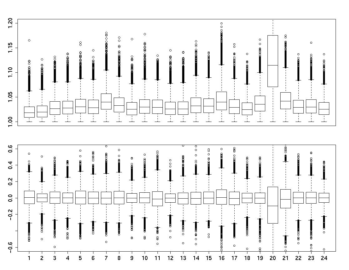
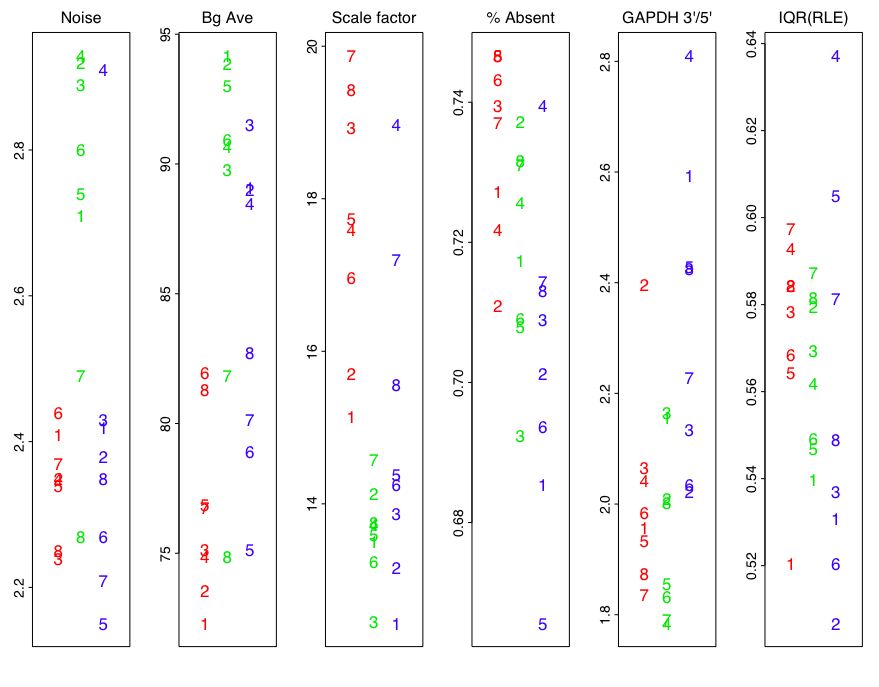
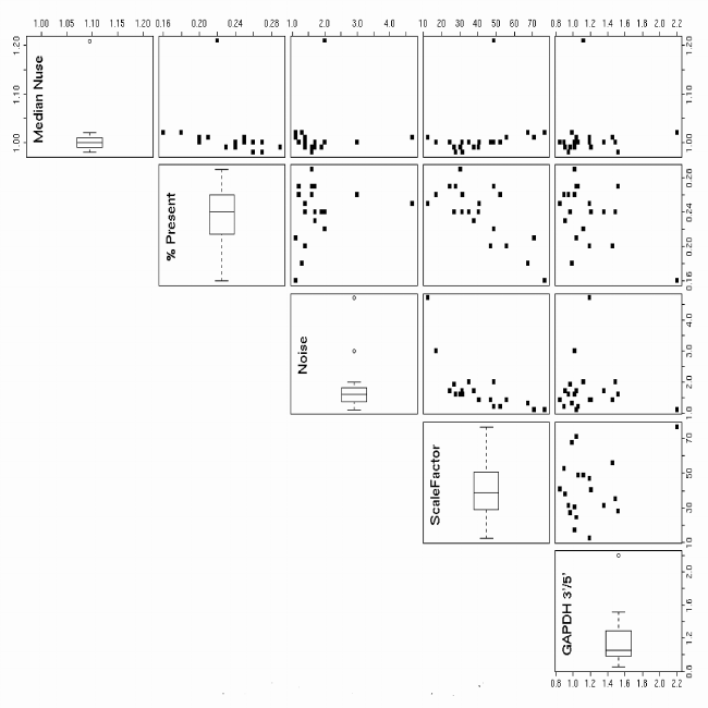
(A) Outlier in the Affymetrix spike-in experiments: 24 HU 95A chips from the Affymetrix spike-in dataset. All but the spike-in probesets are expected to be non-differentially expressed across the arrays. As there are only 14 spike-ins out of about twenty thousand probesets, they are, from the quality assessment point of view, essentially 24 identical hybridizations. A glance at the weight (or residual) landscapes gives a picture of homogenous hybridizations with almost no local defects on any chip but #20 (Fig. A1). The NUSE indicates that chip #20 is an outlier. Its median is well above 1.10, while all others are smaller than 1.05, and its IQR is three and more times bigger than it is for any other chip (Fig. A2). The series of boxplots of the RLE distributions confirms these findings. The median is well below $0,$ and the IQR is two and more times bigger than it is for any other chip. Chip #20 has both a technologically caused bias and a higher noise level. The Affymetrix quality report (Fig. A3), however, does not clearly classify #20 as an outlier. Its GAPDH 3’/5’ of about 2.8 is the largest within this chip set, but the value 2.8 is considered to be acceptable. According to all other Affymetrix quality measures – Percent Present, Noise, Background Average, Scale Factor – chip #20 is within a group of lower quality chips, but does not stand out.

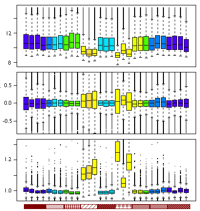
(B) Outlier in St. Jude’s data not detected by the Affymetrix quality report: The collection of MLL HU133B chips consists of 20 chips one of which turns out to be an outlier. The NUSE boxplots (Fig. B1, bottom line) show a median over 1.2 for chip #15 while all others are below 1.025. The IQR is much larger for chip #15 than it is for any other chip. The RLE boxplots (Fig. B1, top line) as well distinguish chip #15 as an obvious outlier. The median is about $-0.2$ for the outlier chip, while it is very close to $0$ for all other chips. The IQR is about twice as big as the largest of the IQR of the other chips. Fig. B1 displays the weight landscapes of chip#15 along with those of two of the typical chips. A region on the left side of chip #15, covering almost a third of the total area, is strongly down weighted, and the chip has elevated weights overall. Affymetrix quality report (Fig. B3) paints a very different picture – Chip $\#$15 is an outlier on the Med(NUSE) scale, but does not stand out on any of common Affymetrix quality assessment measures: Percent Present, Noise, Scale Factor, and GAPDH 3’/5’.

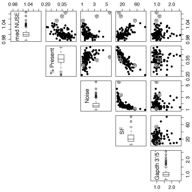
(C) Overall comparison of our measures and the Affymetrix quality report for a large number of St. Jude’s chips: Fig. D1 pairs the Med(NUSE) with the four most common GCOS scores on a set of 129 HU133A chips from the St. Jude dataset. There is noticable linear association between Med(NUSE) and Percent Present, as well as between Med(NUSE) and Scale Factor. GAPDH 3’/5’ does not show a linear association with any the other scores.

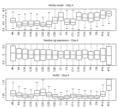
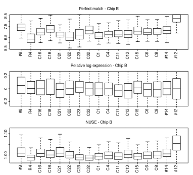
(D) Disagreement between our quality measures and the Affymetrix quality report for Hyperdip$>$50 subgroup in St. Jude’s data: The Affymetrix quality report detects problems with many chips in this dataset. For chip A, Raw Q (Noise) is out of the recommended range for the majority of the chips: $\#$12, $\#$14, C1, C13, C15, C16, C18, C21, C22, C23, C8 and R4. Background detects chip $\#$12 as an outlier. Scale Factor does not show any clear outliers. Percent Present is within the typical range for all chips. GAPDH 3’/5’ is below 3 for all chips. For chip B, Raw Q (Noise) is out of the recommended range for the $\#$12, $\#$8, $\#$18 and R4. Background detects chip $\#$12 and $\#$8 as outliers. Scale Factor does not show any clear outliers. Percent Present never exceeds 23$\%$ in this chip set, and it is below the typical minimum of 20$\%$ for chips $\#$8, C15, C16, C18, C21 and C4. GAPDH 3’/5’ is satisfactory for all chips.

Our measures suggest that, with one exception, the chips are of good quality (Fig. D1). The heterogeneity of the perfect match distributions does not persist after the preprocessing. For chip A, $\#$12 has the largest IQR(RLE) and is a clear outlier among the NUSE distributions. Two other chips have elevated IQR(RLE), but do not stand out according to NUSE. For chip B, the RLE distributions are very similar with $\#$12 again having the largest IQR(RLE). The NUSE distributions are consistently showing good quality with the exception of chip $\#$12.

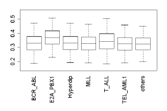
(E) Varying quality between diagnostic subgroups in the St. Jude’s data: Each boxplot in Fig. E1 sketches the Residual Scale Factors (RSF) of the chips of all diagnostic subgroups. They show substantial quality differences. The E2A$\_$PBX1 subgroup has a much higher Med(RSF) than the other subgroups. The T$\_$ALL subgroup has a slightly elevated Med(RSF) and a higher IQR(RSF) than the other subgroups.

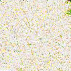
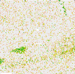
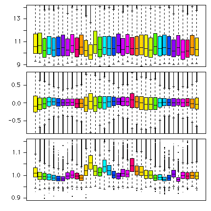
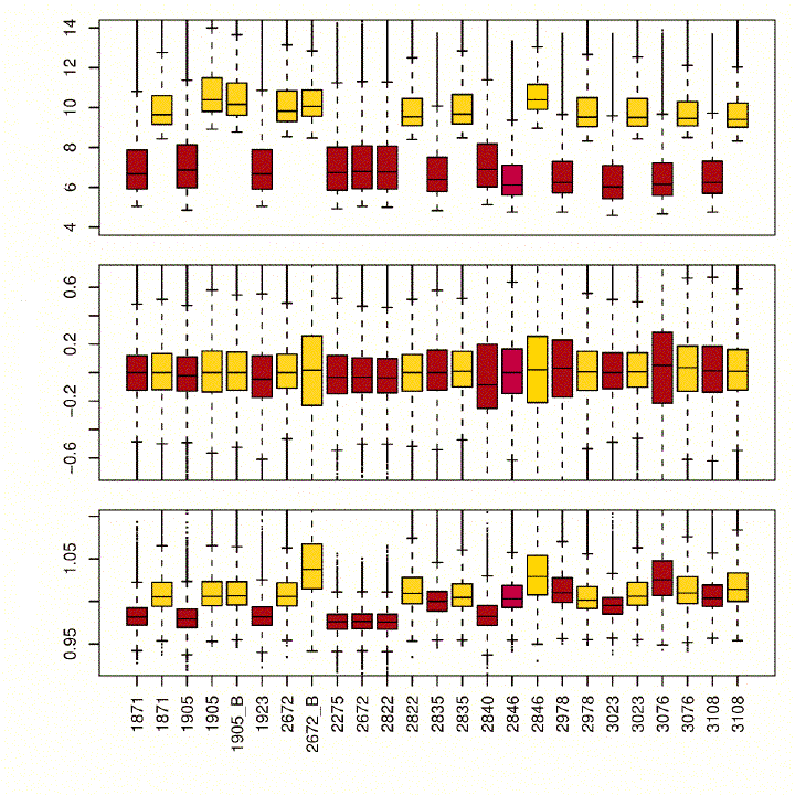
(F) Hybridization date effects on quality of fruit fly chips: The fruit fly mutant with dysfunctional synapses is an experiment of the earlier stages of working with Affymetrix chips in this lab. It shows a wide range of quality. In the boxplot series of RLE and NUSE (Fig. F1) a dependency of the hybridization date is striking. The chips of the two mutants hybridized on the day colored yellow show substantially lower quality than any of the other chips. Fig. F2 shows a weight landscape revealing smooth mountains and valleys. While the pattern is particularly strong in the chip chosen for this picture, it is quite typical for the chips in this dataset. We are not sure about the specific technical reason for this, but assume it is related to insufficient mixing during the hybridization.

(G) Temporal trends or biological variation in fruit fly time series: The series consists of 12 developmental stages of fruit fly embryos hybridized in 3 technical replicates each. While the $log_{2}$(PM) distributions are very similar in all chips, we can spot two kinds of systematic patterns in the RLE and NUSE boxplots (Fig. G1). One pattern is connected to the developmental stage. Within each single one of the three repeat time series, the hybridizations in the middle stages look ”better” than the ones in the early stages and the chips in the late stages. This may, at least to some extent, be due to biological rather than technological variation. In embryo development, especially in the beginning and at the end, huge numbers of genes are expected to be affected, which is a potential violation of assumption (LABEL:M:BioAssumpA). Insufficient staging in the first very short developmental stages may further increase the variability. Also, in the early and late stages of development, there is substantial doubt about the symmetry assumption (LABEL:M:BioAssumpB). Another systematic trend in this dataset is connected to the repeat series. The second dozen chips are of poorer quality than the others. In fact, we learned that they were hybridized on a different day from the rest.

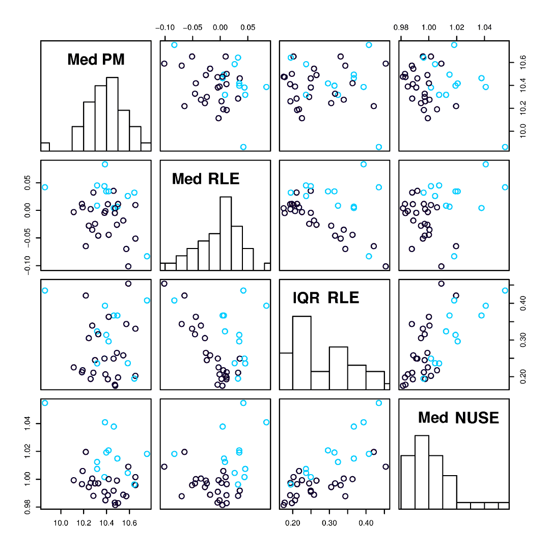
The pairplot in Fig. G2 looks at the relationship between our chip quality measures. There is no linear association between the raw intensities – summarized as Med(PM) – and any of the quality measures. A weak linear association can be noted between Med(RLE) and IQR(RLE). It is worth to note that is becomes much stronger when focusing on just the chips hybridized on the day colored in black. IQR(RLE) and Med(NUSE) again have a weak linear association which becomes stronger when looking only at one of the subgroups, except this time it is the chips colored in gray. For the pairing Med(RLE) and Med(NUSE), however, there is no linear relationship. Finally (not shown), as in the dysfunctional synapses mutant fruit fly dataset, a double-wave gradient, as seen in Fig. F2 for the other fruit fly dataset, can be observed in the quality landscapes of many of the chips. Although these experiments were conducted by a different team of researchers, they used the same equipment as that used in generating the other fruit fly dataset.

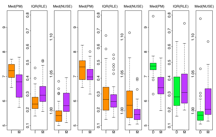
(H) Lab differences in Pritzker’s gender study: We looked at HU95 chip data from 13 individuals in two brain regions, the cortex of the cerebellar hemisphere (short: cerebellum) and the dorsolateral prefrontal cortex. With some exceptions, each sample is hybridized in both lab M and lab I. The NUSE and RLE boxplots (Fig. H1) for the cerebellum dataset display an eye-catching pattern: They show systematically much better quality in Lab M then in Lab I. This might be caused by overexposure or saturation effects in Lab I. The medians of the raw intensities (PM) values in Lab I are, on a $log_{2}$-scale between about 9 and 10.5, while they are very consistently about 2 two 3 points lower in Lab M. The dorsolateral prefrontal cortex hybridizations show, for the most part, a lab effect similar to the one we saw in the cerebellum chips (plots not shown here).

(I) Lab differences in Pritzker’s mood disorder study: After the experiences with lab differences in the gender study, the consortium went through extended efforts to minimize these problems. In particular, the machines were calibrated by Affymetrix specialists. Fig. I1 summarizes the quality assessments of three of the Pritzker mood disorder datasets. We are looking at HU95 chips from two sample cohorts (a total of about 40 subjects) in each of the brain regions anterior cingulate cortex, cerebellum, and dorsolateral prefrontal cortex. In terms of Med(PM), for each of the three brain regions, the two replicates came closer to each other: the difference between the two labs in the mood disorder study is a third or less of the difference between the two labs in the gender study (see first two boxes in each of the three parts of Fig. I1, and compare with Fig. H1). This is due to lab I dropping in intensity (toward lab M) and the new lab D also operating at that level. The consequence of the intensity adjustments for chip quality do not form a coherent story. While for cerebellum the quality in lab M is still better than in the replicate in one of the other labs, for the other two brain regions the ranking is reversed. Effects of a slight underexposure in lab M may now have become more visible. Generally, in all brain regions, the quality differences between the two labs are still there, but they are much smaller than they in the gender study data.

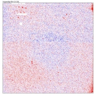
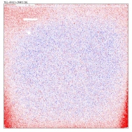
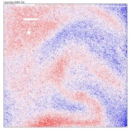
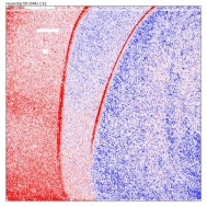
(J) Assigning special causes of poor quality for St. Jude’s data: Eight quality landscapes from the early St. Jude’s data, a collection of 335 HU133Av2 chips. The examples were picked for being particularly strong cases of certain kinds of shortcomings that repeatedly occur in this chip collection. They do not represent the general quality level in the early St. Jude’s chips, and even less so the quality of later St. Jude’s chips. The figures in this paper are in gray levels. If the positive residual landscape is shown, the negative residual landscape is typically some sort of complementary image, and vice versa. Colored quality landscapes for all St. Jude’s chips can be downloaded from Bolstad’s Chip Gallery at www.plmimagegallery.bmbolstad.com.

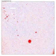
Fig. J1 ”Bubbles” is the positive residual landscape of chip Hyperdip-50-02. There are small dots in the left upper part of the slide, and two bigger ones in the middle of the slide. We attribute the dots to dust attached to the slide or air bubbles stuck in this place during the hybridization. Further, there is an accumulation of positive residuals in the bottom right corner. Areas of elevated residuals near the corners and edges of the slide are very common, often much larger than in this chip. Mostly they are positive. The most likely explanation are air bubbles that, due to insufficient mixing during the hybridization, got stuck close to the edges where they had gotten when this edges was in a higher position to start with or brought up there by the rotation. Note that there typically is some air in the solution injected into the chip (through a little hole near one of the edges), but that the air is moved around by the rotation during the hybridization to minimize the effects on the probe measurements.

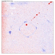
Fig. J2 ”Circle and stick” is the residual landscape of Hyperdip47-50-C17. This demonstrates two kinds of spatial patterns that are probably caused by independent technical shortcomings. First, a circle with equally spaced darker spots (approximately). The symmetry of the shape suggests it was caused by a foreign object scratching trajectories of the rotation during the hybridization into the slide. Second, there are little dots that almost seem to be aligned along a straight line connecting the circle to the upper right corner. The dots might be air bubbles stuck to some invisible thin straight object or scratch.

Fig. J3 ”Sunset” is the negative residual landscape of Hyperdip-50-C6. This chip illustrates two independent technical deficiencies. First, there is a dark disk in the center of the slide. It might be caused by insufficient mixing, but the sharpness with which the disk is separated from the rest of the image asks for additional explanations. Second, the image obviously splits into an upper and a lower rectangular part with different residual, separated by a straight border. As a most likely explanation, we attribute this to scanner problems.

Fig. J4 ”Pond” is the negative residual landscape of TEL-AML1-2M03. The nearly centered disc covers almost the entire slide. It might be caused by the same mechanisms that were responsible for the smaller disc in the previous figure. However, in this data collection, we have only seen two sizes of discs – the small disk as in the previous figure and the large one as in this figure. This raises the question why the mechanism that causes them does not produce medium size discs.

Fig. J5 ”Letter S” is the positive residual landscape of Hypodip-2M03. The striking pattern – the letter ’S’ with the ”cloud” on top – is a particularly curious example of a common technical shortcoming. We attribute the spatially heterogeneous distribution of the residuals to insufficient mixing of the solution during the hybridization.

Fig. J6 ”Compartments” is the positive residual landscape of Hyperdip-50-2M02. This is a unique chip. One explanation would be that the vertical curves separating the three compartments of this image are long thin foreign objects (e.g. hair) that got onto the chip and blocked or inhabited the liquid from being spread equally over the entire chip.

Fig. J7 ”Triangle” is the positive residual landscape of TEL-AML1-06. The triangle might be caused by a long foreign object stuck to the center of the slide on one end and free, and hence manipulated by the rotation, on the other end.

Fig. J8 ”Fingerprint” is the positive residual landscape of Hyperdip-50-C10. What looks like a fingerprint on the picture might actually be one. With the slide measuring 1cm by 1cm, the pattern has about the size of a human fingerprint or the middle part of it.

7 Discussion

Quality landscapes: The pair of the positive and negative residual landscapes contains the maximum information. Often, one of the two residual landscapes can already characterize most of the spatial quality issues. In the weight pictures, the magnitude of the derivation is preserved, but the sign is lost. Therefore, unrelated local defects can appear indistinguishable in weight landscapes. The landscapes allow a first glance at the overall quality of the array: A square filled with low-level noise typically comes from a good quality chip, one filled with high-level noise comes from a chip with uniformly bad probes. If the landscape is reveals any spatial patterns, the quality may or may not be compromised depending on the size of the problematic area. Even a couple of strong local defects may not lower the chip quality, as indicated by our measures. The reason lies in both the chip design and the RMA model. The probes belonging to one probeset are scattered around the chip assuring that a bubble or little scratch would only affect a small number of the probes in a probeset; even a larger under- or overexposed area of the chip may affect only a minority of probes in each probeset. As the RMA model is fitted robustly, its expression summaries are shielded against this kind of disturbance.

We found the quality landscape most useful in assigning special causes of poor chip quality. A quality landscape composed of smooth mountains and valleys is most likely caused by insufficient mixing during the hybridization. Smaller and sharper cut-out areas of elevated residuals are typically related to foreign objects (dust, hair, etc.) or air bubbles. Symmetries can indicate that scratching was caused by particles being rotated during hybridization. Patterns involving horizontal lines may be caused by scanner miscalibration. It has to be noted, that the above assignment of causes are educated guesses rather than facts. They are the result of extensive discussions with experimentalist, but there remains a speculative component to them. Even more hypothetical are some ideas we have regarding how the sign of the residual could reveal more about the special cause. All we can say at this point is that the background corrected and normalized probe intensity deviate from what the fitted RMA model would expect them to be. The focus in this paper is a global one: chip quality. Several authors have worked on spatial chip images from a different perspective, that of automatically detecting and describing local defects (see Reimers and Weinstein (2005), or the R-package Harshlight by Suárez-Fariñas et al. (2005)). It remains an open question how to use this kind of assessment beyond the detection and classification of quality problems. In our approach, if we do not see any indication of quality landscpape features in another quality indicator such as NUSE or RLE, we suppose that it has been rendered harmless by our robust analysis. This may not be true.

RLE: Despite its simplicity the RLE distribution turns out to be a powerful quality tool. For a small number of chips, boxplots of the RLE distributions of each chip allow the detection of outliers and temporal trends. The use of colors or gray levels for different experimental conditions or sample properties facilitates the detection of more complex patterns. For a large number of chips, the IQR(RLE) is a convenient and informative univariate summary. Med(RLE) should be monitored as well to detect bias. As seen in the Drosophila embryo data, these assumptions are crucial to ensuring that what the RLE suggests really are technical artifacts rather than biological differences. Note that the RLE is not tied to the RMA model, but could as well be computed based on expression values derived from other algorithms. The results may differ, but our experience is that the quality message turns out to be similar.

NUSE: As in the case of the RLE, boxplots of NUSE distributions can be used for small chip sets, and plots of their median and interquartile ranges serve as a less space consuming alternative for larger chip sets. For the NUSE, however, we often observe a very high correlation between median and interquartile range, so keeping track of just the median will typically suffice. Again, colors or gray levels can be used to indicate experimental conditions facilitating the detection their potential input on quality. The NUSE is the most sensitive of our quality tools, and it does not have a scale. Observed quality differences, even systematic ones, have therefore to carefully assessed. Even large relative differences do not necessarily compromise an experiment, or render useless batches of chips within an experiment. They should always alert the user to substantial heterogeneity, whose cause needs to be investigated. On this matter we repeat an obvious but important principle we apply. When there is uncertainty about whether or not to include a chip or set of chips in an analysis, we can do both analyses and compare the results. If no great differences result, then sticking with the larger set seems justifiable.

Raw intensities and quality measures: Raw intensities are not useful for quality prediction by itself, but they can provide some explanation for the poor performance according to the other quality measures. All the Pritzker datasets, for example, suffer from systematic differences in the location of the PM intensity distribution (indicated by Med(PM)). Sometimes the lower location was worse – too close to underexposure – and sometimes the higher was worse – too close to overexposure or saturation. We have seen examples of chips for which the raw data give misleading quality assessment. Some kinds of technological shortcomings can be removed without trace by the statististical processing, while others remain.

Comparison with Affymetrix quality scores: We found good overall agreement between our quality assessment and two of the Affymetrix scores: Percent Present and Scale Factor. Provided the quality in a chips set covers a wide enough range, we typically see at least a weak linear association between our quality measures and these two, and sometimes other Affymetrix quality scores. However, our quality assessment does not always agree with the Affymetrix quality report. In the St. Jude data collection we saw that the sensitivity of the Affymetrix quality report could be insufficient. While our quality assessment based on RLE and NUSE clearly detected the outlier chip in the MLL chip B dataset, none of the measures in the Affymetrix quality did. The reverse situation occured in the Hyperdip chip A dataset. While most of the chips passed according to our quality measures, most of the chips got a poor Affymetrix quality scores.

RSF: The Residual Scale Factor can detect quality differences between parts of a data collection, such as the diagnostic subgroups in the St. Jude’s data. In the same way, it can be employed to investigate quality differences between other dataset divisions defined by sample properties, lab site, scanner, hybridization day, or any other experimental condition. More experience as to what magnitudes of differences are acceptable is still needed.

8 Conclusions and Future Work

In this paper, we have laid out a conceptual framework for a statistical approach for the assessment and control of microarray data quality. In particular, we have introduced a quality assessment toolkit for short oligonucleotide arrays. The tools highlight different aspects in the wide spectrum of potential quality problems. Our numerical quality measures, the NUSE and the RLE, are an efficient way to detect chips of unusually poor quality. Furthermore, they permit the detection of temporal trends and patterns, batch effects, and quality biases related to sample properties or to experimental conditions. Our spatial quality methods, the weight and residual landscapes, add to the understanding of specific causes of poor quality by marking those regions on the chip where defects occur. Furthermore, they illustrate the robustness of the RMA algorithm to small local defects. The RSF quantifies quality differences between batches of chips. It provides a broader framework for the quality scores of the individual chips in an experiment. All the quality measures proposed in this paper can be computed based on the raw data using publicly available software.

Deriving the quality assessment directly from the statistical model used to compute the expression values is more powerful than basing it on the performance of a particular set of of control probes, because the control probes may not behave in a way that is representative for the whole set of probes on the array. The model-based approach is also preferable to metrics less directly related to the bulk of the expression values. Some of the Affymetrix metrics, for example, are derived from the raw probe values and interpret any artifacts as quality problems, even if they are removed by routine preprocessing steps. A lesson from the practical examples in this paper is the importance of a well designed experiment. One of the most typical sources for bias, for example, is an unfortunate systematic connection between hybridization date and groups of the study – a link that could have been avoided by better planning.

More research needs to be done on the attribution of specific causes to poor quality measurements. While our quality measures, and, most of all, our quality landscapes, are a rich source for finding specific causes of poor quality, a speculative component remains. To increase the credibility of the diagnoses, systematic quality experiments need to be conducted. A big step forward is Bolstad’s Chip Gallery at www.plmimagegallery.bmbolstad.com, which collects quality landscapes from Affymetrix chip collections, provides details about the experiment and sometimes offers explanations for the technical causes of poor quality. Started as a collection of chip curiosities this website is now growing into a visual encyclopedia for quality assessment. Contributions to the collection, in particular those with known causes of defects, are invited (anonymous if preferred). Further methodological research is needed to explore the use of the spatial quality for statistically ”repairing” local defects, or making partial use of locally damaged chips.

We are well aware that the range of acceptable values for each quality scores is the burning question for experimentalists. Our quality analysis results with microarray datasets from a variety of scientific studies in Section ?? show that the question about the right threshold for good chip quality does not have a simple answer yet, at least not as the present level of generality. Thresholds computed for gene expression measurements in fruit fly mutant screenings can not necessarily be transferred to brain disease research or to leukemia diagnosis. Thresholds need to be calibrated to the tissue type, the design, and the precision needs of the field of application. We offer two strategies to deal with this on different levels:

1. Individual researchers: We encouraged researchers to look for outliers and artificial patterns in the series of quality measures of the batch of jointly analyzed chips. Furthermore, any other form of unusual observations – e.g. a systematic disagreement between NUSE and RLE, or inconsistencies in the association between raw intensities and quality measures – potentially hints at a quality problem in the experiment.

2. Community of microarray users: We recommend the development of quality guidelines. They should be rooted in extended collections of datasets from scientific experiments. Complete raw datasets are ideal, where no prior quality screening has been employed. Careful documentation of the experimental conditions and properties help to link unusual patterns in the quality measures to specific causes. The sharing of unfiltered raw chip data from scientific experiments on the web and the inclusion of chip quality scores in gene expression databank entries can lead the way towards community-wide quality standards. Besides, it contributes to a better understanding how quality measures relate to special causes of poor quality. In addition, we encourage the conduction of designed microarray quality experiments. Such experiments aim at an understanding of the effects of RNA amount, experimental conditions, sample properties and sample handling on the quality measures as well as on the downstream analysis. They give an idea of the range of chip quality to be expected under given certain experimental, and, again, they help to characterize specific causes of poor quality.

Benchmarking of microarray data quality will happen one way or another; if it is not established by community-wide agreements the individual experimentalist will resort to judging on the basis of anecdotal evidence. We recommend that benchmarks be actively developed by the community of microarray researchers, experimentalists and data analysts. The statistical concepts and methods proposed here may serve as a foundation for the quality benchmarking process.

9 Acknowledgement

We thank St. Jude Children’s Research Hospital, the Pritzker Consortium, Tiago Magalhães, Pavel Tomanc̆ák and Affymetrix for sharing their data for quality assessment purposes.

Figures

Figure A1: Weight landscapes of two chips from the Affymetrix HU95 spike-in experiment. The chip on the right-hand side is typical for this data set, only tiny local defects and an overall good probe performance. The chip of the left-hand side (chip $\#$20) has more down-weighted probes all over the slide, and it has a large down-weighted area in the upper left part of the slide

Figure A2: Series of boxplots of NUSE (first row) and RLE (second row) of 24 chips from the Affymetrix HU95 spike-in experiment. Chip $\#$20 is a clear outlier according to all our quality measures: Med(RLE), IQR(RLE), Med(NUSE) and IQR(NUSE)

Figure A3: Affymetrix quality scores and IQR(RLE) for the 24 chips from the Affymetrix HU95 spike-in experiment with the 3 technical replicates in different gray levels (left/center/right in each vertical plot). The outlier chip $\#$20 from Figure A2 is the chip $\#$4 blue in this figure. It is caught by GAPDH 3’/5’. By all other Affymetrix quality measures it is placed within the group of lower quality chips, but it does not stand out

Figure B1: Series of boxplots of RLE (first line) and NUSE (second line) for all 20 MLL 133B chips from St. Jude’s. Chip $\#$15 is an outlier according to all our quality measures: Med(RLE), IQR(RLE), Med(NUSE) and IQR(NUSE)

Figure B2: Weight images for some of St. Jude’s MLL HU133B chips. Chip $\#$10 and chip $\#$11 show low weights overall and small areas with higher weights. Chip $\#$15 has elevated weights overall and a region covering almost a third of the total area with extremly high weights

Figure B3: Med(NUSE) versus GCOS quality report scores for 20 MLL HU133B chips from St. Jude’s data. The outlier chip $\#$15 is in the normal range according to all GCOS quality scores

Figure C1: Med(NUSE) versus GCOS quality report scores for 129 St. Jude’s HU133A chips. Chips with top three Med(NUSE) values are highlighted. Med(NUSE) shows a linear association with Percent Present and with Scale Factor. Noise shows some association with Scale Factor, though not quite a linear one. However, the association between Noise and Med(NUSE) is very weak. GAPDH 3’/5’ does not show a linear association with any of the GCOS scores nor with Med(NUSE)

Figure D1. Boxplots of qualilty measures for St. Jude’s Hyperdip HU133A chips. Perfect match distributions are heterogeneous. $\#$12, $\#$8 and $\#$14 have elevated IQR(RLE). $\#$12 is a clear outlier in NUSE. The bulk of the chips are of good quality according to both NUSE and RLE.

Figure D2. Boxplots of qualilty measures for St. Jude’s Hyperdip HU133B chips. Perfect match distributions are heterogeneous. $\#$12 has elevated IQR(RLE). $\#$12 is a clear outlier in NUSE. The bulk of the chips are of good quality according to both NUSE and RLE.

Figure E1: Boxplots of the estimated residual scales for diagnostic subgroups in the St. Jude’s dataset. They show noticable quality differences

Figure F1: Series of boxplots of log-scaled PM intensities (first row), RLE (second row) and NUSE (third row) for a comparison of nine fruit fly mutants with 3 to 4 technical replicates each. The patterns below the plot indicate mutants and the colors of the boxes indicate hybridization dates. Med(RLE), IQR(RLE), Med(NUSE) and IQR(NUSE) all indicate substantially lower quality on the day colored indigo

Figure F2: “Waves”. Weight image for a typical chip in the fruit fly mutant dataset.
  

Figure G1: Series of boxplots of log-scaled PM intensities (first row), RLE (second row) and NUSE (third row) in the fruit fly development data. Boxes 1-12 represent 12 developmental stages (visualized by different colors), boxes 13-24 and boxes 25-36 represent replicates of the whole series. Replicate series B (boxes 13-24) was hybridized on a different day than the other two series. Both RLE and NUSE indicate lower quality for series B. The first couple of chips and the last couple of chips of each series are different from the rest in terms of Med(RLE) deviating from zero (in varying direction), IQR(RLE) being larger, Med(NUSE) being elevated. This is probably mainly driven by the increased high biological variability in these stages

Figure G2: Paired quality measures for fruit fly development with chips colored depending on the day of the hybridization. Med(PM) has no linear association with any of the other measures. IQR(RLE) and Med(NUSE) show a linear association on the day colored in light blue and a weak linear association on the day colored in black

Figure H1: Series of boxplots of log-scaled PM intensities (first row), RLE (second row) and NUSE (third row) for Pritzker gender study brain samples hybridized in two labs (some replicates missing). Color indicates lab site (dark for lab M, light for lab I). The PM intensity distributions are all located around 6 for lab M, and around 10 for lab I. These systematic lab site differences are reflected by IQR(RLE), Med(NUSE) and RLE(NUSE), which consistently show substantially lower quality for lab hybridizations than for lab M hybridizations

Figure I1: Three brain regions from Pritzker mood disorder dataset, each sample hybridized in two labs (lab site indicated by the letters I, M and D, as well as by colors of the boxes). The boxplots sketch the distribution of quality measure summaries across entire sets of about 40 chips each. There are still differences between the Med(PM) of the two different labs, but they are relatively small. In cerebellum, lab M still produced slightly higher quality hybridizations than lab I, while the ranking is reversed and more pronounced in anterior cingulate cortex. In dorsolateral prefrontal cortex, lab M shows slightly lower quality than the replicate site D

J1. ”Bubbles”

J2. ”Circle and Stick”

J3. ”Sunset”

J4. ”Pond”

J5. ”Letter S”

J6. ”Compartments”

J7. ”Triangle”

J8. ”Fingerprint”

Figure J1-8: Quality landscapes of some selected early St. Jude’s chips

References

- Affymetrix (2001) Affymetrix (2001), Guidelines for assessing data quality, Affymetrix Inc, Santa Clara, CA.
- Alizadeh et al. (2000) Alizadeh, A. A., Eisen, M. B., Davis, R. E., Ma, C., Lossos, I. S., Rosenwald, A., Boldrick, J. C., Sabet, H., Tran, T., Yu, X., Powell, J. I., Yang, L., Marti, G. E., Moore, T., Hudson, J., Lu, L., Lewis, D. B., Tibshirani, R., Sherlock, G., Chan, W. C., Greiner, T. C., Weisenburger, D. D., Armitage, J. O., Warnke, R., Levy, R., Wilson, W., Grever, M. R., Byrd, J. C., Botstein, D., Brown, P. O., and Staudt, L. M. (2000), “Distinct types of diffuse large B-cell lymphoma identified by gene expression profiling,” Nature, 403, 503–511.
- Allison et al. (2006) Allison, D., Cui, X., Page, G., and Sabripour, M. (2006), “Microarray data analysis: from disarray to consolidation and consensus,” Nature Review Genetics, 7, 55–65.
- Archer et al. (2006) Archer, K., Dumur, C., Joel, S., and Ramakrishnan, V. (2006), “Assessing quality of hybridized RNA in Affymetrix GeneChip experiments using mixed effects models,” Biostatistics, 7, 198–212.
- Barczak et al. (2003) Barczak, A., Rodriguez, M., Hanspers, K., Koth, L., Tai, Y., Bolstad, B., Speed, T., and Erle, D. (2003), “Spotted long oligonucleotide arrays for human gene expression analysis,” Genome Research, 1, 1775–1785.
- Beissbarth et al. (2000) Beissbarth, T., Fellenberg, K., Brors, B., Arribas-Prat, R., Boer, J., Hauser, N. C., Scheideler, M., Hoheisel, J. D., Schutz, G., Poustka, A., and Vingron, M. (2000), “Processing and quality control of DNA array hybridization data,” Bioinformatics, 16, 1014–1022.
- Bild et al. (2006) Bild, A., Yao, G., Chang, J., Wang, Q., Potti, A., Chasse, D., Joshi, M., Harpole, D., Lancaster, J., Berchuck, A., Olson, J. J., Marks, J., Dressman, H., West, M., and Nevins, J. (2006), “Oncogenic pathway signatures in human cancers as a guide to targeted therapies,” Nature, 439(7074), 353–357.
- Bolstad (2003) Bolstad, B. (2003), “Low Level Analysis of High-density Oligonucleotide Array Data: Background, Normalization and Summarization,” Ph.D. thesis, University of California, Berkeley, http://bmbolstad.com.
- Bolstad et al. (2005) Bolstad, B., Collin, F., Brettschneider, J., Simpson, K., Cope, L., Irizarry, R., and Speed, T. (2005), “Quality Assessment of Affymetrix GeneChip Data,” in Bioinformatics and Computational Biology Solutions Using R and Bioconductor, eds. Gentleman, R., Carey, V., Huber, W., Irizarry, R., and Dudoit, S., New York: Springer, Statistics for Biology and Health, pp. 33–48.
- Bolstad et al. (2004) Bolstad, B., Collin, F., Simpson, K., Irizarry, R., and Speed, T. (2004), “Experimental design and low-level analysis of microarray data,” Int Rev Neurobiol, 60, 25–58.
- Bolstad et al. (2003) Bolstad, B., Irizarry, R., Astrand, M., and Speed, T. (2003), “A comparison of normalization methods for high density oligonucleotide array data based on variance and bias,” Bioinformatics, 19, 185–193, Evaluation studies.
- Buness et al. (2005) Buness, A., Huber, W., Steiner, K., Sultmann, H., and Poustka, A. (2005), “arrayMagic: two-colour cDNA microarray quality control and preprocessing,” Bioinformatics, 21, 554–556.
- Bunney et al. (2003) Bunney, W., Bunney, B., Vawter, M., Tomita, H., Li, J., Evans, S., Choudary, P., Myers, R., Jones, E., Watson, S., and Akil, H. (2003), “Microarray technology: a review of new strategies to discover candidate vulnerability genes in psychiatric disorders,” Am J Psychiatry, 160, 657–666.
- Cho et al. (1998) Cho, R., Campbell, M., Winzeler, E., Steinmetz, L., Conway, A., Wodicka, L., Wolfsberg, T., Gabrielian, A., Landsman, D., Lockhart, D., and Davis, R. (1998), “A genome-wide transcriptional analysis of the mitotic cell cycle,” Mol Cell, Jul 2(1), 65–73.
- Cui et al. (2005) Cui, X., Hwang, J., Qiu, J., Blades, N., and Churchill, G. (2005), “Improved statistical tests for differential gene expression by shrinking variance components estimates,” Biostatistics, 6, 31–46.
- Dobbin et al. (2005) Dobbin, K., Beer, D., Meyerson, M., Yeatman, T., Gerald, W., Jacobson, W., Conley, B., Buetow, K., Heiskanen, M., Simon, R., Minna, J., Girard, L., Misek, D., Taylor, J., Hanash, S., Naoki, K., Hayes, D., Ladd-Acosta, C., Enkemann, S., Viale, A., and Giordano, T. (2005), “Interlaboratory comparability study of cancer gene expression analysis using oligonucleotide microarrays,” Clin Cancer Res, 11, 565–572.
- Draghici et al. (2006) Draghici, S., Khatri, P., Eklund, A., and Szallasi, Z. (2006), “Reliability and reproducibility issues in DNA microarray measurements,” Trends in Genetics, 22 (2), 101–109.
- Dudoit et al. (2003) Dudoit, S., Shaffer, J., and Boldrick, J. (2003), “Multiple hypothesis testing in microarray experiments,” Statistical Science, 18, 71–103.
- Dudoit et al. (2002) Dudoit, S., Yang, Y., Speed, T., and MJ, C. (2002), “Statistical methods for identifying differentially expressed genes in replicated cDNA microarray experiments,” Statistica Sinica, 12, 111–139.
- Dumur et al. (2004) Dumur, C., Nasim, S., Best, A., Archer, K., Ladd, A., Mas, V., Wilkinson, D., Garrett, C., and Ferreira-Gonzalez, A. (2004), “Evaluation of quality-control criteria for microarray gene expression analysis,” Clin Chem, 50, 1994–2002.
- Efron et al. (2001) Efron, B., Tibshirani, R., Storey, J., and V, T. (2001), “Empirical Bayes analysis of a microarray experiment,” J Am Stat Ass, 96, 1151–1160.
- Finkelstein (2005) Finkelstein, D. (2005), “Trends in the quality of data from 5168 oligonucleotide microarrays from a single facility,” J Biomol Tech, 16, 143–153.
- Finkelstein et al. (2002) Finkelstein, D., Ewing, R., Gollub, J., Sterky, F., Cherry, J., and Somerville, S. (2002), “Microarray data quality analysis: lessons from the AFGC project,” Plant Molecular Biology, 48, 119–131.
- Gassman et al. (1995) Gassman, J., Owen, W., Kuntz, T., Martin, J., and Amoroso, W. (1995), “Data quality assurance, monitoring, and reporting,” Controlled Clinical Trials, 16(2 Suppl), 104S–136S.
- Gautier et al. (2004a) Gautier, L., Cope, L., Bolstad, B., and Irizarry, R. (2004a), “affy - Analysis of Affymetrix GeneChip data at the probe level,” Bioinformatics, 20(3), 307–315.
- Gautier et al. (2004b) Gautier, L., Moller, M., Friis-Hansen, L., and Knudsen, S. (2004b), “Alternative mapping of probes to genes for Affymetrix chips,” BMC Bioinformatics, 5, e111.
- GCOS (2004) GCOS (2004), GeneChip Expression Analysis – Data Analysis Fundamentals, Affymetrix, Inc, Santa Clara, CA.
- Gentleman et al. (2005) Gentleman, R., Carey, V., Huber, W., Irizarry, R., and Dudoit, S. E. (2005), Bioinformatics and Computational Biology Solutions Using R and Bioconductor, Springer.
- Groves (1987) Groves, R. (1987), “Research on survey data quality,” Public Opinion Quaterly, 51, Part 2, Suppl., S156–S172.
- Hautaniemi et al. (2003) Hautaniemi, S., Edgren, H., Vesanen, P., Wolf, M., Järvinen, A., Yli-Harja, O., Astola, J., Kallioniemi, O., and Monni, O. (2003), “A novel strategy for microarray quality control using Bayesian networks,” Bioinformatics, 19, 2031–2038.
- Hoheisel (2006) Hoheisel, J. (2006), “Microarray technology: beyond transcript profiling and genotype analysis,” Nature Review Genetics, 7 (3), 200–210.
- Hu et al. (2005) Hu, P., Greenwood, C., and Beyene, J. (2005), “Integrative analysis of multiple gene expression profiles with quality-adjusted effect size models,” BMC Bioinformatics, 6, e128.
- Hwang et al. (2004) Hwang, K., Kong, S., Greenberg, S., and Park, P. (2004), “Combining gene expression data from different generations of oligonucleotide arrays,” BMC Bioinformatics, 5, e159.
- Irizarry et al. (2003) Irizarry, R., Bolstad, B., Collin, F., Cope, L., Hobbs, B., and Speed, T. (2003), “Summaries of Affymetrix GeneChip probe level data,” Nucleic Acids Res, 31, e15.
- Irizarry et al. (2005) Irizarry, R., Warren, D., Spencer, F., Kim, I., Biswal, S., Frank, B., Gabrielson, E., Garcia, J., Geoghegan, J., Germino, G., Griffin, C., Hilmer, S., Hoffman, E., Jedlicka, A., Kawasaki, E., Martinez-Murillo, F., Morsberger, L., Lee, H., Petersen, D., Quackenbush, J., Scott, A., Wilson, M., Yang, Y., Ye, S., and Yu, W. (2005), “Multiple-laboratory comparison of microarray platforms,” Nat Methods, 2, 345–350.
- Jarvinen et al. (2004) Jarvinen, A.-K., Hautaniemi, S., Edgren, H., Auvinen, P., Saarela, J., Kallioniemi, O.-P., and Monni, O. (2004), “Are data from different gene expression microarray platforms comparable?” Genomics, 83, 1164–1168.
- Jones et al. (2006) Jones, L., Goldstein, D., Hughes, G., Strand, A., Collin, F., Dunnett, S., Kooperberg, C., Aragaki, A., Olson, J., Augood, S., Faull, R., Luthi-Carter, R., Moskvina, V., and Hodges, A. (2006), “Assessment of the relationship between pre-chip and post-chip variables for Affymetrix GeneChip expression data,” BMC Bioinformatics, 7, e211.
- Kerr (2003) Kerr, M. (2003), “Design considerations for efficient and effective microarray studies,” Biometrica, 59, 822–828.
- Kluger et al. (2003) Kluger, Y., Yu, H., Qian, J., and Gerstein, M. (2003), “Relationship between gene co-expression and probe localization on microarray slides,” BMC Genomics, 4, e49.
- Kong et al. (2005) Kong, S., Hwang, K., Kim, R., Zhang, B., Greenberg, S., Kohane, I., and Park, P. (2005), “CrossChip: a system supporting comparative analysis of different generations of Affymetrix arrays,” Bioinformatics, 21, 2116–2117.
- Kuo et al. (2002) Kuo, W., Jenssen, T., Butte, A., Ohno-Machado, L., and Kohane, I. (2002), “Analysis of matched mRNA measurements from two different microarray technologies,” Bioinformatics, 18, 405–412.
- Li and Wong (2001) Li, C. and Wong, H. (2001), “Model-based analysis of oligonucleotide arrays: Expression index computation and outlier detection,” PNAS, 98, 31–36.
- Lipshutz et al. (1999) Lipshutz, R., Fodor, S., Gingeras, T., and Lockhart, D. (1999), “High density synthetic oligonucleotide arrays,” Nat Genet, 21, 20–24.
- Lockhart et al. (1996) Lockhart, D., Dong, H., Byrne, M., Follettie, M., Gallo, M., Chee, M., Mittmann, M., Wang, C., Kobayashi, M., Horton, H., and Brown, E. (1996), “Expression monitoring by hybridization to high-density oligonucleotide arrays,” Nat Biotechnol, 14, 1675–1680.
- Loebl (1990) Loebl, A. (1990), “Accuracy and Relevance and the Quality of Data,” in Data Quality Control, Theory and Pragmatics, eds. Liepins, G. and Uppuluri, V., New York: Marcel Dekker, Inc., no. 112 in Statistics: Textbooks and Monographs, pp. 105–144.
- Lönnstedt and Speed (2002) Lönnstedt, I. and Speed, T. (2002), “Replicated microarray data,” Statistica Sinica, 12 (1), 31–46.
- Marinez et al. (1984) Marinez, Y., McMahan, C., Barnwell, G., and Wigodsky, H. (1984), “Ensuring data quality in medical research through an integrated data management system,” Stat Med, 3, 101–111.
- Mason and Young (2002) Mason, R. and Young, J. (2002), Multivariate statistical process control with industrial applications, Philadelphia, Pennsylvania: ASA-SIAM.
- McLachlan et al. (2004) McLachlan, G., Do, K., and Ambroise, C. (2004), Analyzing Microarray Gene Expression Data, Hoboken, New Jersey: Wiley.
- Mecham et al. (2004) Mecham, B., Klus, G., Strovel, J., Augustus, M., Byrne, D., Bozso, P., Wetmore, D., Mariani, T., Kohane, I., and Szallasi, Z. (2004), “Sequence-matched probes produce increased cross-platform consistency and more reproducible biological results in microarray-based gene expression measurements,” Nucleic Acids Res, 32, 74.
- Mehta et al. (2004) Mehta, T., Tanik, M., and Allison, D. (2004), “Towards sound epistemological foundations of statistical methods for high-dimensional biology,” Nature Genetics, 36, 943–947.
- Mitchell et al. (2004) Mitchell, S., Brown, K., Henry, M., Mintz, M., Catchpoole, D., LaFleur, B., and Stephan, D. (2004), “Inter-platform comparability of microarrays in acute lymphoblastic leukemia,” BMC Genomics, 5, e71.
- Model et al. (2002) Model, F., König, T., Piepenbrock, C., and Adorjan, P. (2002), “Statistical process control for large scale microarray experiments,” Bioinformatics, 18 Suppl 1, 155–163, Evaluation studies.
- Morris et al. (2004) Morris, J., Yin, G., Baggerly, K., Wu, C., and Zhang, L. (2004), “Pooling information across different studies and oligonucleotide microarray chip types to identify prognostic genes for lung cancer,” in Methods of Microarray Data Analysis III, eds. Shoemaker, J. and Lin, S., New York: Springer, pp. 51–66.
- Naef et al. (2003) Naef, F., Socci, N., and Magnasco, M. (2003), “A study of accuracy and precision in oligonucleotide arrays: extracting more signal at large concentrations,” Bioinformatics, 19, 178–184.
- Nimgaonkar et al. (2003) Nimgaonkar, A., Sanoudou, D., Butte, A., Haslett, J., Kunkel, L., Beggs, A., and Kohane, I. (2003), “Reproducibility of gene expression across generations of Affymetrix microarrays,” BMC Bioinformatics, 4, e27.
- Novikov and Barillot (2005) Novikov, E. and Barillot, E. (2005), “An algorithm for automatic evaluation of the spot quality in two-color DNA microarray experiments,” BMC Bioinformatics, 6, e293.
- Perou et al. (2000) Perou, C., Sorlie, T., Eisen, M., van de Rijn, M., Jeffrey, S., Rees, C., Pollack, J., Ross, D., Johnsen, H., Akslen, L., Fluge, O., Pergamenschikov, A., Williams, C., Zhu, S., Lonning, P., Borresen-Dale, A., Brown, P., and Botstein, D. (2000), “Molecular portraits of human breast tumours,” Nature, 406, 747–752.
- Qian et al. (2003) Qian, J., Kluger, Y., Yu, H., and Gerstein, M. (2003), “Identification and correction of spurious spatial correlations in microarray data,” Biotechniques, 35, 42–44, Evaluation studies.
- Ramaswamy and Golub (2002) Ramaswamy, S. and Golub, T. (2002), “DNA microarrays in clinical oncology,” J. Clin. Oncol., 20, 1932–1941.
- Redman (1992) Redman, T. (1992), Data quality: management and technology, New York: Bantam Books.
- Reimers and Weinstein (2005) Reimers, M. and Weinstein, J. (2005), “Quality assessment of microarrays: Visualization of spatial artifacts and quantitation of regional biases,” BMC Bioinformatics, 6, e166.
- Ritchie et al. (2006) Ritchie, M., Diyagama, D., Neilson, J., van Laar, R., A, D., A, H., and GK, S. (2006), “Empirical array quality weights in the analysis of microarray data,” BMC Bioinformatics, 7, e261.
- Rogojina et al. (2003) Rogojina, A., Orr, W., Song, B., and Geisert, E. J. (2003), “Comparing the use of Affymetrix to spotted oligonucleotide microarrays using two retinal pigment epithelium cell lines,” Mol Vis, 9, 482–496.
- Ross et al. (2003) Ross, M., Zhou, X., Song, G., Shurtleff, S., Girtman, K., Williams, W., Liu, H., Mahfouz, R., Raimondi, S., Lenny, N., Patel, A., and Downing, J. (2003), “Classification of pediatric acute lymphoblastic leukemia by gene expression profiling,” Blood, 102, 2951–2959.
- Schoor et al. (2003) Schoor, O., Weinschenk, T., Hennenlotter, J., Corvin, S., Stenzl, A., Rammensee, H., and Stevanovic, S. (2003), “Moderate degradation does not preclude microarray analysis of small amounts of RNA,” Biotechniques, 35, 1192–1196.
- Shewhart (1939) Shewhart, W. (1939), Statistical Method from the Viewpoint of Quality Control, Lanceser, Pennsylvania: Lancester Press, Inc.
- Shippy et al. (2004) Shippy, R., Sendera, T., Lockner, R., Palaniappan, C., Kaysser-Kranich, T., Watts, G., and J, A. (2004), “Performance evaluation of commercial short-oligonucleotide microarrays and the impact of noise in making cross-platform correlations,” BMC Genomics, 5, e61.
- Smith and Hallett (2004) Smith, K. and Hallett, M. (2004), “Towards quality control for DNA microarrays,” J Comput Biol, 11, 945–970.
- Smyth (2002) Smyth, G. (2002), “Print-order normalization of cDNA microarrays,” Tech. rep., Genetics and Bioinformatics, Walter and Eliza Hall Institute of Medical Research, Melbourne, available at www.statsci.org/smyth/pubs/porder/porder.html.
- Smyth et al. (2003) Smyth, G., Yang, H., and Speed, T. (2003), “Statistical Issues in cDNA Microarray Data Analysis,” in Functional Genomics, Methods and Protocols, eds. Brownstein, M. J. and Khodursky, A. B., Totowa, New Jersey: Humana Press, no. 224 in Methods in Molecular Biology, pp. 111–136.
- Speed (2003) Speed, T. (2003), Statistical analysis of gene expression of gene expression microarray data, Boca Raton, Florida: Chapman and Hall/CRC.
- Stevens and Doerge (2005) Stevens, J. and Doerge, R. (2005), “Combining Affymetrix microarray results,” BMC Bioinformatics, 6, e57.
- Storey (2003) Storey, J. (2003), “The positive false discovery rate: A Bayesian interpretation and the q-value,” Annals of Statistics, 31, 2013–2035.
- Suárez-Fariñas et al. (2005) Suárez-Fariñas, M., Haider, A., and Wittkowski, K. (2005), “”Harshlighting” small blemishes on microarrays,” BMC Bioinformatics, 6, e65.
- Subramanian et al. (2005) Subramanian, A., Tamayo, P., Mootha, V., Mukherjee, S., Ebert, B., Gillette, M., Paulovich, A., Pomeroy, S., Golub, T., Lander, E., and Mesirov, J. (2005), “Gene set enrichment analysis: a knowledge-based approach for Interpreting genomewide expression profiles,” PNAS, 102, 155545–50.
- Tai and Speed (2006) Tai, Y. and Speed, T. (2006), “A multivariate empirical Bayes statstic for replicated microarray time course data,” Ann Statist, 34, 2387–2412.
- Thach et al. (2003) Thach, D., Lin, B., Walter, E., Kruzelock, R., Rowley, R., Tibbetts, C., and Stenger, D. (2003), “Assessment of two methods for handling blood in collection tubes with RNA stabilizing agent for surveillance of gene expression profiles with high density microarrays,” J Immunol Methods, 283, 269–279.
- The Chipping Forecast (1999) The Chipping Forecast (1999), The Chipping Forecast I, vol. 21-1s, Nature Genetics Suppl.
- The Chipping Forecast (2002) — (2002), The Chipping Forecast II, vol. 32-4s, Nature Genetics Suppl.
- The Chipping Forecast (2005) — (2005), The Chipping Forecast III, vol. 37-6s, Nature Genetics Suppl.
- Thompson et al. (2005) Thompson, K., Rosenzweig, B., Pine, P., Retief, J., Turpaz, Y., Afshari, C., Hamadeh, H., Damore, M., Boedigheimer, M., Blomme, E., Ciurlionis, R., Waring, J., Fuscoe, J., Paules, R., Tucker, C., Fare, T., Coffey, E., He, Y., Collins, P., Jarnagin, K., Fujimoto, S., Ganter, B., Kiser, G., Kaysser-Kranich, T., Sina, J., and Sistare, F. (2005), “Use of a mixed tissue RNA design for performance assessments on multiple microarray formats,” Nucleic Acid Research, 33 (2), e187.
- Tom et al. (2005) Tom, B., Gilks, W., Brooke-Powell, E., and Ajioka, J. (2005), “Quality determination and the repair of poor quality spots in array experiments,” BMC Bioinformatics, 6, e234.
- Tomanc̆ák et al. (2002) Tomanc̆ák, P., Beaton, A., Weiszmann, R., Kwan, E., Shu, S., Lewis, S., Richards, S., Ashburner, M., Hartenstein, V., Celniker, S., and Rubin, G. (2002), “Systematic determination of patterns of gene expression during Drosophila embryogenesis,” Genome Biol, 3, 1–14.
- Vawter et al. (2004) Vawter, M., Evans, S., Choudary, P., Tomita, H., Meador-Woodruff, J., Molnar, M., Li, J., Lopez, J., Myers, R., Cox, D., Watson, S., Akil, H., Jones, E., and Bunney, W. (2004), “Gender-specific gene expression in post-mortem human brain: localization to sex chromosomes,” Neuropsychopharmacology, 29, 373–384.
- Wang et al. (2005) Wang, H., He, X., Band, M., and Wilson, Cand Liu, L. (2005), “A study of inter-lab and inter-platform agreement of DNA microarray data,” BMC Genomics, 6, e71.
- Wang (2001) Wang, R. (2001), Data quality, Boston: Kluwer Academic Publishers.
- Wang et al. (1995) Wang, R., Storey, V., and Firth, C. (1995), “A framework for analysis of data quality research,” IEEE Transactions of Knowledge and Data Engineering, 7, 623–640.
- Wang et al. (2001) Wang, X., Ghosh, S., and Guo, S. (2001), “Quantitative quality control in microarray image processing and data acquisition,” Nucleic Acids Res, 29 (15), e75.
- Wilson and Miller (2005) Wilson, C. and Miller, C. (2005), “Simpleaffy: a BioConductor package for Affymetrix quality control and data analysis,” Bioinformatics, 21, 3683–3685.
- Wit and McClure (2004) Wit, E. and McClure, J. (2004), Statistics for microarrays: design, analysis, inference, Hoboken, New Jersey: Wiley.
- Woo et al. (2004) Woo, Y., Affourtit, J., Daigle, S., Viale, A., Johnson, K., Naggert, J., and Churchill, G. (2004), “A comparison of cDNA, oligonucleotide, and Affymetrix GeneChip gene expression microarray platforms,” J Biomol Tech, 15, 276–284.
- Yang et al. (2001) Yang, Y., Buckley, M., and Speed, T. (2001), “Analysis of cDNA microarray images,” Brief Bioinform, 2, 341–349.
- Yang et al. (2002) Yang, Y., Dudoit, S., Luu, P., Lin, D., Peng, V., Ngai, J., and Speed, T. (2002), “Normalization for cDNA microarray data: a robust composite method addressing single and multiple slide systematic variation,” Nucleic Acids Res, 30, e15.
- Yauk et al. (2004) Yauk, C., Berndt, M., Williams, A., and Douglas, G. (2004), “Comprehensive comparison of six microarray technologies,” Nucleic Acid Research, 32 (15), e124.
- Yeoh et al. (2002) Yeoh, E., Ross, M., Shurtleff, S., Williams, W., Patel, D., Mahfouz, R., Behm, F., Raimondi, S., Relling, M., Patel, A., Cheng, C., Campana, D., Wilkins, D., Zhou, X., Li, J., Liu, H., Pui, C., Evans, W., Naeve, C., Wong, L., and Downing, J. (2002), “Classification, subtype discovery, and prediction of outcome in pediatric acute lymphoblastic leukemia by gene expression profiling,” Cancer Cell, 1, 133–143.
- Yuen et al. (2002) Yuen, T., Wurmbach, E., Pfeffer, R., Ebersole, B., and Sealfon, S. (2002), “Accuracy and calibration of commercial oligonucleotide and custom cDNA microarrays,” Nucleic Acids Res, 30, e48.
- Zhang et al. (2004) Zhang, W., Shmulevich, I., and Astola, J. (2004), Microarray Quality Control, Hoboken, New Jersey: John Wiley & Sons, Inc.
- Zhu et al. (2005) Zhu, B., Ping, G., Shinohara, Y., Zhang, Y., and Baba, Y. (2005), “Comparison of gene expression measurements from cDNA and 60-mer oligonucleotide microarrays,” Genomics, 85, 657–665.