Relaxational dynamics in 3D randomly diluted Ising models

Abstract

We study the purely relaxational dynamics (model A) at criticality in three-dimensional disordered Ising systems whose static critical behaviour belongs to the randomly diluted Ising universality class. We consider the site-diluted and bond-diluted Ising models, and the $\pm J$ Ising model along the paramagnetic-ferromagnetic transition line. We perform Monte Carlo simulations at the critical point using the Metropolis algorithm and study the dynamic behaviour in equilibrium at various values of the disorder parameter. The results provide a robust evidence of the existence of a unique model-A dynamic universality class which describes the relaxational critical dynamics in all considered models. In particular, the analysis of the size-dependence of suitably defined autocorrelation times at the critical point provides the estimate $z=2.35(2)$ for the universal dynamic critical exponent. We also study the off-equilibrium relaxational dynamics following a quench from $T=\infty$ to $T=T_{c}$. In agreement with the field-theory scenario, the analysis of the off-equilibrium dynamic critical behavior gives an estimate of $z$ that is perfectly consistent with the equilibrium estimate $z=2.35(2)$.

1 Introduction

Randomly diluted uniaxial antiferromagnets, for instance, Fe_pZn_1-pF₂ and Mn_pZn_1-pF₂,   have been much investigated experimentally and theoretically [1, 2, 3, 4]. For sufficiently low impurity concentration $1-p$, these systems undergo a second-order phase transition at $T_{c}(p)<T_{c}(p=1)$. The critical behaviour is approximately independent of the impurity concentration and definitely different from the one of the pure system. These results have been successfully explained by the field-theoretical (FT) renormalisation group (RG), which predicts the presence of a single universality class associated with the paramagnetic-ferromagnetic transition that occurs in Ising systems with quenched random dilution. Monte Carlo (MC) results have been contradictory for a long time, finding model-dependent critical exponents. In [5] this apparent non-universality was shown to be an effect of strong scaling corrections. They are slowly decaying due to the fact that the leading correction-to-scaling exponent $\omega$ is quite small: $\omega=0.29(2)$ (see A).

The analyses significantly gain accuracy when using improved Hamiltonians, for which the leading scaling corrections are suppressed for any thermodynamic quantity, and improved estimators, which are such that the leading scaling correction is suppressed for any model in the same universality class. MC simulations of different improved Hamiltonians [6, 7] confirmed that the static critical behaviour is model-independent, in agreement with the FT description, and provided accurate estimates of the static critical exponents, $\nu=0.683(2)$ and $\eta=0.036(1)$ [6, 8, 5]. They are in good agreement with the FT perturbative results [9] $\nu=0.678(10)$ and $\eta=0.030(3)$ obtained by the analysis of high-order (six-loop) perturbative expansions (similar results are obtained at five loops [10]). The apparent non-universality observed in previous numerical works was mainly due to the fact that scaling corrections were neglected. As a consequence, previous studies did not really observe the asymptotic critical behaviour and only determined effective exponents depending on all parameters of the investigated model.

In this paper we extend the analysis to the critical dynamics. We consider a purely relaxational dynamics without conserved order parameters, also known as model A [11], as appropriate for uniaxial magnetic materials. Experimental results are reported in [12, 13, 14]. According to the FT RG (see, e.g., [15, 16, 17]), the dynamic behaviour should be the same in all RDIs systems, as is the case for the static criticality. Moreover, the leading scaling corrections appearing in dynamical quantities should be associated with the same RG operators that control the nonasymptotic behaviour of static quantities and thus, they should be characterized by the same exponents as in the static case, i.e., by $\omega=0.29(2)$ and $\omega_{2}=0.82(8)$. As a consequence, in the case of improved Hamiltonians, leading scaling corrections should also be absent in dynamical quantities. Therefore, the most precise estimates of dynamic universal quantities should be obtained in improved models, as in the static case.

Previous MC studies [18, 19, 20, 21, 22, 23] of equilibrium and off-equilibrium dynamics apparently have not confirmed the FT general predictions. They have mainly focused on the dynamic critical exponent $z$, which characterizes the divergence of the autocorrelation times when approaching the critical point. In most of the cases they have found that $z$ is model dependent and have provided estimates which range from $z\approx 2.1$ to $z\approx 2.6$, depending apparently on the method, the favoured values of the dilution parameter $p$, whether it is determined from equilibrium or off-equilibrium simulations, etc. In [20, 22] the universality of $z$ was verified, obtaining $z\approx 2.6$, but the leading scaling-correction exponent was not consistent with the static one, as predicted by the FT approach. Moreover, this result is inconsistent with the perturbative FT estimate obtained from analyses of the perturbative expansions [24, 25, 26, 15, 27, 28, 29] at two and three loops, which suggest $z\approx 2.18$.

In this paper we study three disordered Ising systems whose static critical behaviour belongs to the 3D RDIs universality class: the randomly site-diluted Ising model (RSIM), the randomly bond-diluted Ising model (RBIM), and the $\pm J$ Ising model along the paramagnetic-ferromagnetic transition line. Their static critical behaviour was carefully investigated in [6, 7]. In particular, the value $p^{*}$ of the dilution parameter corresponding to an improved model was determined for each of them. We simulate these models by using the Metropolis algorithm (with a suitable modification in the case of the RSIM and RBIM to avoid ergodicity problems, see B), which does not satisfy any conservation law, and thus allows us to investigate the model-A dynamics. We consider cubic lattices of size $L^{3}$ with $8\leq L\leq 64$.

The main purpose is to check whether the dynamic critical behaviour is consistent with the FT RG, that is with the existence of a unique model-A universality class for RDIs systems. We focus on the dynamic critical exponent $z$, and determine it in the RSIM, the RBIM, and the $\pm J$ Ising model. We find that the autocorrelation times extracted from the autocorrelation function of the magnetic suspectibility at $T_{c}$ behave as

$$\tau=cL^{z}(1+c_{11}L^{-\omega}+c_{12}L^{-2\omega}+\cdots+c_{21}L^{-\omega_{2}}+\cdots)$$ (1)

with a universal value of the dynamic exponent $z$. Moreover, $\omega$ and $\omega_{2}$ are consistent with the static scaling-correction exponents $\omega=0.29(2)$ and $\omega_{2}=0.82(8)$. We obtain the estimates $z=2.355(16)$, $z=2.335(18)$, and $z=2.345(17)$, respectively for the RSIM, the RBIM, and the $\pm J$ Ising model at $p\approx p^{*}$. They are in good agreement, strongly supporting universality. Results for other values of $p$, both larger and smaller than $p^{*}$, are consistent with the estimates of $z$ obtained at $p\approx p^{*}$. We consider

$$z=2.35(2)$$ (2)

as our best estimate of $z$ for the dynamic model-A universality class of RDIs systems. These results confirm the general picture that comes out of the FT analysis. However, from a quantitative point of view, our estimate significantly differs from the perturbative result $z\approx 2.18$ at three loops [28, 29]. Apparently, perturbative FT expansions at this order are not able to predict accurately the exponent $z$.

The exponent $z$ can also be determined by performing off-equilibrium simulations, since the approach to equilibrium is controlled by the same FT model [30, 31, 16]. As a further check of our result (2), we have performed off-equilibrium MC simulations of the RSIM at $p=0.8$, quenching $T=\infty$ configurations to $T=T_{c}$. The results show that the relaxation to equilibrium is controlled by the same dynamic exponent obtained in equilibrium simulations, i.e. $z=2.35(2)$. Moreover, the large-time corrections are consistent with what is predicted by the FT RG, which relates them to the static leading and next-to-leading scaling-correction exponents $\omega=0.29(2)$ and $\omega_{2}=0.82(8)$. Our results therefore confirm the FT analysis of the off-equilibrium relaxational dynamics [30, 31, 16].

The paper is organized as follows. In Sec. 2 we define the disordered Ising models that are considered in the paper. In Sec. 3 we define the quantities that are measured in the MC simulation and discuss the FT predictions. In Sec. 4 we report the finite-size scaling (FSS) analysis of equilibrium MC simulations of the RSIM, the RBIM, and the $\pm J$ Ising model. In Sec. 5 we study the off-equilibrium relaxational critical behaviour of the RSIM, in a quench from $T=\infty$ to $T_{c}$. Finally, we draw our conclusions in Sec. 6. In A we refine the estimate of the leading scaling correction exponent, obtaining $\omega=0.29(2)$. Some details on the MC algorithm are discussed in B.

2 Models

We consider the randomly site-diluted Ising model (RSIM) with Hamiltonian

$${\cal H}_{\rho}=-\sum_{<xy>}\rho_{x}\,\rho_{y}\;\sigma_{x}\sigma_{y},$$ (3)

where the sum is extended over all nearest-neighbour sites of a simple cubic lattice, $\sigma_{x}$ are Ising spin variables, and $\rho_{x}$ are uncorrelated quenched random variables, which are equal to 1 with probability $p$ (the spin concentration) and 0 with probability $1-p$ (the impurity concentration). We also consider the randomly bond-diluted Ising model (RBIM) in which the disorder variables are associated with links rather than with sites. It is defined by the Hamiltonian

$${\cal H}_{j}=-\sum_{<xy>}j_{xy}\;\sigma_{x}\sigma_{y},$$ (4)

where the couplings $j_{xy}$ are uncorrelated quenched random variables, which take values 0,1 with probability distribution

$$P(j_{xy})=p\delta(j_{xy}-1)+(1-p)\delta(j_{xy}).$$ (5)

Note that the exchange interaction is ferromagnetic in both models.

MC simulations [6, 7] have provided strong numerical evidence that the static critical behaviour of the RSIM (for $1>p>p_{s}$, where $p_{s}$ is the site-percolation point, $p_{s}=0.3116081(13)$ on a simple cubic lattice [32]) and of the RBIM (for $1>p>p_{b}$, where $p_{b}$ is the bond-percolation point, $p_{b}=0.2488126(5)$ on a simple cubic lattice [33]) belong to the same universality class. The most precise estimates of the static critical exponents have been obtained by MC simulations: [6, 8, 5] $\nu=0.683(2)$ and $\eta=0.036(1)$. These estimates are in good agreement with the perturbative FT results [9, 10] $\nu=0.678(10)$ and $\eta=0.030(3)$, and with experiments [1, 2]. Also the leading and next-to-leading correction-to-scaling exponents have been computed. Here we shall obtain a precise estimate of the leading exponent $\omega$, $\omega=0.29(2)$, by a combined analysis of the data obtained in [6] and those obtained in the present work; see A for details. As for the next-to-leading exponent, we quote the FT estimate obtained in [6], $\omega_{2}=0.82(8)$.

We also consider the $\pm J$ Ising model, defined by Hamiltonian (4) with exchange interactions $j_{xy}$ which take values $\pm 1$ with probability distribution [34]

$$P(j_{xy})=p\delta(j_{xy}-1)+(1-p)\delta(j_{xy}+1).$$ (6)

Unlike the RSIM and the RBIM, the $\pm J$ Ising model is frustrated for any $p$. Nonetheless, the paramagnetic-ferromagnetic transition line that occurs in this model for $0<p<1-p_{N}$ and $p_{N}<p<1$ also belongs to the RDIs universality class [7]. Here $p_{N}$ is the location of the magnetic-glassy Nishimori multicritical point, which has been recently computed in [35]: $p_{N}=0.76820(4)$.

In this work we consider a relaxational dynamics without conserved order parameters, i.e. the so-called model A. In lattice systems this dynamics is usually realized by using the Metropolis algorithm. In the case of the RSIM and of the RBIM however, if a sequential updating scheme is used, the Metropolis algorithm with the standard acceptance probability $P_{A}=$min$[1,\exp(-\beta\Delta{\cal H})]$ is not ergodic and thus it does not provide the correct dynamics. An ergodic dynamics is obtained by introducing a simple modification which is described in B. In the $\pm J$ Ising model we use the standard Metropolis algorithm with a sequential updating scheme. In this model the specific problem we observed in the RSIM and in the RBIM is not present (note, however, that, to our knowledge, a rigorous proof of ergodicity is lacking for this updating scheme; this is also the case of the pure Ising model).

Note that the algorithm with sequential updating does not satisfy detailed balance and hence does not strictly correspond to a reversible dynamics. Detailed balance is satisfied only if the spins are updated in random order. It is commonly accepted that these two dynamics belong to the same universality class: these violations of detailed balance are irrelevant in the critical limit.

3 Autocorrelation times: definitions and critical properties

We consider the two-point correlation function

$$G(x_{2}-x_{1},t_{2}-t_{1})\equiv\overline{\langle\sigma(x_{1},t_{1})\,\sigma(x_{2},t_{2})\rangle},$$ (7)

where the overline indicates the quenched average over the disorder probability distribution and $\langle\cdot\cdot\cdot\rangle$ indicates the thermal average. Near the critical point correlations develop both in space and time. They can be characterized in terms of the equal-time second-moment correlation length $\xi$ and of an autocorrelation time $\tau$. In the infinite-volume limit the correlation length $\xi$ can be defined as

$$\xi^{2}\equiv-{1\over\chi}\left.{\partial\widetilde{G}(k,0)\over\partial k^{2}}\right|_{k^{2}=0},$$ (8)

where $\widetilde{G}(k,t)$ is the Fourier transform of $G(x,t)$ with respect to the $x$ variable and

$$\chi\equiv\sum_{x}G(x,0)=\widetilde{G}(0,0)$$ (9)

is the static magnetic susceptibility. On a finite lattice with periodic boundary conditions, we define $\xi$ as

$$\xi^{2}\equiv{\widetilde{G}(0,0)-\widetilde{G}(q_{\rm min},0)\over\hat{q}_{\rm min}^{2}\widetilde{G}(q_{\rm min},0)},$$ (10)

where $q_{\rm min}\equiv(2\pi/L,0,0)$, $\hat{q}\equiv 2\sin q/2$. To define the autocorrelation time, we consider the autocorrelation function $A(t)$ of a long-distance quantity. Then, we define the integrated autocorrelation time

$$\tau_{{\rm int}}\equiv{1\over 2}\sum_{t=-\infty}^{\infty}\,{A(t)\over A(0)}={1\over 2}+\sum_{t=1}^{\infty}\,{A(t)\over A(0)}.$$ (11)

Here $t$ is the Metropolis time and one time unit corresponds to a complete lattice sweep.

In the critical limit $\xi$ and the autocorrelation time $\tau_{{\rm int}}$ diverge. If $t_{r}\equiv(T-T_{c})/T_{c}$ and $T_{c}$ is the critical temperature, for $|t_{r}|\to 0$ we have in the thermodynamic limit

$$\xi\sim|t_{r}|^{-\nu},\qquad\tau_{{\rm int}}\sim|t_{r}|^{-z\nu}\sim\xi^{z},$$ (12)

where $\nu$ is the usual static exponent and $z$ is a dynamic exponent that depends on the considered dynamics.

The correlation function $\widetilde{G}(k,t)$ is the quantity of direct experimental interest and thus we could take $A(t)=\widetilde{G}(k,t)$. However, for the determination of the dynamic critical exponent $z$, it is computationally more convenient to use a different quantity. We consider the autocorrelation function of the magnetic susceptibility

$$A(t)=\overline{\langle S(0)S(t)\rangle-\langle S\rangle^{2}},\qquad S(t)\equiv{1\over V}\Bigl{[}\sum_{x}\sigma(x,t)\Bigr{]}^{2}.$$ (13)

Using (11) we could determine the autocorrelation time $\tau_{{\rm int}}$ and then, we could use it to determine $z$. However, the determination of this quantity requires the knowledge of the large-$t$ behaviour of $A(t)$. Since it is difficult to determine it precisely, $\tau_{{\rm int}}$ is unsuitable for a high-precision study. We now introduce a new time scale which is particularly convenient numerically. Let us define

$$\tau_{\rm eff}(t+n/2)\equiv{n\over\ln[A(t)/A(t+n)]},$$ (14)

where $n$ is a fixed integer number. A linear interpolation can be used to extend $\tau_{\rm eff}(t)$ to all real numbers. Then, for any positive $x$, we define an autocorrelation time $\tau_{x}$ as the solution of the equation

$$\tau_{x}=\tau_{\rm eff}(x\tau_{x}).$$ (15)

This definition is based on the idea that, if $A(t)$ were a pure exponential, i.e., $A(t)=A_{0}\exp(-t/\tau)$, then $\tau_{\rm eff}(t)=\tau$ for all $t$ and thus $\tau_{x}=\tau$ for any $x$.

Let us now consider the thermodynamic limit with $T>T_{c}$ (high-temperature phase) and let us prove that, if the autocorrelation functions decay faster than any power of $t$ in the critical limit, then $\tau_{x}$ behaves as $\xi^{z}$ as any “good” autocorrelation time. More precisely, we show that $\tau_{x}/\tau_{{\rm int}}$ is finite and nonzero in the critical limit for any finite $x$. Since $A(t)$ is an autocorrelation function of a long-range quantity, close to the critical point it obeys the scaling law

$${A(t)\over A(0)}=f(S),\qquad\qquad S\equiv t/\tau_{{\rm int}}.$$ (16)

In the critical limit and for fixed $n$, we have $n/\tau_{{\rm int}}\to 0$. Thus, we can expand

$$\tau_{\rm eff}(t+n/2)=-\tau_{{\rm int}}\times{f(S)\over f^{\prime}(S)}\left[1+O(n/\tau_{{\rm int}})\right].$$ (17)

If we now define $a_{x}\equiv x\tau_{x}/\tau_{{\rm int}}$, we obtain in the critical limit the equation

$$a_{x}=-xf(a_{x})/f^{\prime}(a_{x}).$$ (18)

It is a simple matter to show that, if $f(S)$ decays faster than any power of $S$ ($S^{q}f(S)\to 0$ for $S\to\infty$ and any $q$), there is always (at least) one strictly positive solution $a_{x}$ of (18). Thus, we have proved that, for any $x>0$, the ratio $\tau_{x}/\tau_{{\rm int}}$ is finite and strictly positive in the critical limit. It follows that $\tau_{x}$ diverges as $\xi^{z}$ in the critical limit.

The condition that $f(S)$ decays faster than any power of $S$ is obviously satisfied if $f(S)$ decays exponentially, i.e. if $f(S)\approx AS^{a}\exp(-bS)$ for large $S$, where $a$ is some exponent. While an exponential decay of the correlations is obvious in pure ferromagnetic systems for temperatures $T>T_{c}$, in the case of random systems some discussion is needed. Indeed, in dilute systems one expects a non-exponential relaxation for large values of $t$ [37], due to the presence of rare compact clusters without vacancies that are fully magnetized at temperatures that are below the critical temperature of the pure system (the same clusters are responsible for the weak Griffiths singularities in the high-temperature free energy [38]). For instance, in Ising systems the infinite-volume spin-spin autocorrelation function $G(x=0,t)$ is expected to decay as [37, 39, 40, 41]

$$G(x=0,t)\approx B\exp[-C(\ln t)^{3/2}]$$ (19)

for $t\to\infty$. In the infinite-volume limit also $A(t)$ may show a non-exponential behavior for large $t$ in the high-temperature phase. However, note that this does not necessarily imply that the scaling function defined in (16) decays non-exponentially. On the contrary, one can argue [37] that the Griffiths tail (19) becomes irrelevant in the critical limit. This is essentially due to the fact that $B$ and $C$ that appear in (19) are expected to be smooth functions of the temperature that approach finite constants as $T\to T_{c}$. Thus, in the critical limit, $t\to\infty$, $T\to T_{c}$ at fixed $S$, the non-analytic contribution simply vanishes.

In the above-presented discussion, $\tau_{x}$ represents an infinite-volume autocorrelation time determined in the high-temperature phase. A similar discussion applies if we consider the FSS behavior. For instance, at $T_{c}$ we have

$${A(t,L)\over A(0,L)}=f_{FSS}(\widehat{S}),\qquad\qquad\widehat{S}\equiv tL^{-z},$$ (20)

where $L$ is the lattice size. The function $A(t,L)$ decays exponentially for any $L$ (this is rigorously true for an aperiodic dynamics in a discrete spin system). This fact does not necessarily imply that $f_{FSS}(\widehat{S})$ decays exponentially (a non-exponential behavior could occur if the exponential decay sets in for $t>t^{*}\sim L^{z+\epsilon}$, $\epsilon>0$), though the discussion presented above makes this possibility quite unlikely. In any case, if $f_{FSS}(\widehat{S})$ decays faster than any power of $\widehat{S}$, the previous proof indicates that $\tau_{x}/L^{z}$ is finite in the critical limit for any finite $x$, and thus $\tau_{x}$ is a good autocorrelation time.

Beside the integrated autocorrelation time one can also define an exponential autocorrelation time:

$$\tau_{{\rm exp}}\equiv-\lim_{|t|\to\infty}{|t|\over\ln A(t)}\;.$$ (21)

This quantity is well defined in a finite volume since $A(t,L)$ decays exponentially, but, as a consequence of (19), it diverges in the infinite-volume limit for all $T_{c}\leq T\leq T_{c}(p=1)$. As a consequence, in the infinite-volume limit at fixed temperature, $\tau_{x}$ diverges as $x\to\infty$. However, the decoupling of the non-exponential tail in the critical limit implies that

$$\lim_{x\to\infty}\lim_{T\to T_{c}+}{\tau_{x}\over\xi^{z}}$$ (22)

is finite and related to the decay rate of $f(S)$ for large $S$. Of course, the two limits in (22) cannot be interchanged.

On a finite lattice of size $L$, $\tau_{{\rm exp}}$ is always well defined. Nonetheless, this does not imply that $\tau_{{\rm exp}}$ is a good autocorrelation time. On the contrary, at $T=T_{c}$ we expect $\tau_{{\rm exp}}/L^{z}$ to diverge as $L\to\infty$. Indeed, for each $L$, $\tau_{{\rm exp}}(L)$ is always given by the decay rate of the autocorrelation function for the slowest sample, however small is the amplitude of this contribution to the autocorrelation function (note that, for finite values of $L$, the disorder average is a finite sum). As a consequence, $\tau_{{\rm exp}}(L)$ is the exponential autocorrelation time for a pure Ising system in the low-temperature phase, which is expected to increase faster than any power of $L$, as $L\to\infty$ [if tunnelling events dominate $\tau_{\rm exp}(L)\sim\exp(2\sigma L^{2})]$. Therefore, $\tau_{\rm exp}/L^{z}\to\infty$ as $L\to\infty$. The irrelevance of the Griffiths phenomenon in the critical limit should however imply that

$$\lim_{x\to\infty}\lim_{L\to\infty}{\tau_{x}(T_{c},L)\over L^{z}}$$ (23)

is finite and related to the decay rate of $f_{FSS}(\widehat{S})$. This is the finite-volume analogue of (22).

In the definition (14) the integer $n$ can be taken arbitrarily. However, the asymptotic critical behaviour is observed only if $n\ll\tau_{{\rm int}}$, see (17). Therefore, in practice $n$ should not be too large. It is also convenient to take $n$ not too small, since this avoids computing $A(t)$ too frequently in the MC simulations. Note also that, when $n$ decreases, the errors on $\tau_{\rm eff}(t)$ increase since $A(t)$ and $A(t+n)$ are close. The effect is however small, because of statistical correlations that also increase as $n$ decreases. In our work we have always considered values of $n$ much smaller than $\tau_{x}$ (typically $n\mathrel{\hbox to0.0pt{\lower 3.0pt\hbox{$\mathchar 536\relax$}\hss}\raise 2.0pt\hbox{$\mathchar 316\relax$}}\tau_{x}/20$) and we have verified that the estimate of the autocorrelation times are independent of the chosen (small) value of $n$.

Definition (14) provides an effective exponential autocorrelation time at a finite time scale. In the same spirit, one can also define truncated integrated autocorrelation times. Define

$$I(k)\equiv{1\over 2}+{1\over A(0)}\sum_{t=1}^{k}A(t)$$ (24)

for any integer $k$, and $I(t)$ for any real $t$ by linear interpolation. Then, we can define an autocorrelation time $\tau_{x,\rm int}$ as the solution of the equation

$$\tau_{x,\rm int}=I(x\tau_{x,\rm int}).$$ (25)

For any $x$, this definition provides a good autocorrelation time, which converges to $\tau_{{\rm int}}$ for $x\to\infty$. This definition is similar to that proposed in [42]; note, however, the completely different spirit in the two definitions. In [42] the method was proposed as a practical self-consistent method for the determination of $\tau_{{\rm int}}$ and for this reason $x$ had to be large (in practice $x$ was usually taken between 5 and 10). Instead, if one is not interested in determining $\tau_{{\rm int}}$ but only in computing $z$, $x$ can be taken at will.

In this paper we compute the exponent $z$ from the volume dependence of an autocorrelation time at the critical temperature. Including scaling corrections, we expect a behaviour of the form

$$\tau=cL^{z}\,\left(1+c_{11}L^{-\omega}+c_{12}L^{-2\omega}+\cdots+c_{21}L^{-\omega_{2}}+\cdots\right),$$ (26)

where $\omega$ and $\omega_{2}$ are the leading and next-to-leading critical exponents. As in [6, 7] we also consider the dynamical behaviour at a fixed value of a renormalized coupling constant. Also in this case autocorrelation times behave as in (26).

In order to determine $z$ it is crucial to have some knowledge of the correction-to-scaling exponents that appear in (26). RG predicts that the static correction-to-scaling exponents also occur in dynamic quantities. For instance, if $\chi\equiv\widetilde{G}(0,0)$ behaves as $aL^{2-\eta}(1+e_{11}L^{-\omega_{\rm stat}})$ at criticality for $L\to\infty$, then a correction term decaying as $L^{-\omega_{\rm stat}}$ is also expected in $\widetilde{G}(0,t)$ for any $t\not=0$. However, dynamics gives also rise to new scaling corrections and they may decay slower than the static ones (for instance, this occurs in the model-C dynamics, see Sec. 6). In this paper we make the assumption that no new scaling corrections with exponent less than $\omega_{2}=0.82(8)$ appear, as indicated by the FT description of the model-A dynamics. As we shall see, this will be confirmed by our numerical analysis. Thus, in (26) $\omega$ and $\omega_{2}$ should be identified with the static scaling-correction exponents.

In our analysis, we make use of improved models, which are such that the leading scaling correction with exponent $\omega$ vanishes. Since ratios of leading scaling-correction amplitudes are universal (both in static and in dynamic correlation functions), this cancellation also occurs in dynamic quantities. Improved models have been determined in [6, 7]: the RSIM at $p^{*}=0.800(5)$, the RBIM at $p^{*}=0.54(2)$, and the $\pm J$ Ising model at $p^{*}=0.883(3)$ are improved. In these models the scaling corrections proportional to $L^{-k\omega}$ vanish, so that the leading correction-to-scaling exponent is $\omega_{2}$. Therefore, numerical studies of improved models are expected to provide the most precise estimates of universal quantities. Of course, this is true only if the usual model-A FT description is correct; otherwise, there could be corrections with a new dynamic exponent $\omega_{\rm dyn}<\omega_{2}$, which do not cancel and may give rise to large corrections even in models that are improved for static quantities. A stringent check of this picture should be the fact that the three different improved models we consider give consistent results.

4 Equilibrium estimate of the dynamic critical exponent $z$

4.1 Monte Carlo simulations

We perform MC simulations of the RSIM, the RBIM, and the $\pm J$ Ising models for various values of $p$, close to the critical temperature on cubic lattices of size $L^{3}$ with $L\leq 64$ and periodic boundary conditions. We use the Metropolis algorithm with multispin coding as described in B.

Table 1: MC estimates of $\tau_{x}(L)$ for the RSIM at $p=0.8$ and for various values of $x$ at $\beta=0.285744$. For $x=1$ we also report estimates of $\tau_{x}(L)$ extrapolated to $\beta_{c}=0.2857431(3)$. We also report the value of $n$ that enters in the definition (14).

$L$	$n$	$x=0.6$	$x=1$	$x=1$ at $\beta_{c}$	$x=1.5$	$x=2$
8	1	7.311(5)	7.946(8)	7.946(8)	8.342(15)	8.535(25)
12	2	18.016(10)	19.827(17)	19.826(17)	20.88(3)	21.35(5)
16	2	34.783(20)	38.42(3)	38.42(3)	40.57(6)	41.57(10)
24	4	88.47(5)	98.21(8)	98.20(8)	103.78(14)	106.51(24)
32	6	172.25(9)	191.64(16)	191.61(16)	202.8(3)	207.9(5)
48	16	442.4(3)	494.0(6)	493.8(6)	523.1(1.0)	538.5(1.7)
64	30	864.0(1.1)	966.4(2.0)	966.0(2.0)	1024(3)	1052(7)

Table 2: MC estimates of $\tau_{x=1}(L)$ for the RSIM at $p=0.85$ and $\beta_{c}=0.2661561(5)$, $p=0.8$ and $\beta_{c}=0.2857431(3)$, and $p=0.65$ and $\beta_{c}=0.370168(2)$, and for the RBIM at $p=0.7$ and $\beta_{c}=0.326710(3)$, and $p=0.55$ and $\beta_{c}=0.432291(2)$.

$L$	RSIM $p=0.85$	RSIM $p=0.8$	RSIM $p=0.65$	RBIM $p=0.7$	RBIM $p=0.55$
8	7.595(7)	7.946(9)	10.343(10)	9.410(19)	12.853(14)
12	18.322(13)	19.826(17)	30.79(3)	22.746(22)	33.30(3)
16	34.564(24)	38.42(3)	67.55(6)	42.64(4)	65.41(5)
24	84.94(5)	98.20(8)	204.66(22)	103.45(6)	169.03(11)
32	161.15(8)	191.61(16)	447.7(7)	193.56(10)	331.38(21)
48	398.0(4)	493.8(6)	1326(3)	468.5(5)	853.2(1.0)
64	756.6(1.4)	966.0(2.0)	2846(12)	874.5(1.9)	1676(5)

Table 3: MC estimates of $\tau_{x=1}(L)$ for the $\pm J$ Ising model at various values of $p$ and at fixed $\xi/L=0.5943$.

$L$	$\pm J$ Is $p=0.83$	$\pm J$ Is $p=0.883$	$\pm J$ Is $p=0.9$
8	10.260(22)	6.507(3)	6.035(8)
10		10.918(5)
12	29.73(5)	16.590(7)	14.882(10)
14		23.705(9)
16	63.94(11)	32.300(17)	28.471(16)
18		42.353(23)
20		54.13(3)
22		67.47(4)
24	188.7(3)	82.53(8)	70.84(6)
28		118.02(17)
32	407.1(8)	161.50(20)	135.37(19)
40		271.1(4)
48		413.5(7)	336.9(6)
56		592.9(1.6)
64	2540(15)	813(3)	652(3)

For each lattice size we consider $N_{s}$ disorder samples, with $N_{s}$ decreasing with increasing $L$, from $N_{s}\approx 64\times 10^{5}$ for $L=8$ to $N_{s}\approx 64\times 10^{4}$ for the largest lattice $L=64$. Note that these numbers of samples are much larger than those typically considered in previous numerical studies. For each disorder sample, we thermalize the system by using a mixture of Metropolis and Wolff cluster updates in the case of the RSIM and of the RBIM, while in the case of the $\pm J$ Ising model we only used the Metropolis algorithm. Then, at equilibrium, we perform runs of approximately $20\tau$ Metropolis sweeps, where $\tau$ is the typical autocorrelation time. The averages over disorder are affected by a bias due to the finite number of measures at fixed disorder [43, 6]. A bias correction is required whenever one considers the disorder average of combinations of thermal averages. We use simple generalizations of the formulas reported in App. B of [6]. Errors are computed from the sample-to-sample fluctuations and are determined by using the jackknife method.

We considered the RSIM at $p=0.8,0.65$ (which are the same values considered in [6]) and also at $p=0.85$. For the RBIM we worked at $p=0.7,0.55$. These runs provided new data for the static quantities that were merged with the old ones [6] and with the results obtained in some additional cluster MC simulations at the largest lattices. They allowed us to obtain a new estimate of $\omega$ (see A) and new estimates of $\beta_{c}$. Repeating the analysis presented in [6] we obtain $\beta_{c}=0.2857431(3)$, $\beta_{c}=0.370168(2)$, and $\beta_{c}=0.2661561(5)$ for the RSIM at $p=0.8,0.65,0.85$, respectively, $\beta_{c}=0.432291(2)$ and $\beta_{c}=0.326710(3)$ for the RBIM at $p=0.55,0.7$, respectively. For each $p$ and $\beta$ we usually considered two values of $\beta$ very close to $\beta_{c}$ and determined the autocorrelation times at $\beta_{c}$ by linear interpolation. For the RSIM at $p=0.8$, runs were performed at $\beta=0.2857440$ and subsequently extrapolated at $\beta_{c}=0.2857431$ (see below). For the $\pm J$ model we did not perform additional simulations and used the results of [7]. They allowed us to determine $\tau_{x}(L)$ at $\xi/L=0.5943$. In the case of the RSIM we also determined $\tau_{x}(L)$ at fixed $\xi/L=0.5943$. The results are very similar to those obtained at $T_{c}$, and therefore we do not consider them in the following.

Estimates of $\tau_{x}(L)$ for the RSIM at $p=0.8$ are reported in Table 1. In the table we report the data at $\beta=0.2857440$ and, for $x=1$, also the extrapolations at $\beta_{c}$. Note that the correction due to the small change in $\beta$ is significantly smaller than the statistical error. Estimates of $\tau_{x}(L)$ for $x=1$ at $T_{c}$ for all models and several values of $p$ are reported in Tables 2 and 3.

4.2 Results for the RSIM

Figure 1: The effective exponent $z_{\rm eff}(L)$ vs $L^{-\omega}$ with $\omega=0.29$ for the RSIM at $p=0.85,0.8,0.65$, as obtained from $\tau_{x=1}(L)$. The dotted lines correspond to the estimate $z=2.355(16)$ obtained by using the RSIM data at $p=0.8$.

In order to determine $z$, we define an effective exponent

$$z_{\rm eff}(L)\equiv{\ln[\tau_{x}(2L)/\tau_{x}(L)]\over\ln 2},$$ (27)

which, for $T=T_{c}$ and $L\to\infty$, behaves as

$$z_{\rm eff}(L)=z+e_{11}L^{-\omega}+e_{12}L^{-2\omega}+\cdots+e_{21}L^{-\omega_{2}}+\cdots,$$ (28)

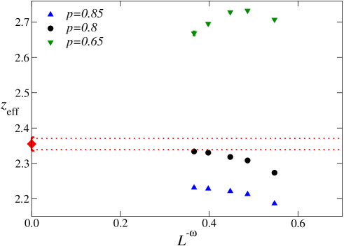
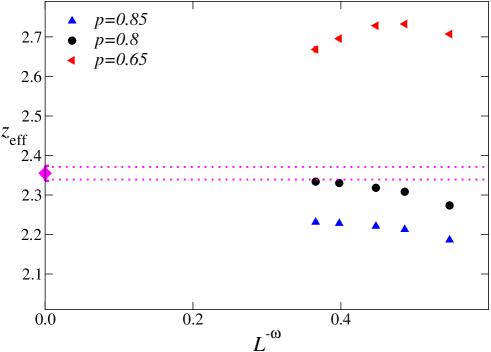
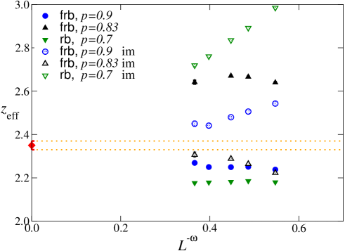
see (26). In Fig. 1 we show $z_{\rm eff}(L)$ as obtained from the estimates of $\tau_{x=1}(L)$ for the RSIM at $p=0.85,0.8,0.65$, reported in Table 2. The raw data show significant scaling corrections and it is far from clear that their limit for $L\to\infty$ is independent of $p$.

In the following we present a detailed analysis of the MC data for the RSIM. First, we analyse the data at $p=0.8$. If the FT description is correct, we should observe a fast convergence to the infinite-volume limit, with corrections proportional to $L^{-\omega_{2}}$. The results presented in Sec. 4.2.1 confirm this prediction. In particular, there is no evidence of a correction-to-scaling exponent smaller than $\omega_{2}$ in dynamic quantities. These results support the general FT scenario which predicts that the two leading correction-to-scaling exponents are the static ones $\omega$ and $\omega_{2}$. Then, we assume the FT scenario and perform a consistency check, verifying that the large differences observed in Fig. 1 can be explained by scaling corrections. To make the check more quantitative, we introduce an improved estimator for the exponent $z$ (we use here the same strategy employed in [6] for static quantities) and show that it converges to the same value obtained for $p=0.8$ with the expected scaling corrections. This allows us to confirm universality, i.e. the $p$ independence of the dynamic critical behaviour.

4.2.1 Analysis at $p=0.8$.

Figure 2: The effective exponent $z_{\rm eff}(L)$ and the corresponding improved quantities $z_{\rm im}(L)$ and $z_{\rm im2}(L)$ defined in (52) versus $L^{-\omega_{2}}$ with $\omega_{2}=0.82$. Results for the RSIM at $p=0.8$. The effective exponents are obtained by using $\tau_{x}(L)$ with $x=1$. The dotted lines correspond to the results of fits to $z+aL^{-0.82}$ with $L_{\rm min}=12$.

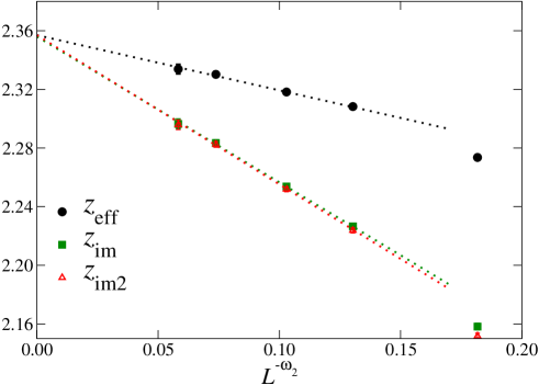
Let us first analyse $\tau_{x}(L)$ for the RSIM at $p=0.8$. If the standard FT description of the model-A dynamics holds, the static correction-to-scaling exponents are the most relevant ones. Since the RSIM at $p=0.8$ is improved, the $O(L^{-k\omega})$ scaling corrections are suppressed and therefore we expect the dominant scaling corrections to be proportional to $L^{-\omega_{2}}$ with $\omega_{2}=0.82(8)$. In Fig. 2 we plot $z_{\rm eff}(L)$ as obtained from $\tau_{x=1}(L)$ versus $L^{-0.82}$. The data with $L\geq 12$ clearly fall on a line. To determine $z$ we assume $\tau_{x}(L)$ to behave as

$$\tau_{x}(L)=cL^{z}\left(1+c_{2}L^{-\varepsilon}\right)$$ (29)

for $L\to\infty$, and perform fits of the form

$$\ln\tau_{x}(L)=z\ln L+\ln c+c_{2}e^{-\varepsilon\ln L},$$ (30)

with $\varepsilon=0.82,0.74,0.90$, which correspond to $\omega_{2}=0.82(8)$. Results for $x=0.6,1,1.5,2$ are shown in Fig. 3 versus $L_{\rm min}$, the smallest lattice size used in the fit. They are independent of $L_{\rm min}$ for $L_{\rm min}\geq 12$, with $\chi^{2}/{\rm DOF}\mathrel{\hbox to0.0pt{\lower 3.0pt\hbox{$\mathchar 536\relax$}\hss}\raise 2.0pt\hbox{$\mathchar 316\relax$}}1$ (DOF is the number of degrees of freedom of the fit). For example, for $x=1$ and $\varepsilon=0.82$, we obtain $z=2.357(4)$ and $c=0.0525(10)$ for $L_{\rm min}=12$, and $z=2.356(6)$ and $c=0.0526(15)$ for $L_{\rm min}=16$. For $x=0.6,1.5,2$, $\varepsilon=0.82$, and $L_{\rm min}=12$, we obtain $z=2.354(3)$, $z=2.356(7)$ and $z=2.358(13)$. One can also estimate $z$ by fitting $z_{\rm eff}(L)$ to $z+e_{21}L^{-\omega_{2}}$. If we determine $z_{\rm eff}(L)$ from $\tau_{x=1}(L)$, we obtain $z=2.357(4)$ for $L_{\rm min}=12$ and $z=2.357(6)$ for $L_{\rm min}=16$. All results are perfectly consistent. From these analyses we obtain the estimate

$$z=2.356(6)[3],$$ (31)

which is the result of the fit of $\tau_{x=1}(L)$ with $\varepsilon=0.82$ and $L_{\rm min}=16$. The error in brackets gives the variation of the estimate as $\omega_{2}$ varies within one error bar.

Figure 3: Estimates of the dynamic exponent $z$ for the RSIM at $p=0.8$ obtained from fits of $\tau_{x}(L)$ to (30) and of the effective exponents to $z+aL^{-\varepsilon}$. We report results corresponding to different values of $L_{\rm min}$: $L_{\rm min}=8,12,16,24$ (some data are slightly shifted along the $x$ axis to make them visible). The dotted lines correspond to the estimate (55), $z=2.355(16)$.

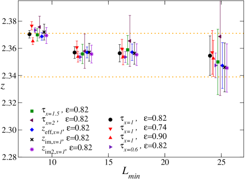
In the above-reported determination we have implicitly assumed that the RSIM at $p=0.8$ is exactly improved so that there are no leading scaling corrections. However, $p^{*}$ is only known approximately and thus some residual $O(L^{-\omega})$ scaling correction are still present. To determine their relevance, we exploit the fact that ratios of leading scaling-correction amplitudes are universal and use the bound [6]

$$|c_{{\cal O},11}(p=0.8)/c_{{\cal O},11}(p=0.65)|\mathrel{\hbox to0.0pt{\lower 3.0pt\hbox{$\mathchar 536\relax$}\hss}\raise 2.0pt\hbox{$\mathchar 316\relax$}}1/30,$$ (32)

which holds for any quantity ${\cal O}$, be it static or dynamic, computed in the RSIM at $p=0.8$ and $p=0.65$ ($c_{{\cal O},11}$ is the amplitude of the $L^{-\omega}$ correction appearing in the large-$L$ behaviour of ${\cal O}$). Bound (32) shows that $\tau_{x}(p=0.8;L)^{1+k}\tau_{x}(p=0.65;L)^{-k}$ is exactly improved (the leading correction proportional to $L^{-\omega}$ exactly cancels) for some $k$ satisfying $|k|\leq 1/30$. Thus, an upper bound on the systematic error due to the $L^{-\omega}$ scaling corrections is obtained by analyzing

$$\tau_{x}(p=0.8;L)^{1\pm 1/30}\times\tau_{x}(p=0.65;L)^{\mp 1/30},$$ (33)

instead of $\tau_{x}(p=0.8;L)$. The estimate of $z$ varies by $\pm 0.008$, which represents the systematic error due to the residual $L^{-\omega}$ corrections. The final result is therefore

$$z=2.356(6)[3]\{8\}.$$ (34)

Figure 4: Estimates of $z_{\rm eff}(L)$, as obtained from $\tau_{x}(L)$ for several values of $x$, for the RSIM at $p=0.8$. The dotted lines correspond to the result $z=2.355(16)$, see (55).

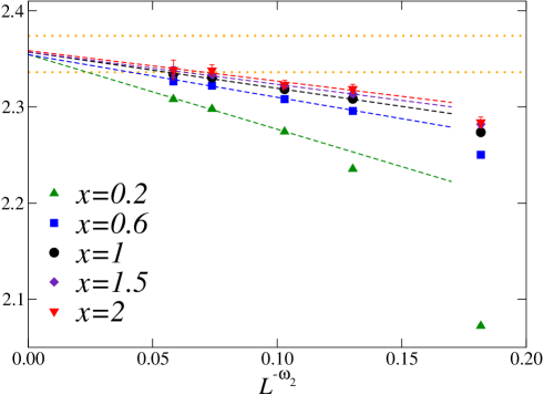
The above-presented analysis shows that the estimates of $z$ obtained by using $\tau_{x}$ with different values of $x$ are perfectly consistent, as of course should be expected. There is therefore little advantage in considering many values of $x$ and it is simpler to restrict the analyses to a single $x$. We wish to choose it in such a way to minimize scaling corrections and statistical errors. As is clear from Table 1 statistical errors decrease with decreasing $x$. In Fig. 4 we show $z_{\rm eff}(L)$ as computed from $\tau_{x}$ for different values of $x$. Scaling corrections decrease with increasing $x$ and are essentially independent of $x$ for $x\mathrel{\hbox to0.0pt{\lower 3.0pt\hbox{$\mathchar 536\relax$}\hss}\raise 2.0pt\hbox{$\mathchar 318\relax$}}1$. Thus, a good compromise between small statistical errors and small scaling corrections is obtained by taking $x$ neither too small nor too large. We have thus chosen $x=1$. The quantities that are analysed in the following sections are always obtained from $\tau_{x=1}(L)$.

4.2.2 Analysis for $p=0.65$ and $p=0.85$.

Let us now consider the RSIM at $p=0.65$ and $p=0.85$. Since the model is not improved we must include corrections with exponent $\omega$ and $2\omega$ at least, i.e. consider correction-to-scaling terms proportional to $L^{-\omega}\approx L^{-0.29}$ and $L^{-2\omega}\approx L^{-0.58}$, which decrease slower than the leading correction term $L^{-\omega_{2}}=L^{-0.82}$ occurring in improved models. Assuming this type of corrections, we fitted $\tau_{x=1}(L)$ with the ansätze

$$\tau_{x=1}(L)=cL^{z}\;\;,$$ (35)

$$\tau_{x=1}(L)=cL^{z}\;(1+c_{11}L^{-\omega})$$ (36)

and

$$\tau_{x=1}(L)=cL^{z}\;(1+c_{11}L^{-\omega}+c_{12}L^{-2\omega})\;\;,$$ (37)

fixing $\omega=0.29$.

Let us first discuss the case $p=0.65$. Fits to (35) give $\chi^{2}/{\rm DOF}\approx 1$ (DOF is the number of degrees of freedom of the fit) starting from $L_{\rm min}=32$. For $L_{\rm min}=32$ we obtain $z=2.671(5)$. Fits to (36) give $\chi^{2}/{\rm DOF}\approx 1$ starting from $L_{\rm min}=24$. For $L_{\rm min}=24$ we obtain $z=2.46(2)$. Fits to (37) have $\chi^{2}/$DOF close to one already for $L_{\rm min}=12$. For $L_{\rm min}=12$ and $L_{\rm min}=16$ we obtain $z=2.31(3)$ and $z=2.23(6)$, respectively.

The same analysis can be repeated for $p=0.85$. If we consider the smallest $L_{\rm min}$ corresponding to $\chi^{2}/$DOF close to 1 for each fit ansatz, we obtain $z=2.229(1)$ (fit to (35), $L_{\rm min}=24$), $z=2.33(3)$ (fit to (36), $L_{\rm min}=12$), and $z=2.12(2)$ (fit to (37), $L_{\rm min}=8$). Again, the results of fits to (37) vary significantly with $L_{\rm min}$: for $L_{min}=12$ we obtain $z=2.21(8)$.

Using the simple power-law ansatz (35) one obtains results that apparently indicate non-universal, $p$-dependent values of $z$. Including the expected corrections to scaling the results for the critical dynamic exponent $z$ change rather dramatically, indicating that scaling corrections play a crucial role in the analysis. However, since the results obtained for $z$ depend strongly on the number of correction terms included in the fit and also on the minimal lattice size $L_{\rm min}$, we cannot obtain a direct accurate estimate of $z$ at these values of $p$. Analogously, it is not possible to include the additional correction term $c_{21}L^{-\omega_{2}}\sim L^{-0.82}$, which was important for the analysis at $p=0.8$ (in this case we should also consider the equivalent correction $L^{-3\omega}\sim L^{-0.87}$). For these reasons, we do not quote a final result for $z$ at $p=0.65$ and $0.85$.

4.2.3 Correction-to-scaling amplitudes.

Figure 5: Difference $\Delta z(p;L)\equiv z_{\rm eff}(p;L)-z_{\rm eff}(p=0.8;L)$ versus $L^{-\omega}$ with $\omega=0.29$ for the RSIM at $p=0.85,0.65$. The dotted lines are the results of fits to $aL^{-\omega}$ in the case of $p=0.65$, and to $aL^{-\omega}+bL^{-2\omega}$ for $p=0.85$.

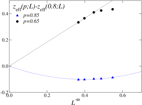
Here we assume that the value of $z$ is universal, i.e. that it does not depend on $p$. Based on this assumption, we compute amplitude ratios that involve the correction amplitude $e_{11}$ defined in (28) and verify that these ratios do not depend on the chosen value of $p$. This provides a consistency check that the dynamic universality class is independent of $p$. This type of analysis is equivalent in spirit to an analysis in which data at different values of $p$ are fitted together assuming the same dynamic exponent $z$. For instance, this is what was done in [5]. There are, however, two significant differences: first, we use the static correction-to-scaling exponents (this allows us to consider the leading and the subleading scaling correction); second, we verify that the amplitudes of the leading scaling correction satisfy the constraints imposed by the RG, i.e. we verify the universality of the amplitude ratios.

For this purpose we consider

$$\Delta z(p;L)\equiv z_{\rm eff}(p;L)-z_{\rm eff}(p=0.8;L).$$ (38)

For $L\to\infty$ it behaves as

$$z_{\rm eff}(p;L)-z_{\rm eff}(p=0.8;L)\approx\bar{e}_{11}L^{-\omega}+\bar{e}_{12}L^{-2\omega}+\cdots+\bar{e}_{21}L^{-\omega_{2}}+\cdots$$ (39)

if the dynamic critical behaviour does not depend on $p$. Since the RSIM at $p=0.8$ is approximately improved, we have $e_{11}\approx 0$ for $p=0.8$, so that

$$\bar{e}_{11}\approx e_{11}(p).$$ (40)

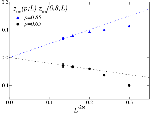
In Fig. 5 we show the difference (39) as obtained from the available data. Fits of $\Delta z(p;L)$ to $aL^{-\omega}$ and $aL^{-\omega}+bL^{-\varepsilon}$ with $\varepsilon=2\omega,\omega_{2}$ provide estimates of $e_{11}$. We obtain $e_{11}=0.9(2)$ at $p=0.65$ and $e_{11}=-0.55(15)$ at $p=0.85$. As expected, corrections have opposite sign in the two cases and are quite significant at the present values of $L$. Note that at $p=0.85$ only fits with two corrections give a reasonable $\chi^{2}$, indicating that at least two correction terms must be taken into account.

Then, we consider the static quartic cumulants

$$U_{22}\equiv{\overline{\mu_{2}^{2}}-\overline{\mu_{2}}^{2}\over\overline{\mu_{2}}^{2}},\qquad U_{4}\equiv{\overline{\mu_{4}}\over\overline{\mu_{2}}^{2}},\qquad U_{d}\equiv U_{4}-U_{22},$$ (41)

where $\mu_{k}\equiv\langle\;(\sum_{x}\sigma_{x}\;)^{k}\rangle$, at fixed $\xi/L=0.5943$—we call them $\bar{U}_{22}$, $\bar{U}_{4}$, and $\bar{U}_{d}$, respectively. For $L\to\infty$ they behave as

$$\bar{U}_{\#}=\bar{U}_{\#}^{*}+c_{\#,11}L^{-\omega}+\ldots,$$ (42)

where [6] $\bar{U}_{22}^{*}=0.148(1)$, $\bar{U}_{4}^{*}=1.648(3)$, and $\bar{U}_{d}^{*}=1.500(1)$. The ratios of the leading scaling-correction amplitudes are universal. In the case of $\bar{U}_{22}$ and $\bar{U}_{d}$, we have [6]

$$s_{c}={c_{22,11}\over c_{d,11}}=-0.44(3).$$ (43)

Analogously, the ratio

$$s_{\#}\equiv{e_{11}\over c_{\#,11}}$$ (44)

is expected to be universal if the dynamic universality class is independent of $p$. The ratios (44) can be directly estimated by considering

$$S_{\#}(p;L)\equiv{z_{\rm eff}(p;L)-z_{\rm eff}(p=0.8;L)\over\bar{U}_{\#}(p;2L)-\bar{U}_{\#}(p=0.8;2L)}=2^{\omega}s_{\#}+b_{1}L^{-\omega}+b_{2}L^{-\omega_{2}+\omega}+\cdots$$ (45)

In Fig. 6 we show $S_{22}$ and $S_{d}$ for $p=0.85,0.65$. At $p=0.65$ a fit of the data with $L\geq 16$ to $a+bL^{-\omega}$ ($\omega=0.29$) gives $s_{22}=9(1)$ and $s_{d}=-4.5(5)$. At $p=0.85$, the same fit gives $s_{22}=7.4(9)$ and $s_{d}=-4.2(5)$. The agreement is satisfactory, taking also into account that the errors do not take into account several sources of systematic uncertainty. The approximate $p$-independence of the ratios $s_{22}$ and $s_{d}$ represents a nontrivial check that the dynamic universality class is independent of $p$. Assuming universality, we obtain for the RSIM

$$s_{d}=-4.5(5),\qquad s_{22}=9(2).$$ (46)

Note that these ratios are consistent with $s_{d}/s_{22}=s_{c}=-0.44(3)$, cf. (43).

Figure 6: Ratios $S_{22}(p;L)$ and $S_{d}(p;L)$ defined in (45) for $p=0.85,0.65$, versus $L^{-\omega}$, $\omega=0.29$.

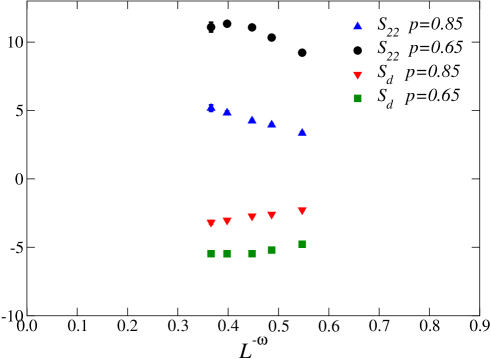
It is interesting to note that the scaling corrections occurring in $\tau_{x}(L)$ are significantly larger than those occurring in static quantities. For instance, we have

$${c_{11}\over(c_{\#,11}/\bar{U}_{\#}^{*})}={s_{\#}U_{\#}^{*}\ln 2\over 2^{-\omega}-1}\approx\cases{-5(1)&for $\bar{U}_{22}$\cr 26(3)&for $\bar{U}_{d}$,}$$ (47)

where $c_{11}$ is defined in (26).

4.2.4 Improved estimators and universality.

In the estimate of $z$ obtained at $p=0.8$ in Sec. 4.2.1, cf. (34), the residual $O(L^{-\omega})$ scaling corrections are an important source of error. These corrections can be significantly reduced by considering improved estimators [6]. The estimate of the universal ratio $s_{d}$ obtained in Sec. 4.2.3 allows us to define improved quantities with smaller $L^{-\omega}$ scaling corrections. Let us consider the quantities

$$Z_{1}(r;L)\equiv z_{\rm eff}(L)\left(\bar{U}_{d}(2L)/\bar{U}_{d}^{*}\right)^{r},\qquad$$

$$Z_{2}(q;L)\equiv z_{\rm eff}(L)+q(\bar{U}_{d}(2L)-\bar{U}_{d}^{*}).$$ (48)

For $L\to\infty$ they behave as

$$Z_{i}(L)=z+f_{11}L^{-\omega}+f_{12}L^{-2\omega}+\cdots+f_{21}L^{-\omega_{2}}+\cdots.$$ (49)

where the correction-to-scaling amplitudes depend on $r$ or $q$. Then, we determine $r^{*}$ and $q^{*}$ such that $f_{11}(r^{*})=f_{11}(q^{*})=0$. An easy calculation gives

$$r^{*}=-{2^{\omega}\bar{U}_{d}^{*}s_{d}\over z},\qquad q^{*}=-2^{\omega}s_{d}.$$ (50)

Note that $r^{*}$ and $q^{*}$ are expressed in terms of universal quantities and thus $Z_{1}(r^{*};L)$ and $Z_{2}(q^{*};L)$ are improved in any model in the same dynamic universality class. Using $s_{d}=-4.5(5)$, $z=2.36(2)$, $\bar{U}_{d}^{*}=1.500(1)$, we obtain

$$r^{*}=3.5(5),\qquad q^{*}=5.5(7).$$ (51)

The error is mostly due to the error on $s_{d}$. For $r=r^{*}$ and $q=q^{*}$ the scaling corrections are proportional to $L^{-2\omega}$ with $2\omega=0.58(4)$. In the following, we define improved estimators by taking the central values of the estimates (51):

$$z_{\rm im}(L)\equiv Z_{1}(r=3.5;L),\qquad z_{\rm im2}(L)\equiv Z_{2}(q=5.5;L).$$ (52)

One may define analogous improved operators by using $\bar{U}_{22}$ instead of $\bar{U}_{d}$. Those defined in terms of $\bar{U}_{d}$ are more convenient because $\bar{U}_{d}^{*}$ is known with better numerical precision. Since $r^{*}$ and $q^{*}$ are known only approximately, $z_{\rm im}(L)$ and $z_{\rm im2}(L)$ still have $L^{-\omega}$ corrections. Taking into account the uncertainty on the estimates of $r^{*}$ and $q^{*}$, we obtain the bound

$$|f_{11}/e_{11}|\mathrel{\hbox to0.0pt{\lower 3.0pt\hbox{$\mathchar 536\relax$}\hss}\raise 2.0pt\hbox{$\mathchar 316\relax$}}1/6,$$ (53)

i.e. the leading scaling correction in $z_{\rm im}(L)$ and $z_{\rm im2}(L)$ is at least a factor of 6 smaller than that occurring in $z_{\rm eff}(L)$.

Figure 7: Effective exponents $z_{\rm eff}(L)$ (above) and $z_{\rm im}(L)$ (below) versus $L^{-\omega}$, $\omega=0.29$, for the RSIM at $p=0.65,0.8,0.85$. The dotted lines correspond to the final result $z=2.355(16)$.

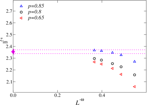
In Fig. 2 we show estimates of $z_{\rm im}(L)$ and $z_{\rm im2}(L)$ at $p=0.8$. Fits to $z+cL^{-\omega_{2}}$ give results in perfect agreement with those obtained by fitting $\tau_{x}(L)$ and $z_{\rm eff}(L)$, see Fig. 3. Note that the data for $z_{\rm im}(L)$ and $z_{\rm im2}(L)$ are very close and provide almost equal results. This can be easily explained by noting that

$$z_{\rm im}(L)-z_{\rm im2}(L)=\left(r-qU_{d}^{*}/z\right)bL^{-\omega_{2}}+\cdots,$$ (54)

where $b$ is a $p$-dependent coefficient. Since $r$ and $q$ are good approximations of $r^{*}$ and $q^{*}$ defined in (50), the prefactor is very small, explaining why the two quantities behave identically. It is interesting to note that $z_{\rm im}(L)$ has $L^{-\omega_{2}}$ corrections which are larger than those occurring in $z_{\rm eff}(L)$, see Fig. 2: improved quantities have smaller leading scaling corrections but larger subleading ones.

In the following we only report results for $z_{\rm im}(L)$. Fits of $z_{\rm im}(L)$ at $p=0.8$ give $z=2.355(8)$ [$z=2.356(7)$] for $L_{\rm min}=16$ [$L_{\rm min}=12$], where the errors also take into account the uncertainty on $\bar{U}_{d}^{*}=1.500(1)$. These results vary approximately by $\pm 0.008$ when changing $\omega_{2}$ within $[0.74,0.90]$, corresponding to the uncertainty on $\omega_{2}$. We finally obtain the estimate

$$z=2.355(8)[8].$$ (55)

Because of the bound (53), the error due to the residual $L^{-\omega}$ scaling corrections is negligible. This result confirms the one given in (34).

Figure 8: Difference $\Delta z_{\rm im}(p;L)\equiv z_{\rm im}(p;L)-z_{\rm im}(p=0.8;L)$ versus $L^{-2\omega}$ with $\omega=0.29$ for the RSIM at $p=0.85,0.65$. The dotted lines correspond to fits to $aL^{-2\omega}$.

In Fig. 7 we report $z_{\rm im}(L)$ and $z_{\rm eff}(L)$ for the three values of $p$ we have considered. In all cases, the improved exponents are quite close to the final estimate (55). For $p=0.85$, while $z_{\rm eff}(L)$ was close to 2.25, $z_{\rm im}(L)$ is fully consistent with 2.355. As for $p=0.65$, the difference between $z_{\rm im}(L)$ and 2.355 is three times smaller than that between $z_{\rm eff}(L)$ and 2.355. The still existing discrepancies can be explained by the next-to-leading $O(L^{-2\omega})$ scaling corrections, as shown by Fig. 8 where the difference $\Delta z_{\rm im}(p;L)\equiv z_{\rm im}(p;L)-z_{\rm im}(p=0.8;L)$ is plotted versus $L^{-2\omega}$. Clearly, $\Delta z_{\rm im}(p;L)$ is consistent with zero, for both $p=0.85$ and $0.65$, if we only consider data with $L\geq 16$, supporting universality.

In conclusion, the results of the RSIM provide an accurate estimate of the dynamic exponent $z$, i.e. $z=2.355(16)$, and a robust evidence of universality, i.e. independence on $p$.

Finally, we note that the leading amplitude $c$ defined in (26) significantly increases with decreasing $p$. Indeed, we find $c\approx 0.03,0.05,0.3$ for $x=1$ and $p=0.85,0.8,0.65$, respectively.

4.3 Universality of $z$ in the RBIM and $\pm J$ Ising model

Figure 9: The effective exponents $z_{\rm eff}(L)$ and $z_{\rm im}(L)$ for the RBIM (rb) at $p=0.55$ and for the $\pm J$ Ising model (frb) at $p=0.883$, versus $L^{-\omega_{2}}$ with $\omega_{2}=0.82$.

We now check the universality of the dynamic exponent $z$ in other RDIs systems, such as the RBIM and the $\pm J$ Ising model along the paramagnetic-ferromagnetic transition line. We first focus on the approximately improved models, the RBIM at $p=0.55$ (the RBIM is improved for $p=p^{*}=0.54(2)$) and the $\pm J$ Ising model at $p=0.883$ (improvement occurs for $p=p^{*}=0.883(3)$). We perform an analysis analogous to that presented for the RSIM at $p=0.8$, verifying that scaling corrections decay as $L^{-\omega_{2}}$, as expected on the basis of field theory, and computing for each of them an estimate of $z$. Then, we verify that the results for the other values of $p$ are consistent with universality, i.e. that the large observed deviations can be interpreted as scaling corrections.

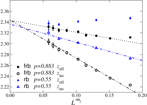
In Fig. 9 we plot $z_{\rm eff}(L)$, defined in (27), and $z_{\rm im}(L)$, defined in (52), versus $L^{-\omega_{2}}$ with $\omega_{2}=0.82$. In the case of the $\pm J$ Ising model, both $z_{\rm eff}(L)$ and $z_{\rm im}(L)$ clearly show the expected $L^{-\omega_{2}}$ behaviour. In the case of the RBIM, $z_{\rm im}(L)$ shows a clear linear trend, while $z_{\rm eff}(L)$ becomes essentially flat as $L$ increases and is close to the RSIM estimate $z=2.355(16)$: indeed, $z_{\rm eff}(L)=2.341(1)$, 2.336(2), 2.338(4) for $L=16,24,32$.

Figure 10: The ratio $\tau_{x=1}(p;L)/\tau_{x=1}({\rm RSIM},p=0.8;L)$ for the RBIM (denoted by rb) at $p=0.55$ and for the $\pm J$ Ising model (frb) at $p=0.883$, versus $L^{-\omega_{2}}$ with $\omega_{2}=0.82$. The dots are the results of fits to $a+cL^{-0.82}$.

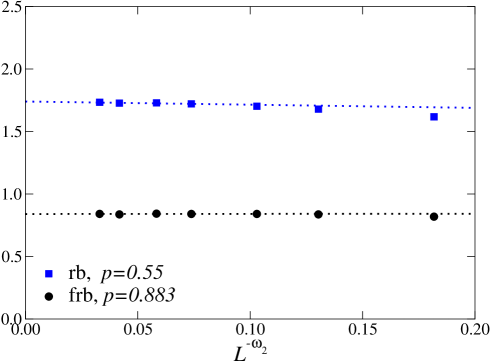
To verify that the RBIM at $p=0.55$ and the $\pm J$ model at $p=0.883$ have the same dynamical critical behaviour as the RSIM at $p=0.8$, in Fig. 10 we plot the ratio

$$\tau_{x=1}(L)/\tau_{x=1}(L)_{{\rm RSIM},p=0.8}.$$ (56)

As $L\to\infty$ the data clearly approach a constant, indicating that all autocorrelation times diverge with the same $z$. The data shown in the figure are well fitted to $b+b_{2}L^{-\omega_{2}}$, with $b\approx 1.74$ and $b\approx 0.84$ respectively for the RBIM and $\pm J$ Ising model.

Figure 11: Estimates of the dynamic exponent $z$ from fits of $\tau_{x=1}(L)$ to (30) with $\varepsilon=0.82$, and of the corresponding $z_{\rm eff}(L)$ and $z_{\rm im}(L)$ to $z+cL^{-0.82}$. The data refer to the $\pm J$ Ising model at $p=0.883$. Some data are slightly shifted along the $x$ axis to make them visible. The dotted lines correspond to the final estimate $z=2.345(17)$, see (58).

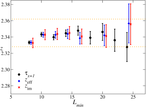
The results of the fits of $\tau_{x=1}(L)$, $z_{\rm eff}(L)$, and $z_{\rm im}(L)$ for the $\pm J$ Ising model at $p=0.883$ are shown in Fig. 11. In particular, by fitting $\tau_{x=1}(L)$ to (30) with $\varepsilon=0.82$, we obtain $z=2.345(4)$ and $c=0.0466(8)$ for $L_{\rm min}=14$. The fit of $z_{\rm eff}(L)$ to $z+eL^{-\omega_{2}}$ gives $z=2.344(6)$ for $L_{\rm min}=14$ and $z=2.342(13)$ for $L_{\rm min}=20$. These results suggest the estimate $z=2.345(4)[3]$. The error in brackets gives the variation of the estimate as $\omega_{2}$ varies by one error bar. By fitting $z_{\rm im}(L)$ to $z+eL^{-\omega_{2}}$ with $\omega_{2}=0.82$, we obtain $z=2.345(8)$ (for $L_{\rm min}=14$), where the error includes the uncertainty on $\bar{U}_{d}^{*}$. The uncertainty on $\omega_{2}$ changes the estimate by $\pm 0.006$.

As in the case of the RSIM, $p^{*}$ is only known approximately and thus some residual leading scaling corrections may still be present. To determine their relevance, we again exploit the fact that ratios of amplitudes of leading scaling corrections are universal, and the bound [7]

$$|c_{{\cal O},11}(p=0.883)/c_{{\cal O},11}(p=0.9)|\mathrel{\hbox to0.0pt{\lower 3.0pt\hbox{$\mathchar 536\relax$}\hss}\raise 2.0pt\hbox{$\mathchar 316\relax$}}1/5.$$ (57)

The error on the estimate obtained from $z_{\rm eff}(L)$ due to possible residual $L^{-\omega}$ scaling corrections can be estimated as in the case of the RSIM at $p=0.8$, obtaining $\pm 0.015$. This error is significantly smaller when $z_{\rm im}(L)$ is considered: the estimate varies by $\pm 0.003$. In conclusion the most precise estimate of $z$ for the $\pm J$ Ising model is obtained by using $z_{\rm im}(L)$. We quote

$$z=2.345(8)[6]\{3\},$$ (58)

which is in good agreement with the RSIM result (55).

Let us now consider the RBIM at $p=0.55$. By fitting $z_{\rm im}(L)$ we obtain $z=2.336(7)$ for $L_{\rm min}=12$, and $z=2.335(9)$ for $L_{\rm min}=16$. We obtain $z=2.335(9)[4]$, where the error in bracket gives the change in the estimate as $\omega_{2}$ varies by one error bar. As in the case of the RSIM and the $\pm J$ Ising model, we must also estimate the error due to the residual $L^{-\omega}$ scaling corrections. Using the results reported in [6], we find that these corrections can at most change the estimate of $z$ by $\pm 0.005$. Our final result is therefore

$$z=2.335(9)[4]\{5\}\;.$$ (59)

In Fig. 12 we show $z_{\rm eff}(L)$ for other values of $p$, i.e. for the RBIM at $p=0.7$ and for the $\pm J$ Ising model at $p=0.83,0.90$. They are plotted versus $L^{-\omega}$, which is the expected leading scaling corrections. As it was observed for the RSIM, see Fig. 1, the results appear strongly $p$-dependent and it is not clear from the data that $z_{\rm eff}(L)$ has a model- and $p$-independent limit as $L\to\infty$. In any case, we can show that these data are still consistent with universality if the expected scaling corrections are taken into account. Let us again consider the difference

$$\Delta z_{\rm RS}(p;L)=z_{\rm eff}(p;L)-z_{\rm eff}({\rm RSIM},p=0.8;L),$$ (60)

which, as discussed in the preceding section, should behave as

$$\Delta z_{\rm RS}(p;L)\approx\bar{e}_{1}(p)L^{-\omega}+\bar{e}_{2}L^{-\varepsilon},$$ (61)

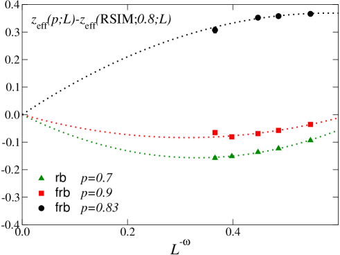
with $\varepsilon=2\omega,\omega_{2}$ for $L\to\infty$. We recall that $\bar{e}_{1}\approx e_{11}$, cf. (28). In order to show consistency with universality, we fit $\Delta z_{\rm RS}(p;L)$ to the ansatz (61), determining $e_{11}$. Then, we consider $\bar{U}_{22}$ and determine the leading correction-to-scaling amplitude $c_{22,11}$ defined in (42). Finally, we verify that the ratio $s_{22}\equiv e_{11}/c_{22,11}$ is independent of $p$ and of the model, and that it agrees with the RSIM estimate (46), $s_{22}=9(2)$.

Figure 12: Effective exponents $z_{\rm eff}(L)$ and $z_{\rm im}(L)$ for the RBIM at $p=0.7$ (rb) and the $\pm J$ Ising model at $p=0.83,0.90$ (frb). The dotted lines correspond to the final estimate $z=2.35(2)$.

As shown in Fig. 13, good fits of $\Delta z_{\rm RS}(p;L)$ to (61) are obtained by taking $\varepsilon=2\omega$. They give $\bar{e}_{1}=-1.0(2)$ for the RBIM at $p=0.7$, and $\bar{e}_{1}=1.2(2),-0.5(1)$ for the $\pm J$ Ising model at $p=0.83,0.9$, respectively. The amplitude $c_{22,11}$ can be estimated analogously. We obtain $c_{22,11}=-0.17(3),\,0.10(2),\,-0.05(1)$, respectively for the RBIM at $p=0.7$, and the $\pm J$ Ising model at $p=0.83,0.9$. These results give

$$s_{22}=6(2),\;\;12(3),\;\;10(3),$$ (62)

which are in substantial agreement with the estimate (46) obtained from the RSIM. These results fully support the interpretation of the anomalous behaviour of the data shown in Figs. 12 and 13 as an effect of scaling corrections.

Figure 13: The difference $\Delta z_{\rm RS}(p;L)\equiv z_{\rm eff}(p;L)-z_{\rm eff}({\rm RSIM},p=0.8;L)$ versus $L^{-\omega}$ with $\omega=0.29$ for the RBIM (rb) and the $\pm J$ Ising model (frb). The dotted lines are the results of the fits to $aL^{-\omega}+bL^{-2\omega}$.

Figure 14: The difference $z_{\rm im}(p;L)-2.35$ versus $L^{-2\omega}$ with $\omega=0.29$ for the RBIM (rb) and the $\pm J$ Ising model (frb).

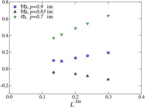
In Fig. 12 we also show $z_{\rm im}(L)$. For the $\pm J$ model at $p=0.83$, the improved estimator is significantly closer to $z\approx 2.35$ than $z_{\rm eff}(L)$. In the two other cases deviations are still large, though the data seem to approach faster the limiting value $z\approx 2.35$ obtained by considering the improved models. In Fig. 14 we show the difference $z_{\rm im}(L)-2.35$ versus $L^{-2\omega}$, which would be the leading scaling correction if $z_{\rm im}(L)$ were exactly improved. The data for the $\pm J$ Ising model converge to zero, confirming universality. On the other hand, the RBIM data apparently extrapolate to a slightly positive value. However, if we include an additional correction term (either an $L^{-\omega}$ term, since improvement is only approximate, or an $L^{-\omega_{2}}$ term), the data are again perfectly consistent with universality.

4.4 Summary of the results for the equilibrium relaxational dynamics at $T_{c}$

In this section we have studied the Metropolis equilibrium dynamics in the RSIM, the RBIM, and the $\pm J$ Ising model along the paramagnetic-ferromagnetic transition line, which belong to the same static universality class. We have verified that the exponent $z$ is the same for the RSIM, the RBIM, and the $\pm J$ Ising model for values of the disorder parameter $p$ that make these models approximately improved. We have obtained $z=2.355(16)$, $z=2.335(18)$, and $z=2.345(17)$ respectively for the RSIM at $p=0.8$, the RBIM at $p=0.55$, and the $\pm J$ Ising model at $p=0.883$. For the other values of $p$ we have not been able to determine $z$ with comparable precision. We have however verified that the dynamic behaviour is always consistent with universality once the expected scaling corrections are taken into account. In the analyses we have presented, scaling corrections play a very important role. We have explicitly verified the FT prediction that dynamics does not introduce new RG irrelevant operators that are more relevant than the two leading ones occurring in the statics. Therefore, scaling corrections are characterized by the same universal exponents that control the nonasymptotic behaviour in static quantities, i.e. $\omega=0.29(2)$ and $\omega_{2}=0.82(8)$. As a consequence, the leading $L^{-k\omega}$ scaling corrections are absent in dynamic observables at the same value $p^{*}$ of the disorder parameter $p$ determined by considering static quantities.

Once universality has been checked, we can use our results for the RSIM, the RBIM, and the $\pm J$ Ising model, to obtain a final estimate for $z$. We quote

$$z=2.35(2),$$ (63)

which includes all results obtained in the previous sections.

Our result (63) significantly improves earlier MC estimates [18, 19, 23] of $z$ obtained in equilibrium MC simulations. Reference [19] considered several values of $p$ in the range $1>p\geq 0.6$. The final estimate $z=2.4(1)$ was essentially derived from the data at $p=0.8$, where the finite-size behaviour appeared least dependent on $L$. The different values of $z$ obtained for other values of $p$ were interpreted as a crossover phenomenon. A smaller estimate $z=2.2(1)$ was found in [23], by MC simulations at $p=0.85$. This may be explained by the effect of scaling corrections, which, as shown by Fig. 1, give rise to an apparent smaller value of $z$ if they are not taken into account.

5 Off-equilibrium estimate of the dynamic critical exponent $z$

The exponent $z$ can also be determined by performing off-equilibrium simulations [30, 31, 16]. One starts from a disordered configuration and observes the relaxation at $T_{c}$ on sufficiently large lattices. In the infinite-volume limit the magnetic susceptibility $\chi$ is expected to increase with the MC time $t$ as

$$\chi(t)=C_{0}t^{\rho}\left(1+C_{11}t^{-\upsilon_{1}}+C_{12}t^{-2\upsilon_{1}}+\cdots+C_{21}t^{-\upsilon_{2}}+\cdots\right),$$ (64)

where

$$\rho={2-\eta\over z}.$$ (65)

Using the estimate obtained in Sec. 4, $z=2.35(2)$, and [6] $\eta=0.036(1)$, we predict $\rho=0.836(7)$. Moreover, according to the FT perturbative analysis [30, 31, 16], the leading scaling-correction exponents should be the same as those that occur in equilibrium (static or dynamic) correlation functions. Therefore, we expect

$$\upsilon_{1}={\omega\over z}=0.123(9),\qquad\upsilon_{2}={\omega_{2}\over z}=0.35(3),$$ (66)

where we have used $\omega=0.29(2)$ and $\omega_{2}=0.82(8)$. Moreover, the leading scaling correction proportional to $t^{-\upsilon_{1}}$ (and also all corrections of the form $t^{-k\upsilon_{1}}$) vanishes in improved models.

Equation (64) is valid only in the infinite-volume limit. For a finite system of size $L$ we expect

$$\chi(t,L)=C_{0}\,t^{\rho}\,E_{0}(tL^{-z})(1+C_{11}t^{\upsilon_{1}}E_{1}(tL^{-z})+\cdots)$$ (67)

where $E_{i}(x)$ are universal functions satisfying $E_{i}(0)=1$ and $E_{0}(x)\sim x^{-\rho}$, $E_{1}(x)\sim x^{\upsilon_{1}}$ for large $x$.

The off-equilibrium relaxational dynamics of the RSIM has already been investigated in [20, 22] for various values of $p$ in the range $1>p\geq 0.4$. Their results do not agree with the above-reported predictions. References [20, 22] obtain $z=2.62(7)$ and $z=2.6(1)$, respectively, independently of the dilution parameter $p$. They also estimate the leading correction-to-scaling exponent $\upsilon_{1}$. Given their estimate of $z$, this allows them to estimate $\omega$. They quote $\omega=0.50(13)$ and $\omega=0.61(6)$, respectively. It is quite difficult to reconcile these results with the FT predictions; in particular, the absence of corrections proportional to $t^{-0.12}$, i.e. controlled by the leading exponent $\omega=0.29(2)$, is quite surprising. Another numerical MC work [21] investigated the nonequilibrium relaxation dynamics of the $\pm J$ Ising model, and showed an apparent non-universal dynamical critical behaviour along the paramagnetic-ferromagnetic transition line. Also these results are in contrast with the FT predictions reported at the beginning of section.

In the following we further investigate this issue. We study the Metropolis dynamics of the RSIM at $p=0.8$ after a quench from $T=\infty$ to $T_{c}$. This represents a nontrivial check of the FT predictions, since the estimates (65) and (66) are quite precise. Since the model is approximately improved [$p^{*}=0.800(5)$], we expect that $C_{1k}$ vanishes for all values of $k$, and thus we predict

$$\chi(t)=C_{0}t^{\rho}\left(1+C_{21}t^{-\upsilon_{2}}+\cdots\right),$$ (68)

$$\rho=0.836(7),\qquad\upsilon_{2}=0.35(3).$$

As in the equilibrium case, we define an effective exponent

$$\rho_{\rm eff}(t)\equiv{\ln[\chi(2t)/\chi(t)]\over\ln 2},$$ (69)

which behaves as

$$\rho_{\rm eff}(t)=\rho+ct^{-\upsilon_{2}}+\ldots$$ (70)

for $t\to\infty$. On a finite lattice, (70) is replaced by

$$\rho_{\rm eff}(t,L)=\rho+e_{0}(tL^{-z})$$ (71)

where we have neglected large-$t$ (scaling) corrections and $e_{0}(x)$ is a universal function (apart from a normalization of the argument) such that $e_{0}(0)=0$ and $e_{0}(x)\to-\rho$ for $x\to\infty$.

Figure 15: Effective exponent $\rho_{\rm eff}(t,L)$ for $L=64,96,128$. Here $t$ is the number of MC sweeps.

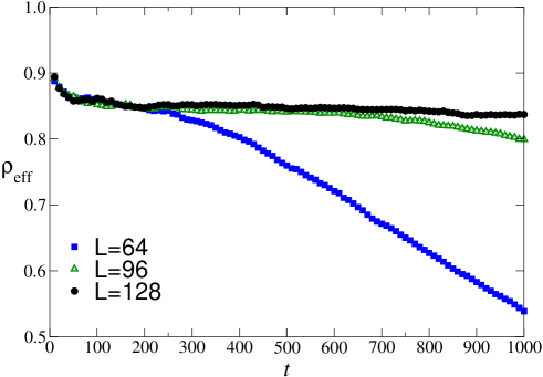
We have performed off-equilibrium MC simulations on lattices of size $L=64,96,128$ at $\beta=0.2857430$ [our presently best estimate of $\beta_{c}$ is $\beta=0.2857431(3)$]. For each lattice size we average over $N_{s}=320000$ disorder configurations. For each disorder configuration we start from a (different) $T=\infty$ configuration and perform 2000 Metropolis sweeps, using the algorithm described in Sec. 4.1 and B. In Fig. 15 we show $\rho_{\rm eff}(t,L)$ for $L=64,96,128$. It clearly shows finite-size corrections, and, for each $L$, $\rho_{\rm eff}(t,L)$ follows the infinite-volume curve up to an $L$-dependent value $t_{\rm max}(L)$. As shown by Fig. 16, where $\rho_{\rm eff}(t,L)$ is plotted versus $t_{\rm resc}\equiv t(L/128)^{-z}$, finite-size effects are consistent with (71). Thus, the value $t_{\rm max}(L)$, after which finite-size effects cannot be neglected, increases as $L^{z}$. Infinite-volume quantities, such as $\rho_{\rm eff}(t)$, must be obtained from the data at $t<t_{\rm max}(L)$. Fig. 15 indicates that, with the statistical errors of our data, $t_{\rm max}(L)\approx 120,600$ for $L\approx 64,128$. Since $\rho_{\rm eff}(t,L)$ is defined using data at $t$ and $2t$, this implies that, for $L=128$, only data corresponding to $t\mathrel{\hbox to0.0pt{\lower 3.0pt\hbox{$\mathchar 536\relax$}\hss}\raise 2.0pt\hbox{$\mathchar 316\relax$}}1200$ have negligible finite-size effects within our error bars. Finite-size effects give rise to a systematic error in the estimate of $\rho$. As is clear from Fig. 15, they yield smaller values of $\rho$, and therefore larger values of $z$.

Figure 16: The effective exponent $\rho_{\rm eff}(t,L)$ versus $t_{\rm resc}=t(L/128)^{-z}$.

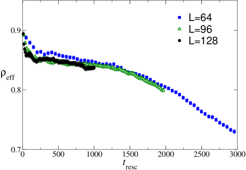
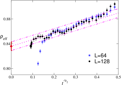
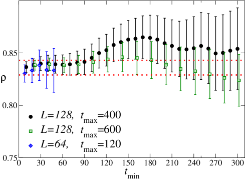
In Fig. 17 we plot $\rho_{\rm eff}(t,L)$ for $L=64,128$ versus $t^{-\upsilon_{2}}$ with $\upsilon_{2}=0.35$. Finite-size effects are negligible for $t^{-\upsilon_{2}}>t_{\rm max}(L)^{-\upsilon_{2}}\approx 0.17,0.10$, for $L=64,128$, respectively. The data satisfying this inequality clearly follow a unique curve, which is expected to behave as $\rho+ct^{-\upsilon_{2}}$ for sufficiently large values of $t$. The data plotted in Fig. 17 clearly show such a behaviour in the region $t^{-\upsilon_{2}}\mathrel{\hbox to0.0pt{\lower 3.0pt\hbox{$\mathchar 536\relax$}\hss}\raise 2.0pt\hbox{$\mathchar 316\relax$}}0.4$ (corresponding to $t\mathrel{\hbox to0.0pt{\lower 3.0pt\hbox{$\mathchar 536\relax$}\hss}\raise 2.0pt\hbox{$\mathchar 318\relax$}}10$), and are perfectly compatible with the values $\rho=0.836(7)$ and $\upsilon_{2}=0.35(2)$. This is also shown by Fig. 18, where we plot the results of fits of $\rho_{\rm eff}(t,L)$ for $t_{\rm min}\leq t\leq t_{\rm max}$ to $\rho+ct^{-\upsilon_{2}}$ with $\upsilon_{2}=0.35$, for $L=64,128$.

The above results provide a nice check of the results of the previous section and confirm the RG prediction that the off-equilibrium relaxational critical dynamics is characterized by the same dynamic exponent $z$ and the same scaling-correction exponents $\omega$ and $\omega_{2}$ as the equilibrium critical dynamics. Note that the results of Fig. 17 rule out the larger estimates of $z$ obtained in [20, 22], $z=2.62(7)$ and $z=2.6(1)$, corresponding to $\rho=0.750(20)$ and $\rho=0.755(29)$, respectively (using [6] $\eta=0.036(1)$).

Figure 17: Effective exponent $\rho_{\rm eff}(t,L)$ versus $t^{-\upsilon_{2}}$ with $\upsilon_{2}=0.35$. Finite-size effects are negligible for $t^{-\upsilon_{2}}\mathrel{\hbox to0.0pt{\lower 3.0pt\hbox{$\mathchar 536\relax$}\hss}\raise 2.0pt\hbox{$\mathchar 318\relax$}}0.10$ ($L=128$) and $t^{-\upsilon_{2}}\mathrel{\hbox to0.0pt{\lower 3.0pt\hbox{$\mathchar 536\relax$}\hss}\raise 2.0pt\hbox{$\mathchar 318\relax$}}0.17$ ($L=64$). The lines are drawn to guide the eyes.

Figure 18: Results of fits of $\rho_{\rm eff}(t,L)$ for $t_{\rm min}\leq t\leq t_{\rm max}$ to $\rho+ct^{-\upsilon_{2}}$ with $\upsilon_{2}=0.35$, for $L=64,128$. The dotted lines correspond to the prediction $\rho=0.836(7)$ obtained by using the equilibrium result $z=2.35(2)$ and $\eta=0.036(1)$ [6].

6 Conclusions

In this paper we have studied the purely relaxational dynamics (model A) in randomly diluted Ising (RDIs) systems. According to standard RG arguments applied to dynamics, the dynamic critical behaviour in such systems should belong to the same model-A dynamic universality class. If this description is correct, the dynamic exponent $z$ is the same in all RDIs systems and the leading scaling corrections are controlled by the same RG operators that appear in the statics and therefore are characterized by the static correction-to-scaling exponents $\omega=0.29(2)$ and $\omega_{2}=0.82(8)$. For the same reasons, in the case of improved Hamiltonians, leading scaling corrections should also be absent in dynamical quantities. Therefore, improved models are expected to provide the most precise estimates of universal dynamic quantities. For instance, in FSS studies at the critical point, corrections to scaling decay as $L^{-0.82}$ in improved models, while in generic RDIs systems the approach to the infinite-volume limit is much slower, corrections decaying as $L^{-0.29}$.

The main results of our analysis can be summarized as follows.

• We consider the RSIM at $p=0.8$, the RBIM at $p=0.55$, and the $\pm J$ Ising model at $p=0.833$, at the critical point. These three models are approximately improved (the best estimates of $p^{*}$, the value of the disorder parameter corresponding to an improved model, are 0.800(5), 0.54(2), 0.833(3) in the three models, respectively [6, 7]). We perform high-statistics equilibrium MC simulations on lattices $L^{3}$, $L\leq 64$, using the Metropolis algorithm (for the RSIM and the RBIM a small modification is needed to ensure ergodicity, see B). We determine the exponent $z$, obtaining $z=2.355(16)$ for the RSIM, $z=2.335(18)$ for the RBIM, and $z=2.345(17)$ for the $\pm J$ Ising model. These results are in perfect agreement, providing strong support to the FT prediction that all RDIs models belong to the same dynamic model-A universality class. We also investigate in detail the scaling corrections: they are perfectly consistent with a behaviour of the form $L^{-\omega_{2}}$, with $\omega_{2}=0.82(8)$. Again this is in agreement with the FT analysis. Our final result is

  $$z=2.35(2).$$ (72)

  Note that, while we confirm the general scenario predicted by field theory, there is a quantitative difference between our result and that obtained by resumming the perturbative expansions at two and three loops, $z\approx 2.18$ [28, 29]. This may be due to a poor convergence of the perturbative FT expansions. The apparent agreement with the $O(\sqrt{\epsilon})$ result [24] $z=2+\sqrt{6\epsilon/53}$, which would give $z\approx 2.336$ for $\epsilon=1$, is likely only by chance.

• We investigate the Metropolis dynamics in equilibrium in the RSIM, the RBIM, and in the $\pm J$ Ising model for other values of $p$. Here, as expected, corrections are very strong. In the FSS analysis, the leading term is expected to decay as $L^{-\omega}$, $\omega=0.29(2)$. We are not able to determine $z$ in these models as accurately as in improved models. In any case we verify that the $L$-behaviour of the MC data at $T_{c}$ is consistent with universality and with the constraints imposed by the RG (universality of ratios of correction-to-scaling amplitudes).

• We have no evidence of two different universality classes depending on the disorder strength [44, 45]. In particular, we show that the critical behavior is not influenced by the geometrical structure of the vacancies and does not depend whether the vacancies percolate or not. Indeed, since site and bond vacancies percolate for $p\mathrel{\hbox to0.0pt{\lower 3.0pt\hbox{$\mathchar 536\relax$}\hss}\raise 2.0pt\hbox{$\mathchar 316\relax$}}0.688$ and $p\mathrel{\hbox to0.0pt{\lower 3.0pt\hbox{$\mathchar 536\relax$}\hss}\raise 2.0pt\hbox{$\mathchar 316\relax$}}0.751$, respectively, in the improved RSIM ($p=0.8$) vacancies form finite clusters, while in the improved RBIM ($p=0.55$) vacancies percolate. Nonetheless, the critical behavior is the same.

• The results for the $\pm J$ Ising model show that frustration is irrelevant for the relaxational behaviour along the paramagnetic-ferromagnetic transition line. It is worth mentioning that this is not true for the cluster dynamics. In that case the exponent $z$ in the $\pm J$ Ising model is much larger than in the RSIM and RBIM. In the frustrated case we obtained $z\approx 1.6$ [7], while in the second one simulations indicate $z\mathrel{\hbox to0.0pt{\lower 3.0pt\hbox{$\mathchar 536\relax$}\hss}\raise 2.0pt\hbox{$\mathchar 316\relax$}}0.5$ [23].

• We investigate the off-equilibrium relaxational dynamics in the RSIM at $p=0.8$. We start from disordered $T=\infty$ configurations and observed the relaxation at $T=T_{c}$. The results show that our equilibrium estimate $z=2.35(2)$ is perfectly consistent with the off-equilibrium MC data. In the analysis particular care has been taken to avoid finite-size corrections. Moreover, the large-time scaling corrections are consistent with what is expected on the basis of field theory [30, 31, 16]. Since the model is improved, we do not observe corrections proportional to $t^{-\omega/z}$; instead our data show corrections that are proportional to $t^{-\omega_{2}/z}$. Here $\omega$ and $\omega_{2}$ are the static correction-to-scaling exponents, $\omega=0.29(2)$ and $\omega_{2}=0.82(8)$.

The relaxational critical behaviour within the RDIs universality class is also relevant for the so-called model-C dynamics, where the order parameter couples with a conserved secondary density [11]. In the case of the 3D RDIs universality class, the asymptotic critical behaviours of the model-A and model-C dynamics are described by the same stable fixed point. Therefore, they are expected to have the same dynamic exponent $z$. This is essentially related to the fact that the specific-heat exponent of RDIs systems, $\alpha=-0.049(6)$, is negative [46]. A drastic change occurs in the approach to the asymptotic behaviour, which is expected to be much slower in model C [47]. The coupling with a conserved scalar density gives rise to very slowly decaying $O(\xi^{-\omega_{c}},L^{-\omega_{c}})$ scaling corrections with

$$\omega_{c}={3\over 2}-{1\over\nu}=-{\alpha\over 2\nu}=0.036(4),$$ (73)

which is much smaller than the leading scaling-correction exponent of the model-A dynamics, which is $\omega=0.29(2)$.

Appendix A Estimate of the leading correction-to-scaling exponent $\omega$

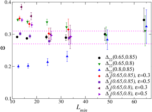
In this appendix we compute the leading correction-to-scaling exponent $\omega$. We use the method discussed in [6] and combine the data of [6] with those obtained here. We consider the quartic cumulants $\bar{U}_{22}$ and $\bar{U}_{d}$, cf. (41), at fixed $\xi/L=0.5943$, at $p=0.85,0.8.0.65$ on lattices of size $L\leq 192$.

As in [6], in order to estimate $\omega$, we consider the differences

$$\Delta_{22}(p_{1},p_{2};L)\equiv\bar{U}_{22}(p_{1};L)-\bar{U}_{22}(p_{2};L),$$ (74)

$$\Delta_{d}(p_{1},p_{2};L)\equiv\bar{U}_{d}(p_{1};L)-\bar{U}_{d}(p_{2};L).$$ (75)

Universality implies that

$$\Delta\approx c_{\Delta,11}L^{-\omega}+c_{\Delta,12}L^{-2\omega}+\cdots+c_{\Delta,21}L^{-\omega_{2}}+\cdots$$ (76)

In the case of $\Delta_{22}$, fits to $cL^{-\omega}$ provide good and stable results. In the case of $\Delta_{d}$, an additional correction term is needed in order to obtain an acceptable $\chi^{2}$. Hence, we fit $\Delta_{d}$ to $c_{1}L^{-\omega}+c_{2}L^{-\varepsilon}$. In Fig. 19 we show the results as a function of $L_{\rm min}$, the minimum lattice size used in the fit. They become independent of $p_{1}$, $p_{2}$, and of the considered quantity as $L_{\rm min}$ increases. The most stable results are obtained by taking $p_{1}=0.85$ and $p_{2}=0.65$. From the results shown in Fig. 19, we obtain the estimate

$$\omega=0.29(2).$$ (77)

This estimate is more precise than previous ones and is consistent with $\omega=0.33(3)$ obtained in [6] by using part of the data at $p=0.65$ and $p=0.8$. For comparison, the FT six-loop result [9] is $\omega=0.25(10)$ (we also mention the five-loop result $\omega=0.32(6)$ of [10]).

Figure 19: Estimates of the leading correction-to-scaling exponent $\omega$. The dotted lines correspond to our final result $\omega=0.29(2)$.

Appendix B Metropolis algorithm for randomly diluted Ising models

We have implemented the standard local Metropolis algorithm with the acceptance rate

$$A=\mbox{min}[1,\exp(-\beta[\cal{H}^{\prime}-\cal{H}])],$$ (78)

where $\cal{H}^{\prime}$ and $\cal{H}$ correspond to the Hamiltonian evaluated for the proposal and for the given spin configuration, respectively. The proposal is generated by flipping the sign of the spin at a single site $x$ of the lattice. Hence $\cal{H}^{\prime}-\cal{H}$ depends only on the values of the spins at the site $x$ and at its neighbours $y$.

To speed up the simulation we use multispin coding (see, e.g., [48]), evolving in parallel $n_{\rm bit}$ systems ($n_{\rm bit}=64$ in our case). For each of them we use a different set of disorder variables. The implementation in the RSIM and RBIM is more complicated than in the standard Ising model and the $\pm J$ Ising model, since the sum over the nearest neighbours assumes one of the 13 values $\{-6,-5,...,5,6\}$ and not only the 7 even values $\{-6,-4,...,4,6\}$.

We perform the single-site update sequentially, moving from one site to one of its neighbours in a typewriter fashion. This causes problems with ergodicity. This can be understood by considering the isolated lattice sites, i.e. the sites $x$ such that $\rho_{y}=0$ (RSIM) or $J_{<xy>}=0$ (RBIM) for all neighbours $y$. For an isolated site the difference $\cal{H}^{\prime}-\cal{H}$ always vanishes, so that, using the acceptance rate (78), the proposal is always accepted. Hence, going through the lattice twice, the spins on the isolated sites go back to their values. Therefore, the configuration restricted to the isolated sites is not changed. Note that the problem is not restricted to isolated sites only. For example, for the one-dimensional chain one can easily prove that a regular update sweep using the acceptance rate (78) is not ergodic. There are many ways to avoid this problem. For performance reason, we prefer to update the spins sequentially. To avoid the problem the spin flip is proposed with probability $w$ strictly smaller than one. We have chosen $w=0.9$. Note that the problem occurs only in the RSIM and in the RBIM. For the $\pm J$ Ising model the standard Metropolis update can be used.

References

- [1] Belanger D P, Experimental characterization of the Ising model in disordered antiferromagnets, 2000, Braz. J. Phys. 30 682, arXiv:cond-mat/0009029
- [2] Pelissetto A and Vicari E, Critical phenomena and renormalization-group theory, 2002, Phys. Rept. 368 549, arXiv:cond-mat/0012164
- [3] Folk R, Holovatch Yu and Yavors’kii T, Critical exponents of a three dimensional weakly diluted quenched Ising model, 2003, Uspekhi Fiz. Nauk 173 175 [English translation 2003, Phys. Usp. 46 169], arXiv:cond-mat/0106468
- [4] Janke W, Berche B, Chatelain C, Berche P E and Hellmund M, Quenched disordered ferromagnets, 2005, PoS(LAT2005)018
- [5] Ballesteros H G, Fernández L A, Martín-Mayor V, Muñoz Sudupe A, Parisi G and Ruiz-Lorenzo J J, Critical exponents of the three dimensional diluted Ising model, 1998, Phys. Rev.B 58 2740, arXiv:cond-mat/9802273
- [6] Hasenbusch M, Parisen Toldin F, Pelissetto A and Vicari E, Universality class of 3D site-diluted and bond-diluted Ising systems , 2007, JSTAT P02016, arXiv:cond-mat/0611707
- [7] Hasenbusch M, Parisen Toldin F, Pelissetto A and Vicari E, Critical behavior of the three-dimensional Ising model at the paramagnetic-ferromagnetic transition line, 2007, Phys. Rev. B 76 094402, arXiv:0704.0427 [cond-mat.dis-nn]
- [8] Calabrese P, Martín-Mayor V, Pelissetto A and Vicari E, The three-dimensional randomly dilute Ising model: Monte Carlo results, 2003, Phys. Rev.E 68 036136, arXiv:cond-mat/0306272
- [9] Pelissetto A and Vicari E, Randomly dilute spin models: a six-loop field-theoretic study, 2000, Phys. Rev.B 62 6393, arXiv:cond-mat/0002402
- [10] Pakhnin D V and Sokolov A I, Critical exponents for a three-dimensional impure Ising model in the five-loop approximation, 2000, Pis’ma v Zh. Eksp. Teor. Fiz. 71 600 [reprinted in 2000, JETP Letters, 71 412]Pakhnin D V and Sokolov A I, Five-loop renormalization-group expansions for the three-dimensional n-vector cubic model and critical exponents for impure Ising systems, 2000, Phys. Rev.B 61 15130, arXiv:cond-mat/9912071
- [11] Hohenberg P C and Halperin B I, Theory of dynamic critical phenomena, 1977, Rev. Mod. Phys. 49 435
- [12] Rosov N, Hohenemser C and Eibschütz M, Dynamic critical behavior of the random-exchange Ising system Fe0.9Zn0.1F2 determined via Mössbauer spectroscopy, 1992, Phys. Rev.B 46 3452
- [13] Belanger D P, Farago B, Jaccarino V, King A R, Lartigue C and Mezei F, Random exchange Ising model dynamics: Fe0.46Zn0.54F2, Proceedings of the Intern. Conf. on Magnetism (ICM), Paris, 1988, Givord D ed., 1988, J. Phys. (Paris) Colloq. 49 C8-1229
- [14] Barrett P H, Static and dynamic critical phenomena in Fe1-xZnxF2, 1986, Phys. Rev.B 34 3513
- [15] Janssen H K, Oerding K and Sengespeick E, On the crossover to universal criticality in dilute Ising systems, 1995, J. Phys. A: Math. Gen.28 6073
- [16] Calabrese P and Gambassi A, Ageing properties of critical systems, 2005, J. Phys. A: Math. Gen.38 R133, arXiv:cond-mat/0410357
- [17] Folk R and Moser G, Critical dynamics: a field-theoretical approach, 2006, J. Phys. A: Math. Gen.39 R207
- [18] Prudnikov V V and Vakilov A N, Numerical simulation of the critical dynamics of dilute magnetic materials, 1992, Pis’ma v Zh. Eksp. Teor. Fiz. 55 709 [English translation 1992, JETP Letters 55 741]Prudnikov V V and Vakilov A N, Computer simulation of the critical dynamics in diluted magnets, 1992, Zh. Eksp. Teor. Fiz. 103 962 [English translation 1993, JETP 76 469]
- [19] Heuer H-O, Dynamic scaling of disordered Ising systems, 1993, J. Phys. A: Math. Gen.26 L341
- [20] Parisi G, Ricci-Tersenghi F and Ruiz-Lorenzo J J, Universality of the off-equilibrium critical dynamics of the three-dimensional diluted Ising model, 1999, Phys. Rev.E 60 5198, arXiv:cond-mat/9903905
- [21] Ito N, Ozeki Y and Kitatani H, Non-universal critical behaviour in the ferromagnetic transition of the Ising model, 1999, J. Phys. Soc. Jpn. 68 803
- [22] Schehr G and Paul R, Universal aging properties at a disordered critical point, 2005, Phys. Rev.E 72 016105, arXiv:cond-mat/0412447
- [23] Ivaneyko D, Ilnytskyi J, Berche B and Holovatch Yu, Criticality of the random-site Ising model: Metropolis, Swendsen-Wang and Wolff Monte Carlo algorithms, 2006, Cond. Matt. Phys. (Ukraine) 9 319, arXiv:cond-mat/0501291Ivaneyko D, Ilnytskyi J, Berche B and Holovatch Yu, Local and cluster critical dynamics of the 3d random-site Ising model, 2006, Physica A 370 163, arXiv:cond-mat/0603521.
- [24] Grinstein G, Ma S-k and Mazenko G F, Dynamics of spins interacting with quenched random impurities, 1977, Phys. Rev.B 15 258
- [25] De Dominicis C, Dynamics as a substitute for replicas in systems with quenched random impurities, 1978, Phys. Rev.B 18 4913
- [26] Prudnikov V V and Vakilov A N, Critical dynamics of dilute magnets, 1992 Zh. Eksp. Teor. Fiz. 101 1853 [English translation 1992, JETP 74 990]
- [27] Prudnikov V V, Belim S V, Osintsev E V and Fedorenko A A, Critical dynamics of disordered magnets in the three-loop approximation 1998, Fiz. Tverd. Tela (St. Petersburg) 40 1526 [English translation 1998, Phys. Sol. State 40 1383]Prudnikov V V, Belim S V, Ivanov A V, Osintsev E V and Fedorenko A A, Critical dynamics of slightly disordered spin systems, 1998, Zh. Eksp. Teor. Fiz. 114 972 [English translation 1998, JETP 87 527]
- [28] Blavats’ka V, Dudka M, Folk R and Holovatch Yu, Critical dynamics and effective exponents of magnets with extended impurities, 2005, Phys. Rev.B 72 064417, arXiv:cond-mat/0506644
- [29] Prudnikov V V, Prudnikov P V and Krinitsyn A S, Calculations of the dynamical critical exponent using the asymptotic series summation method, 2006, Teor. Mat. Fiz. 147 137 [English translation 2006, Theor. Math. Phys. 147 561], arXiv:cond-mat/0606530
- [30] Janssen H K, Schaub B and Schmittmann B, New universal short-time scaling behaviour of critical relaxation processes, 1989, Z. Phys. B 73 539
- [31] Oerding K and Janssen H K, Nonequilibrium critical relaxation in dilute Ising systems, 1995, J. Phys. A: Math. Gen.28 4271
- [32] Ballesteros H G, Fernández L A, Martín-Mayor V, Muñoz Sudupe A, Parisi G and Ruiz-Lorenzo J J, Scaling corrections: site percolation and Ising model in three dimensions, 1999, J. Phys. A: Math. Gen.32 1, arXiv:cond-mat/9805125
- [33] Lorenz C D and Ziff R M, Precise determination of the bond percolation thresholds and finite-size scaling corrections for the sc, fcc, and bcc lattices, 1998, Phys. Rev.E 57 230, arXiv:cond-mat/9710044
- [34] Edwards S F and Anderson P W, Theory of spin glasses, 1975, J. Phys. F 5 965
- [35] Hasenbusch M, Parisen Toldin F, Pelissetto A and Vicari E, Magnetic-glassy multicritical behavior of the three-dimensional Ising model, 2007, Phys. Rev.B in press, arXiv:0707.2866 [cond-mat.dis-nn]
- [36] Sokal A D, 1997, Monte Carlo Methods in Statistical Mechanics: Foundations and New Algorithms, in Functional Integration: Basics and Applications, de Witt-Morette C, Cartier P and Folacci A eds., pp. 131-192, New York:Plenum
- [37] Bray A J, Dynamics of dilute magnets above , 1988, Phys. Rev. Lett.60 720
- [38] Griffiths R B, Nonanalytic behavior above the critical point in a random Ising ferromagnet, 1969, Phys. Rev. Lett.23 17Schwartz M, Upper bounds on cluster distribution functions and the nature of the Griffiths singularity, 1978, Phys. Rev.B 18 2364
- [39] Dhar D, Randeria M and Sethna J P, Griffiths singularities in the dynamics of disordered Ising models, 1988, Europhys. Lett. 5 485
- [40] Bray A J, Upper and lower bounds on dynamic correlations in the Griffiths phase, 1989, J. Phys. A: Math. Gen.22 L81
- [41] Cesi F, Maes C and Martinelli F, Relaxation of disordered magnets in the Griffiths’ regime, 1998, Comm. Math. Phys. 188 135
- [42] Madras N and Sokal A D, The pivot algorithm: A highly efficient Monte Carlo method for the self-avoiding walk, 1988, J. Stat. Phys. 50 109
- [43] Ballesteros H G, Fernández L A, Martín-Mayor V, Muñoz Sudupe A, Parisi G and Ruiz-Lorenzo J J, The four dimensional site-diluted Ising model: a finite-size scaling study, 1998, Nucl. Phys. B 512 681, arXiv:hep-lat/9707017.
- [44] Murtazaev A K, Kamilov I K and Babaev A B, Critical behavior of a cubic lattice 3 D Ising model for systems with quenched disorder, 2004, Zh. Eksp. Teor. Fiz. 126 1377 [English translation 2004, JETP 99 1201]
- [45] Prudnikov V V, Prudnikov P V, Vakilov A N and Krinitsyn A S, Computer simulation of the critical behavior of 3 D disordered Ising model, 2004, Zh. Eksp. Teor. Fiz. 132 [English translation 2007, JETP 105 371], arXiv:0709.1450 [cond-mat.dis-nn]
- [46] Halperin B I, Hohenberg P C and Ma S-k, Renormalization-group methods for critical dynamics: I. Recursion relations and effects of energy conservation, 1974, Phys. Rev.B 10 139Halperin B I, Hohenberg P C and Ma S-k, Renormalization-group methods for critical dynamics: II. Detailed analysis of the relaxational models, 1976, Phys. Rev.B 13 4119
- [47] Dudka M, Folk R, Holovatch Yu and Moser G, Critical dynamics of diluted relaxational models coupled to a conserved density, 2005, Phys. Rev.E 72 036107, arXiv:cond-mat/0506325 Dudka M, Folk R, Holovatch Yu and Moser G, Model C critical dynamics of disordered magnets, 2006, J. Phys. A: Math. Gen.39 7943, arXiv:cond-mat/0601262
- [48] Wansleben S, Zabolitzky J B and Kalle C, Monte Carlo simulation of Ising models by multispin coding on a vector computer, 1984, J. Stat. Phys. 37 271Bhanot G, Duke D and Salvador R, Finite-size scaling and the three-dimensional Ising model, 1986, Phys. Rev.B 33 7841