A Bayesian Approach to Network Modularity

Abstract

We present an efficient, principled, and interpretable technique for inferring module assignments and for identifying the optimal number of modules in a given network. We show how several existing methods for finding modules can be described as variant, special, or limiting cases of our work, and how the method overcomes the resolution limit problem, accurately recovering the true number of modules. Our approach is based on Bayesian methods for model selection which have been used with success for almost a century, implemented using a variational technique developed only in the past decade. We apply the technique to synthetic and real networks and outline how the method naturally allows selection among competing models.

Large-scale networks describing complex interactions among a multitude of objects have found application in a wide array of fields, from biology to social science to information technology Albert and Barabási (2002); Watts and Strogatz (1998). In these applications one often wishes to model networks, suppressing the complexity of the full description while retaining relevant information about the structure of the interactions Ziv et al. (2005). One such network model groups nodes into modules, or “communities,” with different densities of intra- and inter- connectivity for nodes in the same or different modules. We present here a computationally efficient Bayesian framework for inferring the number of modules, model parameters, and module assignments for such a model.

The problem of finding modules in networks (or “community detection”) has received much attention in the physics literature, wherein many approaches Newman and Girvan (2004); Reichardt and Bornholdt (2006) focus on optimizing an energy-based cost function with fixed parameters over possible assignments of nodes into modules. The particular cost functions vary, but most compare a given node partitioning to an implicit null model, the two most popular being the configuration model and a limited version of the stochastic block model (SBM) Holland and Leinhardt (1976); McSherry (2001). While much effort has gone into how to optimize these cost functions, less attention has been paid to what is to be optimized. In recent studies which emphasize the importance of the latter question it was shown that there are inherent problems with existing approaches regardless of how optimization is performed, wherein parameter choice sets a lower limit on the size of detected modules, referred to as the “resolution limit” problem Fortunato and Barthélemy (2007); Kumpula et al. (2007). We extend recent probabilistic treatments of modular networks Hastings (2006); Newman and Leicht (2007) to develop a solution to this problem that relies on inferring distributions over the model parameters, as opposed to asserting parameter values a priori, to determine the modular structure of a given network. The developed techniques are principled, interpretable, computationally efficient, and can be shown to generalize several previous studies on module detection.

We specify an $N$-node network by its adjacency matrix $\mathbf{A}$, where $A_{ij}=1$ if there is an edge between nodes $i$ and $j$ and $A_{ij}=0$ otherwise, and define $\sigma_{i}\in\{1,\ldots,K\}$ to be the unobserved module membership of the $i^{\rm th}$ node. We use a constrained SBM, which consists of a multinomial distribution over module assignments with weights $\pi_{\mu}\equiv p(\sigma_{i}=\mu|\vec{\pi})$ and Bernoulli distributions over edges contained within and between modules with weights $\vartheta_{c}\equiv p(A_{ij}=1|\sigma_{i}=\sigma_{j},\vec{\vartheta})$ and $\vartheta_{d}\equiv p(A_{ij}=1|\sigma_{i}\neq\sigma_{j},\vec{\vartheta})$, respectively. In short, to generate a random undirected graph under this model we roll a $K$-sided die (biased by $\vec{\pi}$) $N$ times to determine module assignments for each of the $N$ nodes; we then flip one of two biased coins (for either intra- or inter- module connection, biased by $\vartheta_{c},\vartheta_{d}$, respectively) for each of the $N(N-1)/2$ pairs of nodes to determine if the pair is connected. The extension to directed graphs is straightforward.

Using this model, we write the joint probability $p(\mathbf{A},\vec{\sigma}|\vec{\pi},\vec{\vartheta},K)=p(\mathbf{A}|\vec{\sigma},\vec{\vartheta})p(\vec{\sigma}|\vec{\pi})$ (conditional dependence on $K$ has been suppressed below for brevity) as

$$p(\mathbf{A},\vec{\sigma}|\vec{\pi},\vec{\vartheta})=\vartheta_{c}^{c_{+}}(1-\vartheta_{c})^{c_{-}}\vartheta_{d}^{d_{+}}(1-\vartheta_{d})^{d_{-}}\prod_{\mu=1}^{K}\pi_{\mu}^{n_{\mu}}$$ (1)

where $c_{+}\equiv\sum_{i>j}A_{ij}\delta_{\sigma_{i},\sigma_{j}}$ is the number of edges contained within communities, $c_{-}\equiv\sum_{i>j}(1-A_{ij})\delta_{\sigma_{i},\sigma_{j}}$ is the number of non-edges contained within communities, $d_{+}\equiv\sum_{i>j}A_{ij}(1-\delta_{\sigma_{i},\sigma_{j}})$ is the number of edges between different communities, $d_{-}\equiv\sum_{i>j}(1-A_{ij})(1-\delta_{\sigma_{i},\sigma_{j}})$ is the number of non-edges between different communities, and $n_{\mu}\equiv\sum_{i=1}^{N}\delta_{\sigma_{i},\mu}$ is the occupation number of the $\mu^{\rm th}$ module. Defining $\mathcal{H}\equiv-\ln p(\mathbf{A},\vec{\sigma}|\vec{\pi},\vec{\vartheta})$ and regrouping terms by local and global counts, we recover (up to additive constants) a generalized version of Hastings (2006):

$$\mathcal{H}=-\sum_{i>j}\left(J_{L}A_{ij}-J_{G}\right)\delta_{\sigma_{i},\sigma_{j}}+\sum_{\mu=1}^{K}h_{\mu}\sum_{i=1}^{N}\delta_{\sigma_{i},\mu},$$ (2)

a Potts model Hamiltonian with unknown coupling constants $J_{G}\equiv\ln(1-\vartheta_{d})/(1-\vartheta_{c})$, $J_{L}\equiv\ln{\vartheta_{c}/\vartheta_{d}}+J_{G}$, and chemical potentials $h_{\mu}\equiv-\ln\pi_{\mu}$. (Note that many previous methods omit a chemical potential term, implicitly assuming equally-sized groups.)

While previous approaches Reichardt and Bornholdt (2006); Hastings (2006) minimize related Hamiltonians as a function of $\vec{\sigma}$, these methods require that the user specifies values for these unknown constants, which gives rise to the resolution limit problem Fortunato and Barthélemy (2007); Kumpula et al. (2007). Our approach, however, uses a disorder-averaged calculation to infer distributions over these parameters, avoiding this issue. To do so, we take beta $(\mathcal{B})$ and Dirichlet $(\mathcal{D})$ distributions over $\vec{\vartheta}$ and $\vec{\pi}$, respectively:

$$p(\vec{\vartheta})p(\vec{\pi})\equiv\mathcal{B}(\vartheta_{c};\tilde{c}_{+_{0}},\tilde{c}_{-_{0}})\mathcal{B}(\vartheta_{d};\tilde{d}_{+_{0}},\tilde{d}_{-_{0}})\mathcal{D}(\vec{\pi};\tilde{\vec{n}}_{0}).$$ (3)

These conjugate prior distributions, are defined on the full range of $\vec{\vartheta}$ and $\vec{\pi}$, respectively, and their functional forms are preserved when integrated against the model to obtain updated parameter distributions. Their hyperparameters $\{\tilde{c}_{+_{0}},\tilde{c}_{-_{0}},\tilde{d}_{+_{0}},\tilde{d}_{-_{0}},\tilde{\vec{n}}_{0}\}$ act as pseudocounts that augment observed edge counts and occupation numbers.

In this framework the problem of module detection can be stated as follows: given an adjacency matrix $\mathbf{A}$, determine the most probable number of modules (i.e. occupied spin states) $K^{*}=\mathrm{argmax}_{K}\ p(K|\mathbf{A})$ and infer posterior distributions over the model parameters (i.e. coupling constants and chemical potentials) $p(\vec{\pi},\vec{\vartheta}|\mathbf{A})$ and the latent module assignments (i.e. spin states) $p(\vec{\sigma}|\mathbf{A})$. In the absence of a priori belief about the number of modules, we demand that $p(K)$ is sufficiently weak that maximizing $p(K|\mathbf{A})\propto p(\mathbf{A}|K)p(K)$ is equivalent to maximizing $p(\mathbf{A}|K)$, referred to as the evidence. This approach to model selection Kass and Raftery (1995) proposed by the statistical physicist Jeffreys in 1935 Jeffreys (1935) balances model fidelity and complexity to determine, in this context, the number of modules.

A more physically intuitive interpretation of the evidence is as the disorder-averaged partition function of a spin-glass, calculated by marginalizing over the possible quenched values of the parameters $\vec{\vartheta}$ and $\vec{\pi}$ as well as the spin configurations $\vec{\sigma}$:

$$\mathcal{Z}=p(\mathbf{A}|K) = \sum_{\vec{\sigma}}\int\!\!d\vec{\vartheta}\int\!\!d\vec{\pi}\ p(\mathbf{A},\vec{\sigma}|\vec{\pi},\vec{\vartheta})p(\vec{\vartheta})p(\vec{\pi})$$ (4)

$$= \sum_{\vec{\sigma}}\int\!\!d\vec{\vartheta}\int\!\!d\vec{\pi}\ e^{-\mathcal{H}}p(\vec{\vartheta})p(\vec{\pi}).$$ (5)

While the $\vec{\vartheta}$ and $\vec{\pi}$ integrals in Eqn. 4 can be performed analytically, the remaining sum over module assignments $\vec{\sigma}$ scales as $K^{N}$ and becomes computationally intractable for networks of even modest sizes. To accommodate large-scale networks we use a variational approach that is well-known to the statistical physics community Feynman (1972) and has recently found application in the statistics and machine learning literature, commonly termed variational Bayes (VB) Jordan et al. (1999). We proceed by taking the negative logarithm of $\mathcal{Z}$ and using Gibbs’s inequality:

$$-\ln\mathcal{Z} = -\ln\sum_{\vec{\sigma}}\int\!\!d\vec{\vartheta}\int\!\!d\vec{\pi}\ q(\vec{\sigma},\vec{\pi},\vec{\vartheta}){p(\mathbf{A},\vec{\sigma},\vec{\pi},\vec{\vartheta}|K)\over q(\vec{\sigma},\vec{\pi},\vec{\vartheta})}$$ (6)

$$\leq -\sum_{\vec{\sigma}}\int\!\!d\vec{\vartheta}\int\!\!d\vec{\pi}\ q(\vec{\sigma},\vec{\pi},\vec{\vartheta})\ln{p(\mathbf{A},\vec{\sigma},\vec{\pi},\vec{\vartheta}|K)\over q(\vec{\sigma},\vec{\pi},\vec{\vartheta})}.$$ (7)

That is, we first multiply and divide by an arbitrary approximating distribution $q(\vec{\sigma},\vec{\pi},\vec{\vartheta})$ and then upper-bound the log of the expectation by the expectation of the log. We define the quantity to be minimized – the expression in Eqn. 7 – as the variational free energy $F\{q;\mathbf{A}\}$, a functional of $q(\vec{\sigma},\vec{\pi},\vec{\vartheta})$. (Note that the negative log of $q(\vec{\sigma},\vec{\pi},\vec{\vartheta})$ plays the role of a test Hamiltonian in variational approaches in statistical mechanics.)

We next choose a factorized approximating distribution $q(\vec{\sigma},\vec{\pi},\vec{\vartheta})=q_{\vec{\sigma}}(\vec{\sigma})q_{\vec{\pi}}(\vec{\pi})q_{\vec{\vartheta}}(\vec{\vartheta})$ with $q_{\vec{\pi}}(\vec{\pi})=\mathcal{D}(\vec{\pi};\vec{n})$ and $q_{\vec{\vartheta}}(\vec{\vartheta})=q_{c}(\vartheta_{c})q_{d}(\vartheta_{d})=\mathcal{B}(\vartheta_{c};\tilde{c}_{+},\tilde{c}_{-})\mathcal{B}(\vartheta_{d};\tilde{d}_{+},\tilde{d}_{-})$; as in mean field theory, we factorize $q_{\vec{\sigma}}(\vec{\sigma})$ as $q(\sigma_{i}=\mu)=Q_{i\mu}$, an $N$-by-$K$ matrix which gives the probability that the $i$-th node belongs to the $\mu$-th module. Evaluating $F\{q;\mathbf{A}\}$ with this functional form for $q(\vec{\sigma},\vec{\pi},\vec{\vartheta})$ gives a function of the variational parameters $\{\tilde{c}_{+},\tilde{c}_{-},\tilde{d}_{+},\tilde{d}_{-},\tilde{\vec{n}}\}$ and matrix elements $Q_{i\mu}$ which can subsequently be minimized by taking the appropriate derivatives.

We summarize the resulting iterative algorithm, which provably converges to a local minimum of $F\{q;\mathbf{A}\}$ and provides controlled approximations to the evidence $p(\mathbf{A}|K)$ as well as the posteriors $p(\vec{\pi},\vec{\vartheta}|\mathbf{A})$ and $p(\vec{\sigma}|\mathbf{A})$:

Initialization.—Initialize the $N$-by-$K$ matrix $\mathbf{Q}=\mathbf{Q}_{0}$ and set pseudocounts $\tilde{c}_{+}=\tilde{c}_{+_{0}},\tilde{c}_{-}=\tilde{c}_{-_{0}},\tilde{d}_{+}=\tilde{d}_{+_{0}},\tilde{d}_{-}=\tilde{d}_{-_{0}},$ and $\tilde{n}_{\mu}=\tilde{n}_{\mu_{0}}$.

Main Loop.—Until convergence in $F\{q;\mathbf{A}\}$:

(i) Update the expected value of the coupling constants and chemical potentials

$$\langle J_{L}\rangle = \psi(\tilde{c}_{+})-\psi(\tilde{c}_{-})-\psi(\tilde{d}_{+})+\psi(\tilde{d}_{-})$$ (8)

$$\langle J_{G}\rangle = \psi(\tilde{d}_{-})-\psi(\tilde{d}_{+}+\tilde{d}_{-})$$ (9)

$$-\psi(\tilde{c}_{-})+\psi(\tilde{c}_{+}+\tilde{c}_{-})$$

$$\langle h_{\mu}\rangle = \psi\left(\sum_{\mu}\tilde{n}_{\mu}\right)-\psi(\tilde{n}_{\mu}),$$ (10)

where $\psi(x)$ is the digamma function;

(ii) Update the variational distribution over each spin $\sigma_{i}$

$$Q_{i\mu}\propto\exp\left\{\sum_{j\neq i}\left[\langle J_{L}\rangle A_{ij}-\langle J_{G}\rangle\right]Q_{j\mu}-\langle h_{\mu}\rangle\right\}$$ (11)

normalized such that $\sum_{\mu}Q_{i\mu}=1$, for all $i$;

(iii) Update the variational distribution over parameters from the expected counts and pseudocounts

$$\tilde{n}_{\mu} = \langle n_{\mu}\rangle+\tilde{n}_{\mu_{0}}=\sum_{i=1}^{N}Q_{i\mu}+\tilde{n}_{\mu_{0}}$$ (12)

$$\tilde{c}_{+} = \langle c_{+}\rangle+\tilde{c}_{+_{0}}={1\over 2}Tr(\mathbf{Q}^{T}\mathbf{A}\mathbf{Q})+\tilde{c}_{+_{0}}$$ (13)

$$\tilde{c}_{-} = \langle c_{-}\rangle+\tilde{c}_{-_{0}}$$ (14)

$$= {1\over 2}Tr(\mathbf{Q}^{T}(\vec{u}\langle\vec{n}\rangle^{T}-\mathbf{Q}))-\langle c_{+}\rangle+\tilde{c}_{-_{0}}$$

$$\tilde{d}_{+} = \langle d_{+}\rangle+\tilde{d}_{+_{0}}=M-\langle c_{+}\rangle+\tilde{d}_{+_{0}}$$ (15)

$$\tilde{d}_{-} = \langle d_{-}\rangle+\tilde{d}_{-_{0}}=C-M-\langle c_{-}\rangle+\tilde{d}_{-_{0}},$$ (16)

where $C=N(N-1)/2$, $M=\sum_{i>j}A_{ij}$, and $\vec{u}$ is a $N$-by-$1$ vector of 1’s;

(iv) Calculate the updated optimized free energy

$$F\{q;\mathbf{A}\} = -\ln{\mathcal{Z}_{c}\mathcal{Z}_{d}\mathcal{Z}_{\vec{\pi}}\over\tilde{\mathcal{Z}}_{c}\tilde{\mathcal{Z}}_{d}\tilde{\mathcal{Z}}_{\vec{\pi}}}+\sum_{\mu=1}^{K}\sum_{i=1}^{N}Q_{i\mu}\ln Q_{i\mu},$$ (17)

where $\mathcal{Z}_{\vec{\pi}}={B}(\tilde{\vec{n}})$ is the beta function with a vector-valued argument, the partition function for the Dirichlet distribution $q_{\vec{\pi}}(\vec{\pi})$ (likewise for $q_{c}(\vartheta_{c}),q_{d}(\vartheta_{d})$).

As this provably converges to a local optimum, VB is best implemented with multiple randomly-chosen initializations of $\mathbf{Q}_{0}$ to find the global minimum of $F\{q;\mathbf{A}\}$.

Convergence of the above algorithm provides the approximate posterior distributions $q_{\vec{\sigma}}(\vec{\sigma}),q_{\vec{\pi}}(\vec{\pi})$, and $q_{\vec{\vartheta}}(\vec{\vartheta})$ and simultaneously returns $K^{*}$, the number of non-empty modules that maximizes the evidence. As such, one needs only to specify a maximum number of allowed modules and run VB; the probability of occupation for extraneous modules converges to zero as the algorithm runs and the most probable number of occupied modules remains.

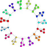
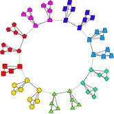
This is significantly more accurate than other approximate methods, such as Bayesian Information Criterion (BIC) Schwarz (1978) and Integrated Classification Likelihood (ICL) Biernacki et al. (2000); Hugo Zanghi and Miele (2007), and is less computationally expensive than empirical methods such as cross-validation (CV) Stone (1974); Airoldi et al. (2007) in which one must perform the associated procedure after fitting the model for each considered value of $K$. Specifically, BIC and ICL are suggested for single-peaked likelihood functions well-approximated by Laplace integration and studied in the large-$N$ limit. For a SBM the first assumption of a single-peaked function is invalidated by the underlying symmetries of the latent variables, i.e. nodes are distinguishable and modules indistinguishable. See Fig. 1 for comparison of our method with the Girvan-Newman modularity Newman and Girvan (2004) in the resolution limit test Fortunato and Barthélemy (2007); Kumpula et al. (2007), where VB consistently identifies the correct number of modules. (Note that VB is both accurate and fast: it performs competitively in the “four groups” test Danon et al. (2005) and scales as $\mathcal{O}(MK)$. Runtime for the main loop in MATLAB on a 2GHz laptop is $\sim\!\!6$ minutes for $N=10^{6}$ nodes with average degree 16 and $K=4$.)

${K_{\rm True}}$	10	11	12	13	14	15	16	17	18	19	20
${K_{\rm VB}}$	10	11	12	13	14	15	16	17	18	19	20
${K_{\rm GN}}$	10	11	12	13	14	8	9	9	10	11	11

Figure 1: Results for the resolution limit test suggested in Fortunato and Barthélemy (2007) and Kumpula et al. (2007). Shapes and colors correspond to the inferred modules. (Left) Our method, variational Bayes, in which all 15 modules are correctly identified (each clique is assigned a unique color/shape). (Right) GN modularity optimization, where failure due to the resolution limit is observed – neighboring cliques are incorrectly grouped together. (Bottom) The results of this test implemented for a range of true number of modules, $K_{\rm true}$, the number of 4-node cliques in the ring-like graph. Note that our method correctly infers the number of communities $K_{\rm VB}$ over the entire range of $K_{\rm True}$, while GN modularity initially finds the correct number of communities but fails for $K_{\rm True}\geq 15$ as shown analytically in Fortunato and Barthélemy (2007).

Furthermore, we note that previous methods in which parameter inference is performed by optimizing a likelihood function via Expectation Maximization (EM) Newman and Leicht (2007); Hugo Zanghi and Miele (2007) are also special cases of the framework presented here. EM is a limiting case of VB in which one collapses the distributions over parameters to point-estimates at the mode of each distribution; however EM is prone to overfitting and cannot be used to determine the appropriate number of modules, as the likelihood of observed data increases with the number of modules in the model. As such, VB performs at least as well as EM while simultaneously providing complexity control Bishop (2006); MacKay (2003).

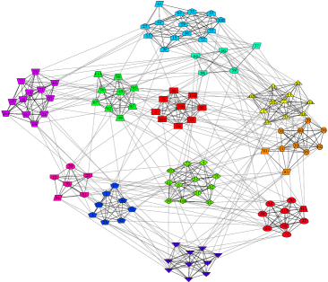
In addition to validating the method on synthetic networks, we apply VB to the 2000 NCAA American football schedule shown in Fig. 2 Girvan and Newman (2002). Each of the 115 nodes represents an individual team and each of the 613 edges represents a game played between the nodes joined. The algorithm correctly identifies the presence of the 12 conferences which comprise the schedule, where teams tend to play more games within than between conferences, making most modules assortative. Of the 115 teams, 105 teams are assigned to their corresponding conferences, with the majority of exceptions belonging to the frequently-misclassified independent teams Clauset et al. (2007) – the only disassortative group in the network. We emphasize that, unlike other methods in which the number of conferences must be asserted, VB determines 12 as the most probable number of conferences automatically.

Figure 2: Each of the 115 nodes represents a NCAA team and each of the 613 edges a game played in 2000 between two teams it joins. The inferred module assignments (designated by color) on the football network which recover the 12 NCAA conferences (designated by shape). Nodes 29, 43, 59, 60, 64, 81, 83, 91, 98, and 111 are misclassified and are mostly independent teams, represented by parallelograms.

Posing module detection as inference of a latent variable within a probabilistic model has a number of advantages. It clarifies what precisely is to be optimized and suggests a principled and efficient procedure for how to perform this optimization. Inferring distributions over model parameters reveals the natural scale of a given modular network, avoiding resolution limit problems. This method allows us to view a number of approaches to the problem by physicists, applied mathematicians, social scientists, and computer scientists as related subparts of a larger problem. In short, it suggests how a number of seemingly-disparate methods may be re-cast and united. A second advantage of this work is its generalization to other models, including those designed to reveal structural features other than modularity. Finally, use of the evidence allows model selection not only among nested models, e.g. models differing only in the number of parameters, but even among models of different parametric families. The last strikes us as a natural area for progress in the statistical study of real-world networks.

It is a pleasure to acknowledge useful conversations on modeling with Joel Bader and Matthew Hastings, on Monte Carlo methods for Potts models with Jonathan Goodman, with David Blei on variational methods, and with Aaron Clauset for his feedback on this manuscript. J.H. was supported by NIH 5PN2EY016586; C.W. was supported by NSF ECS-0425850 and NIH 1U54CA121852.

References

- Albert and Barabási (2002) R. Albert and A.-L. Barabási, Rev. Mod. Phys. 74, 47 (2002).
- Watts and Strogatz (1998) D. J. Watts and S. H. Strogatz, Nature 393, 440 (1998).
- Ziv et al. (2005) E. Ziv, M. Middendorf, and C. H. Wiggins, Phys. Rev. E 71, 046117 (2005).
- Reichardt and Bornholdt (2006) J. Reichardt and S. Bornholdt, Phys. Rev. E 74, 016110 (2006).
- Newman and Girvan (2004) M. Newman and M. Girvan, Phys. Rev. E 69, 026113 (2004).
- Holland and Leinhardt (1976) P. Holland and S. Leinhardt, Sociological Methodology 7, 1 (1976).
- McSherry (2001) F. McSherry, in IEEE Symposium on Foundations of Computer Science (2001), pp. 529–537.
- Kumpula et al. (2007) J. Kumpula, J. Saramäki, K. Kaski, and J. Kertész, Eur. Phys. J. B 56, 41 (2007).
- Fortunato and Barthélemy (2007) S. Fortunato and M. Barthélemy, PNAS 104, 36 (2007).
- Hastings (2006) M. B. Hastings, Phys. Rev. E 74, 035102(R) (2006).
- Newman and Leicht (2007) M. E. J. Newman and E. A. Leicht, PNAS 104, 9564 (2007).
- Kass and Raftery (1995) R. E. Kass and A. E. Raftery, J. Amer. Stat. Assoc. 90, 773 (1995).
- Jeffreys (1935) H. Jeffreys, Proc. Camb. Phil. Soc. 31, 203 (1935).
- Feynman (1972) R. P. Feynman, Statistical Mechanics, A Set of Lectures (W. A. Benjamin, 1972), ISBN 0805325085.
- Jordan et al. (1999) M. I. Jordan, Z. Ghahramani, T. Jaakkola, and L. K. Saul, Machine Learning 37, 183 (1999).
- Schwarz (1978) G. Schwarz, The Annals of Statistics 6, 461 (1978).
- Biernacki et al. (2000) C. Biernacki, G. Celeux, and G. Govaert, IEEE Trans. Pattern Anal. Mach. Intell. 22, 719 (2000).
- Hugo Zanghi and Miele (2007) C. A. Hugo Zanghi and V. Miele, Fast online graph clustering via Erdös-Réyni mixture (2007), sSB-RR-8.
- Airoldi et al. (2007) E. M. Airoldi, D. M. Blei, S. E. Fienberg, and E. P. Xing, Mixed membership stochastic blockmodels (2007).
- Stone (1974) M. Stone, J. Royal Stat. Soc. 36, 111 (1974).
- Danon et al. (2005) L. Danon, A. Díaz-Guilera, J. Duch, and A. Arenas, Journal of Statistical Mechanics: Theory and Experiment p. P09008 (2005).
- Bishop (2006) C. M. Bishop, Pattern recognition and machine learning (Springer, 2006).
- MacKay (2003) D. J. MacKay, Information theory, inference, and learning algorithms (Cambridge University Press, 2003).
- Girvan and Newman (2002) M. Girvan and M. E. J. Newman, PNAS 99, 7821 (2002).
- Clauset et al. (2007) A. Clauset, C. Moore, and M. E. J. Newman, in ICML 2006 Ws, Lecture Notes in Computer Science, edited by E. M. Airoldi (Springer-Verlag, 2007).