Constraining the growth factor with baryon oscillations
Abstract
The growth factor of linear fluctuations is probably one of the least known quantity in observational cosmology. Here we discuss the contraints that baryon oscillations in galaxy power spectra from future surveys can put on a conveniently parametrized growth factor. We find that spectroscopic surveys of 5000 deg2 extending to could estimate the growth index within ; a similar photometric survey would give . This test provides an important consistency check for the standard cosmological model and could constrain modified gravity models. We discuss the errors and the figure of merit for various combinations of redshift errors and survey sizes.
I Introduction
The characterization of dark energy (DE) has been so far based almost uniquely on background tests at rather low redshifts (: Riess et al. 1998, Perlmutter et al. 1999, Tonry et al. 2003, Riess et al. 2004, Astier et al. 2006, Eisenstein et al. 2005) or very large redshifts (: e.g. Netterfield et al. 2002, Halverson et al. 2002, Lee et al. 2002, Bennett et al. 2003, Spergel et al. 2006). These tests are based essentially on estimations of luminosity or angular-diameter distances , i.e. on integrals of the Hubble function which, in turn, contain integrals of the equation of state. Only very recently tests involving the linear perturbations have begun to be discussed, using methods based on the integrated Sachs-Wolfe effect, weak lensing and high-redshift power spectra (e.g. Boughn & Crittenden 2004, Refregier et al. 2006, Crotts et al. 2005 ). However, it is fair to say that the growth function is still one of the least known quantity in cosmology. So far, it is possible to quote only two published results that put limits on it: the value at obtained in 2dF (Hawkins et al. 2003; Verde et al. 2002) and the result from Lyman clouds (McDonald et al. 2005). Defining ( being the matter density contrast) we have for
| (1) |
the value for 2dF at and for the Lyman- at . These results show clearly how large is the degree of uncertainty. Actually the uncertainty is much larger than it appears from the quoted statistical errors. In the case of the low- estimate, the result is obtained by estimating the bias from higher-order statistics, which is known to be particularly sensitive to the selection effects, to incompleteness etc.; different methods give in fact quite different results (see discussion in Hawkins et al. 2003). In the case of the high- estimation, the main problem is the reconstruction of the bias factor from numerical simulations which, by their nature, are performed only in a limited range of fiducial models. It is therefore important to test the growth factor with other methods and with improved datasets.
A test of the growth factor would be important both as a consistency check for the standard cosmological model (since is determined by in a standard cosmology) and as a constraint on non-standard models like e.g. modified gravity. In fact, models that modify the Poisson equation will also generically modify the perturbation equation for the matter density contrast . As an example, models in which dark energy is coupled to matter display a growth index which deviates from the standard case at all epochs (see e.g. Amendola & Tocchini-Valentini 2003; Demianski et al. 2004; Nunes & Mota 2004). Several other papers discussed the parametrization of the perturbation equations in modified gravity models, see e g. Ishak et al. (2005), Heavens, Kitching and Taylor (2006), Taylor et al. (2007); Heavens, Kitching, Verde (2007) , Caldwell, Cooray and Melchiorri (2007), Amendola, Kunz and Sapone (2007), Zhang et al. (2007).
In this paper we investigate the extent to which baryon oscillations can set limits to in future large-scale observations at up to 3. The method we use is based on recent proposals (Linder 2003, Blake & Glazebrook 2003, Seo & Eisenstein 2003) to exploit the baryon acoustic oscillations (BAOs) in the power spectrum as a standard ruler calibrated through CMB acoustic peaks. In particular, Seo & Eisenstein (2003; SE) have shown the feasibility of large (100 to 1000 square degrees) spectroscopic surveys at and to put stringent limits to the equation of state and its derivative. As it is well-known, BAOs have been detected at low in SDSS (Eisenstein et al. 2005); the detection at large , where more peaks at smaller scales can be obtained, is likely to become one of the most interesting astrophysical endeavours of the next years.
II Background equation
Here we review the basic equations and notation for the background evolution and for the linear fluctuations. The evolution of the dark energy can be expressed by the present dark energy density and by a time-varying equation of state (see Copeland, Sami & Tsujikawa 2006 for a recent review):
| (2) |
Given , the dark energy density equation is where
| (3) |
The Hubble parameter and the angular diameter distance, and , assuming a flat universe , become respectively:
| (4) |
and
| (5) |
where the total matter density is
| (6) |
It is well known that a good approximation to the growth index for sub-horizon scales in flat models is given by (Lahav et al. 1991, Wang and Steinhardt 1998 )
| (7) |
This introduces a new parameter , beside those that characterize the background model (see also Linder 2005, Percival 2005) .
We remark that a recent analysis of most of the extant data produced the result (Di Porto & Amendola 2007) .
III Fisher matrix formalism
Following Seo & Eisenstein (2003; hereinafter SE) we write schematically the observed galaxy power spectrum as:
| (8) | |||||
where the subscript refers to the values assumed for the reference cosmological model, i.e. the model at which we evaluate the Fisher matrix. Here is the shot noise due to discreteness in the survey, is the direction cosine within the survey, is the present spectrum for the fiducial cosmology. For the linear matter power spectrum we adopt the fit by Eisenstein & Hu (1999) (with no massive neutrinos and also neglecting any change of the shape of the spectrum from small deviation around ).
The wavenumber is also to be transformed between the fiducial cosmology and the general one (SE; see also Amendola, Quercellini, Giallongo 2004, hereinafter AQG, for more details). The bias factor is defined as:
| (9) |
and for the fiducial model is estimated by comparing the Mpc cell variance of the galaxies corrected for the linear redshift distortion with the same quantity for the total matter. Clearly, the growth function is degenerate with the bias except for the redshift correction factor . Since we marginalize over , it is clear that the redshift correction plays a crucial role for as concern the estimation of the growth factor. The linear correction we use should therefore be considered only a first approximation and more work to go beyond Kaiser’s small-angle and Gaussian approximation is needed, as discussed in Hamilton & Culhane (1996), Zaroubi & Hoffman (1996), Tegmark et al. (2004) and Scoccimarro (2004).
The total galaxy power spectrum including the errors on redshift can be written as (SE)
| (10) |
where is the absolute error on the measurement of the distance and is the absolute error on redshift. Given the uncertainties of our observations, we now want to propagate these errors to compute the constraints on cosmological parameters. The Fisher matrix provides a useful method for doing this. Assuming the likelihood function to be Gaussian, the Fisher matrix is (Eisenstein, Hu & Tegmark 1998; Tegmark 1997)
| (11) |
where the derivatives are evaluated at the parameter values of the fiducial model and is the effective volume of the survey, given by:
| (12) | |||||
where the last equality holds only if the comoving number density is constant in position and where , being the unit vector along the line of sight and the wave vector. The highest frequency is chosen to be near the scale of non-linearity at : we choose values from /Mpc for small bins to /Mpc for the highest redshift bins. Any submatrix of gives the correlation matrix for the parameters corresponding to rows and columns on that submatrix. The eigenvectors and eigenvalues of this correlation matrix give the orientation and the size of the semiaxes of the confidence region ellipsoid. This automatically marginalizes over the remaining parameters. The parameters that we use for evaluating the Fisher matrix are shown in Tab. (1). Our fiducial model corresponds to the CDM WMAP3y best-fit parameters (Spergel et al. 2006): , , , , , , and and as anticipated . Beside the BAO from large scale structure, we also employ the CMB Fisher matrix, following the method in Eisenstein, Hu & Tegmark (1999) and assuming a Planck-like experiment. The cosmological parameters we use for CMB are listed in Tab. (2). The total Fisher matrix is given simply by the addition of the two matrices.
| Parameters | ||
|---|---|---|
| 1 | total matter density | |
| 2 | total baryon density | |
| 3 | optical thickness | |
| 4 | spectral index | |
| 5 | present matter density | |
| For each redshift bin | ||
| 6 | shot noise | |
| 7 | angular diameter distance | |
| 8 | Hubble parameter | |
| 9 | growth factor | |
| 10 | bias |
The derivatives of the spectrum with respect to the cosmological parameters (i.e. , , , , plus for each redshift bin) are evaluated using the fit of Eisenstein & Hu (1999).
| Parameters | ||
|---|---|---|
| 1 | total matter density | |
| 2 | total baryon density | |
| 3 | optical thickeness | |
| 4 | spectral index | |
| 5 | matter density today | |
| 6 | tensor scalar ratio | |
| 7 | angular diameter distance | |
| 8 | normalization factor |
Since we want to propagate the errors to the cosmologically relevant set of parameters
| (13) |
we need to change parameter space. This will be done taking the inverse of the Fisher Matrix and then extracting a submatrix, called containing only the rows and columns with the parameters that depend on , namely , and . The root mean square of the diagonal elements of the inverse of the submatrix give the errors on , , and . Then we contract the inverse of the submatrix with the new set of parameters ; the new Fisher matrix will be given by
| (14) |
This automatically marginalizes over all the remaining parameters.
The derivatives of the Hubble parameter and for the angular diameter distance can be written as
| (15) |
| (16) |
IV growth factor
We consider now separately two cases: in Case 1 the growth rate depends on (assumed constant); in Case 2 the growth rate is free and we forecast the constraints that future experiments can put on it.
| Surveys | ||
|---|---|---|
| (Gpc/h)3 | ||
| 0.006 | ||
| 0.0082 | ||
| 0.011 | ||
| 0.0135 | ||
| 0.015 | ||
| 0.073 | ||

IV.1 Case 1
In general, the exponent depends on the cosmological parameters. To see this, we just need to consider the equation of perturbations and insert the growth index defined by eq. (1). Then we obtain the approximate analytic solution (Wang & Steinhardt 1998) :
| (17) |
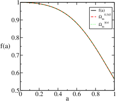
and for a CDM model . The behavior of the growth index for a model is shown in Fig. (1). We can see that there is almost no difference in behavior between the curves obtained with the approximation (17). Because of the dependence of on the dark energy parameters, the derivatives of the growth factor are given by:
| (18) | |||||
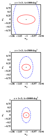
In this case the new set of parameters is and we assume as fiducial model . The factor , in this case, depends only on the dark energy parameters and ; this means the only non-vanishing derivatives are and . In Fig. (2) the confidence regions are shown for different combination of redshift and area. Instead of we use the pivot parameters (projection of on the pivot point, defined as the value of for which the uncertainty in is smallest).


| % | ||||||
| % | ||||||
| % | ||||||
| % | ||||||
IV.2 Case 2
We want now to put constraints on as a free parameter. We assume here and again as fiducial value. The new set of parameters is therefore . The derivatives with respect to the first three parameters are given by the eq. (18). The derivative for the growth factor with respect to is:
| (19) | |||||
| % | ||||||
| % | ||||||
| % | ||||||
| % | ||||||
V Results and Conclusions
The main aim of this work is to give marginalized constraints on the dark energy parameters () and most importantly on the growth factor itself, for several combinations of surveys, redshift errors and area. Following SE and Amendola, Quercellini, Giallongo (2004) we consider several binned surveys with average redshift depth around and plus a SDSS-like survey at , as detailed in Table 3. More details can be found in AQG. We consider both spectroscopic surveys ( ) and photometric surveys () and three areas ( deg2). These features are well within the range of proposed experiments like JDEM and DUNE (Crotts at al. 2005; Réfrégier et al. 2006; see also DETF Report Albrecht et al. 2006)
We first consider Case I, in which the growth factor is not an independent quantity but is a function of . The two-dimensional regions of confidence are shown in Fig (2) and the final marginalized errors are summarized in Tab. (4). The errors on reduce from 0.036 to 0.012 for the spectroscopic case for surveys that extend from 1000 to 10000 deg2 and from 0.054 to 0.018 in the photometric case.
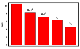
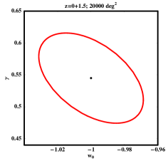
Then we consider Case II, in which is a free constant as in eq. (1). In Fig. (4) we show the confidence regions for . The errors are given in Tab. (5) . We see that the errors on reduce from 0.099 to 0.05 for spectroscopic surveys and from 0.301 to 0.114 in the photo- case. These errors are way too large to produce an independent constraint on (in fact one has approximately near ) but, beside being a general test of consistency for the cosmological model, they would certainly give interesting constraints on models that predict growths different from standard, like modified gravity models (Koyama & Maartens 2005; Maartens 2006; Amendola, Charmousis & Davis 2005; Amendola, Polarski, Tsujikawa 2006). In Fig. (3) we show the FOM for , for only one survey () and only one combination of redshift (), first when all the other parameters are fixed and then successively marginalizing over the parameter indicated and over all those on the left (eg the third column represents the marginalization over , ).
We can compare our results to those obtained recently by Huterer and Linder (2006). Using a combination of weak lensing, SNIa and CMB methods, they predict for future experiments. With large-scale tomographic weak lensing alone, Amendola, Kunz, and Sapone (2007) predict at confidence level. These values are comparable to those obtained here with the BAO method and considering a spectroscopic survey of 5000, .
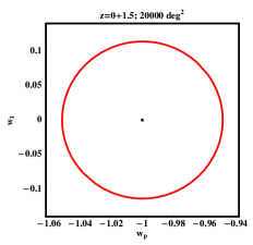
We notice that the difference on the growth index between General Relativity and an extradimensional gravity model (as DGP, where , see Linder & Cahn 2007) is ; if we compare our results shown in Tab. (5) we see that the errors on for a photometric survey are within this range, meaning that DGP model cannot be escluded. Things get slightly better if we consider spectroscopic surveys, where errors decrease with about ; however in this case we require a large survey extended from to with an area of to distinguish with sufficient confidence DGP from CDM. In Fig. (6) is shown the confidence region for for a survey extended from to and an area of (DETF case): the error on reduces to .
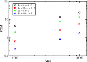
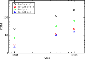
In Fig. (7) we also show the figure-of-merit (FOM) suggested by the Dark Energy Task Force report ( Albrecht et al. 2006) as a simple measure of the constraining power of an experiment. The FOM is defined as the inverse of the area that encloses the 95% confidence region and can be found simply as . In Fig. (8) we plot the FOM for and . The general trend is that the FOM for spectroscopic surveys are roughly 4-6 times higher than for similar 4% error photo- surveys. It will be interesting to compare our FOM on the plane with those obtained from other experiments. This task will be performed in future work.
Acknowledgements.
D.S. is supported by the Swiss NSF. It is a pleasure to thank Martin Kunz for interesting discussions.References
- (1) Albrecht A. et al., Dark Energy Task Force report to the Astronomy and Astrophysics Advisory Committee, DETF http://www.nsf.gov/mps/ast/detf.jsp
- (2) Amendola L., Charmousis C. & Davis S., hep-th/0506137
- (3) Amendola L., Quercellini C. & Giallongo E., MNRAS 357, 429 (2005)
- (4) Amendola L., Kunz M., &Sapone D. (2007), astro-ph/0704.2421
- (5) Amendola L. & D.Tocchini-Valentini, Phys. Rev. D 66: 043528 (2002) astro-ph/ 0111535
- (6) Amendola L., Polarski D. & Tsujikawa S., astro-ph/0603703
- (7) Astier P. et al. A&A 447, 31 (2006) astro-ph/0510447
- (8) Blake C. & Glazebrook K., Ap. J. 594, 665 (2003), astro-ph/0301632
- (9) Bennet C. et al, Ap. J. 583, 1-23, (2003), astro-ph/0301158
- (10) S. Boughn and R. Crittenden, Nature, 427, 45 (2004)
- (11) Caldwell R., A. Cooray and A. Melchiorri, astro-ph/0703375,
- (12) Copeland E., Sami M. & Tsujikawa S., hep-th/0603057
- (13) Crotts A. at al. (2005), astro-ph/0507043
- (14) Di Porto C. & Amendola L. (2007), astro-ph/0707.2686
- (15) Demianski M., Piedipalumbo E., Rubano C. & Tortora C., (2004); A&A no=041508; astro-ph/0410445
- (16) Eisenstein D. J. et al. [SDSS collaboration] Ap. J. 633, 560 (2005) astro-ph/0501171
- (17) Eisenstein D. J. & Hu W., Ap. J. 511, 5 (1999)
- (18) Eisenstein D.J. , Hu W. & Tegmark M., 1999 ApJ 518, 2
- (19) Hamilton A. J. S. & Culhane M., 1995, MNRAS (1996) 278, 73-86; astro-ph/9507021
- (20) Halverson N. W. et al., (2001) Ap.J. textbf568, 38 (2002), astro-ph/0104489
- (21) Hawkins E. et al. MNRAS 346, 78 (2003) astro-ph/0212375;
- (22) Huterer D. & Linder E. V.; astro-ph/0608681
- (23) Heavens A., T. Kitching & A. Taylor, MNARS 373, 105 (2006)
- (24) Heavens A., T. D. Kitching, L. Verde , astro-ph/0703191
- (25) Koyama K. & Maartens R., JCAP 0601 (2006) astro-ph/0511634
- (26) Ishak M., MNRAS 363, 469 (2005);
- (27) Lahav O. et al. MNRAS, 251, 128 (1991)
- (28) Lee A. T. et al., Ap.J. 561, L1 (2001) astro-ph/0104459
- (29) Linder, E. V. 2003, Phys. Rev. D 68, 083504 (2003)
- (30) Linder E.V. 2005 astro-ph/0608681
- (31) E.V. Linder and Cahn, astro-ph/0701317 (2007).
- (32) Maartens R., astro-ph/0602415
- (33) McDonald et al. Ap.J. 635, 761 (2005)
- (34) Netterfield C. B. et al., (2001) Ap.J. 571, 604 (2002) astro-ph/0104460
- (35) Nunes N. J. & Mota D. F. (2004) MNRAS 368, 751 (2006); astro-ph/0409481
- (36) Percival W. A&A 3637 (2005), astro-ph/058156
- (37) Perlmutter S. et al. (1999) Ap.J., 517, 565
- (38) Réfrégier A. et al. (2006); Procs. of symposium “Astronomical Telescopes and Instrumentation”; astro-ph/0610062
- (39) Riess et al. (2004) astro-ph/0402512
- (40) Riess A. G. et al. A.J., 116, 1009 (1998)
- (41) Scoccimarro, R. 2004, Phys. Rev. D 70 (2004) 083007, astro-ph/0407214
- (42) Seo H. J. & Eisenstein D. J., Ap. J. 598, 720 (2003), astro-ph/0307460
- (43) Spergel D.N. et al. [WMAP collaboration], Ap.J. submitted (2006)
- (44) Taylor A. et al. MNRAS 374, 1377 (2007);
- (45) Tegmark M. 1997, Phys. Rev. Lett. 79 3806
- (46) Tegmark et al,. (2004) PRD 69, 103501 astro-ph/0310723
- (47) Tonry J.T. et al. 2003, Ap.J. 594, 1
- (48) Verde L. et al. MNRAS 335, 432 (2002) astro-ph/0112161
- (49) Wang L., P. J. Steinhardt, Ap.J. 508, 483,1998.
- (50) Zaurobi S. & Hoffman Y., astro-ph/9311013
- (51) Zhang P. et al. arXiv:0704.1932 [astro-ph]