Enumeration formulas for Young tableaux in a diagonal strip

Yuliy Baryshnikov Mathematical and Algorithmic Sciences, Bell Laboratories, Murray Hill, NJ, USA. email: ymb@research.bell-labs.com .    Dan Romik Einstein Institute of Mathematics, The Hebrew University, Jerusalem, Israel. email: romik@math.huji.ac.il .
Abstract

We derive combinatorial identities, involving the Bernoulli and Euler numbers, for the numbers of standard Young tableaux of certain skew shapes. This generalizes the classical formulas of D. André on the number of up-down permutations. The analysis uses a transfer operator approach extending the method of Elkies, combined with an identity expressing the volume of a certain polytope in terms of a Schur function.

Key words: Young tableau, skew Young diagram, enumeration, up-down permutations, Schur functions, Markovian polytope, transfer operator, exactly solvable model.


MSC 2000 subject classifications: 05E10, 05A15, 05A19, 82B23

1 Introduction

1.1 Up-down permutations and the Euler, tangent and Bernoulli numbers

An up-down permutation on n𝑛n elements is a permutation σSn𝜎subscript𝑆𝑛\sigma\in S_{n} satisfying

σ(1)<σ(2)>σ(3)<σ(4)>.𝜎1expectation𝜎2𝜎3expectation𝜎4\sigma(1)<\sigma(2)>\sigma(3)<\sigma(4)>\cdots.

Up-down permutations, also known as zig-zag- or alternating permutations, were first studied in 1879 by D. André [2, 3]. He showed that if Ansubscript𝐴𝑛A_{n} denotes the number of n𝑛n-element up-down permutations, then the exponential generating function

fup-down(x)=n=0Anxnn!subscript𝑓up-down𝑥superscriptsubscript𝑛0subscript𝐴𝑛superscript𝑥𝑛𝑛f_{\text{up-down}}(x)=\sum_{n=0}^{\infty}\frac{A_{n}x^{n}}{n!}

is given by

fup-down(x)=tanx+secx.subscript𝑓up-down𝑥𝑥𝑥f_{\text{up-down}}(x)=\tan x+\sec x. (1)

In other words, tanx𝑥\tan x is the exponential g.f. of the even-indexed Ansubscript𝐴𝑛A_{n}’s, and secx𝑥\sec x is the e.g.f. of the odd-indexed Ansubscript𝐴𝑛A_{n}’s. This relates the sequence (An)subscript𝐴𝑛(A_{n}) to the Euler numbers Ensubscript𝐸𝑛E_{n} and tangent numbers Tnsubscript𝑇𝑛T_{n}, traditionally defined by the Taylor series expansions

secx𝑥\displaystyle\sec x =\displaystyle= n=0(1)nE2nx2n(2n)!,superscriptsubscript𝑛0superscript1𝑛subscript𝐸2𝑛superscript𝑥2𝑛2𝑛\displaystyle\sum_{n=0}^{\infty}\frac{(-1)^{n}E_{2n}x^{2n}}{(2n)!},
tanx𝑥\displaystyle\tan x =\displaystyle= n=1Tnx2n1(2n1)!.superscriptsubscript𝑛1subscript𝑇𝑛superscript𝑥2𝑛12𝑛1\displaystyle\sum_{n=1}^{\infty}\frac{T_{n}x^{2n-1}}{(2n-1)!}.

In terms of these numbers, we have that

A2n=(1)nE2n,A2n1=Tn.formulae-sequencesubscript𝐴2𝑛superscript1𝑛subscript𝐸2𝑛subscript𝐴2𝑛1subscript𝑇𝑛A_{2n}=(-1)^{n}E_{2n},\qquad A_{2n-1}=T_{n}. (2)

Recall also that the tangent numbers are related to the Bernoulli numbers Bnsubscript𝐵𝑛B_{n}, defined by the Taylor series expansion

xex1=n=0Bnxnn!,𝑥superscript𝑒𝑥1superscriptsubscript𝑛0subscript𝐵𝑛superscript𝑥𝑛𝑛\frac{x}{e^{x}-1}=\sum_{n=0}^{\infty}\frac{B_{n}x^{n}}{n!},

via the relation

Tn=(1)n14n(4n1)2nB2n.subscript𝑇𝑛superscript1𝑛1superscript4𝑛superscript4𝑛12𝑛subscript𝐵2𝑛T_{n}=\frac{(-1)^{n-1}4^{n}(4^{n}-1)}{2n}B_{2n}. (3)

For an amusing appearance of Euler and tangent numbers unrelated to up-down permutations, see [9]. The notation En,Tnsubscript𝐸𝑛subscript𝑇𝑛E_{n},T_{n} and Bnsubscript𝐵𝑛B_{n} will be used throughout the paper, always signifying the Euler, tangent and Bernoulli numbers, respectively, and Ansubscript𝐴𝑛A_{n} will be used throughout to denote the number of up-down permutations of order n𝑛n, given by (2).

1.2 Standard Young tableaux

It is well-known ([13, Ex. 23, p. 68], [15, Ex. 7.64.a, p. 469–470, 520]), that up-down permutations can be thought of as a special case of a standard Young tableau. Recall that an integer partition is a sequence λ=(λ1,λ2,,λk)𝜆subscript𝜆1subscript𝜆2subscript𝜆𝑘\lambda=(\lambda_{1},\lambda_{2},\ldots,\lambda_{k}), where λ1λ2>>λk>0subscript𝜆1subscript𝜆2subscript𝜆𝑘0\lambda_{1}\geq\lambda_{2}>\ldots>\lambda_{k}>0 are integers. We identify such a partition λ𝜆\lambda with its Young diagram, which is the set {(i,j)2:1ik, 1jλi}conditional-set𝑖𝑗superscript2formulae-sequence1𝑖𝑘1𝑗subscript𝜆𝑖\{(i,j)\in\mathbb{N}^{2}:1\leq i\leq k,\ 1\leq j\leq\lambda_{i}\}, graphically depicted as a set of squares, (also called cells or boxes) in the plane, traditionally in the “English notation” whereby y𝑦y-coordinate increases from top to bottom (similarly to matrix row indices in linear algebra). A skew Young diagram is the difference λμ𝜆𝜇\lambda\setminus\mu of two Young diagrams where μλ𝜇𝜆\mu\subset\lambda. If λμ𝜆𝜇\lambda\setminus\mu is a skew Young diagram, a standard Young tableau (SYT) of shape λμ𝜆𝜇\lambda\setminus\mu is a filling of the boxes of λμ𝜆𝜇\lambda\setminus\mu with the integers 1,2,,|λμ|12𝜆𝜇1,2,\ldots,|\lambda\setminus\mu| that is increasing along rows and columns. See Figure 1 for an example.

555111111666888111444121212141414333101010131313222777999
(a) (b)
Figure 1: (a) The skew Young diagram (5,5,5,3,2)(2,2,1,1,0)5553222110(5,5,5,3,2)\setminus(2,2,1,1,0). (b) A standard Young tableau (SYT).

Up-down permutations on n𝑛n elements are in simple bijection with SYT’s of shape

(m+1,m,m1,m2,,3,2)(m1,m2,,1,0)𝑚1𝑚𝑚1𝑚232𝑚1𝑚210(m+1,m,m-1,m-2,\ldots,3,2)\setminus(m-1,m-2,\ldots,1,0)

when n=2m𝑛2𝑚n=2m is even, or

(m,m,m1,m2,,3,2)(m1,m2,,1,0)𝑚𝑚𝑚1𝑚232𝑚1𝑚210(m,m,m-1,m-2,\ldots,3,2)\setminus(m-1,m-2,\ldots,1,0)

when n=2m1𝑛2𝑚1n=2m-1 is odd. The bijection converts such an SYT into an up-down permutation by reading the values starting from the bottom-left box and going alternately to the right and up. See Figure 2.

555222444333111888999101010777666 ​​​​​​​​​​​​​​​​​​​​​​​​​​​​​​​​​​​​​​ σ=(1234567891058294103716)𝜎1234567891058294103716\sigma=\left(\begin{array}[]{cccccccccc}1&2&3&4&5&6&7&8&9&10\\ 5&8&2&9&4&10&3&7&1&6\end{array}\right)


Figure 2: A standard Young tableau of shape (5,5,4,3,2,1)(4,3,2,1,0,0)554321432100(5,5,4,3,2,1)\setminus(4,3,2,1,0,0) and the associated up-down permutation.

Our main interest will be in enumerating SYT’s of shapes in a special family. For a skew Young diagram D=λμ𝐷𝜆𝜇D=\lambda\setminus\mu, denote by f(D)𝑓𝐷f(D) the number of SYT’s of shape D𝐷D (this is frequently denoted by fλμsuperscript𝑓𝜆𝜇f^{\lambda\setminus\mu}, but the current notation will be more convenient for our purposes). Recall the formula of Aitken [1] (later rediscovered by Feit [12]; see also [15, Corollary 7.16.3, p. 344], [13, Ex. 19, p. 67, 609]) for f(D)𝑓𝐷f(D):

f(D)=|λμ|!det(1(λiiμj+j)!)i,j.𝑓𝐷𝜆𝜇subscript1subscript𝜆𝑖𝑖subscript𝜇𝑗𝑗𝑖𝑗f(D)=|\lambda\setminus\mu|!\det\Big{(}\frac{1}{(\lambda_{i}-i-\mu_{j}+j)!}\Big{)}_{i,j}. (4)

Using (4) can become difficult when the diagrams λ𝜆\lambda and μ𝜇\mu are large (even when their difference is small!), as the order of the determinant is equal to the number of parts in λ𝜆\lambda. As we shall see below, in certain cases one can give more concise formulas that also relate the numbers of SYT’s of different shapes to each other, and notably to the “zig-zag” numbers (An)n0subscriptsubscript𝐴𝑛𝑛0(A_{n})_{n\geq 0}.

1.3 Standard Young tableaux in a strip

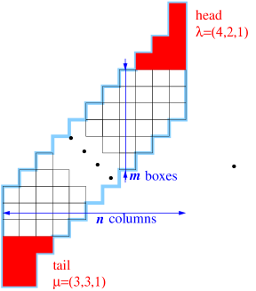
The standard Young tableaux that we will consider will be of the following general shape, which we call an m𝑚m-strip (diagonal) diagram.

Refer to caption
Figure 3: An m𝑚m-strip diagram. The head and tail rotated Young diagrams are read off in columns.

The body of the diagram consists of n𝑛n columns of m𝑚m boxes each. The head and the tail are Young diagrams that are rotated and connected to the body by leaning against the sides of the body, as shown in the figure. We will usually think of m𝑚m as fixed and n𝑛n growing, which is why we use the term m𝑚m-strip.

Our main result, Theorem 4 below, is a new formula for enumerating m𝑚m-strip tableaux (that is, SYT’s whose shape is an m𝑚m-strip diagram) in terms of the zig-zag numbers (An)n0subscriptsubscript𝐴𝑛𝑛0(A_{n})_{n\geq 0}. To introduce this formula, we start with some explicit formulas for small values of m𝑚m, and then present the general formula that contains all these formulas as special cases.

Theorem 1 (333-strip tableaux).
f([Uncaptioned image])𝑓[Uncaptioned image]\displaystyle f\left(\raisebox{-13.3472pt}{\includegraphics[width=39.83368pt]{strip_3_0_0.eps}}\right) =\displaystyle= (3n2)!Tn(2n1)!22n2,3𝑛2subscript𝑇𝑛2𝑛1superscript22𝑛2\displaystyle\frac{(3n-2)!T_{n}}{(2n-1)!2^{2n-2}}, (5)
f([Uncaptioned image])𝑓[Uncaptioned image]\displaystyle f\left(\raisebox{-14.63881pt}{\includegraphics[width=39.83368pt]{strip_3_0_1.eps}}\right) =\displaystyle= (3n1)!Tn(2n1)!22n1,3𝑛1subscript𝑇𝑛2𝑛1superscript22𝑛1\displaystyle\frac{(3n-1)!T_{n}}{(2n-1)!2^{2n-1}}, (6)
f([Uncaptioned image])𝑓[Uncaptioned image]\displaystyle f\left(\raisebox{-15.93048pt}{\includegraphics[width=39.83368pt]{strip_3_1_1.eps}}\right) =\displaystyle= (3n)!(22n11)Tn(2n1)!22n1(22n1).3𝑛superscript22𝑛11subscript𝑇𝑛2𝑛1superscript22𝑛1superscript22𝑛1\displaystyle\frac{(3n)!(2^{2n-1}-1)T_{n}}{(2n-1)!2^{2n-1}(2^{2n}-1)}. (7)
Theorem 2 (444-strip tableaux).
f([Uncaptioned image])𝑓[Uncaptioned image]\displaystyle f\left(\raisebox{-15.93048pt}{\includegraphics[width=39.83368pt]{strip_4_0_0.eps}}\right) =\displaystyle\!\!\!= (4n2)!(Tn2((2n1)!)2E2n2E2n(2n2)!(2n)!),4𝑛2superscriptsubscript𝑇𝑛2superscript2𝑛12subscript𝐸2𝑛2subscript𝐸2𝑛2𝑛22𝑛\displaystyle\!\!(4n-2)!\left(\frac{T_{n}^{2}}{((2n-1)!)^{2}}-\frac{-E_{2n-2}E_{2n}}{(2n-2)!(2n)!}\right), (8)
f([Uncaptioned image])𝑓[Uncaptioned image]\displaystyle f\left(\raisebox{-16.79158pt}{\includegraphics[width=39.83368pt]{strip_4_1_1.eps}}\right) =\displaystyle\!\!\!\!= (4n)!(E2n2((2n)!)2E2n2E2n+2(2n2)!(2n+2)!).4𝑛superscriptsubscript𝐸2𝑛2superscript2𝑛2subscript𝐸2𝑛2subscript𝐸2𝑛22𝑛22𝑛2\displaystyle\!\!(4n)!\left(\frac{E_{2n}^{2}}{((2n)!)^{2}}-\frac{E_{2n-2}E_{2n+2}}{(2n-2)!(2n+2)!}\right). (9)
Theorem 3 (555-strip tableaux).
f([Uncaptioned image])𝑓[Uncaptioned image]\displaystyle f\left(\raisebox{-17.22217pt}{\includegraphics[width=45.52458pt]{strip_5_0_0.eps}}\right) =\displaystyle= (5n6)!Tn12((2n3)!)224n6(22n21).5𝑛6superscriptsubscript𝑇𝑛12superscript2𝑛32superscript24𝑛6superscript22𝑛21\displaystyle\frac{(5n-6)!T_{n-1}^{2}}{((2n-3)!)^{2}2^{4n-6}(2^{2n-2}-1)}.

The formulas in Theorems 1, 2, 3 are special cases of an infinite family of formulas. To formulate them, we introduce some notation. Let A¯n=An/n!subscript¯𝐴𝑛subscript𝐴𝑛𝑛\bar{A}_{n}=A_{n}/n! (the volume of the n𝑛n-th up-down polytope, see Section 2). Let

A~n=A¯n2n+11,A^n=(2n1)A¯n2n(2n+11).formulae-sequencesubscript~𝐴𝑛subscript¯𝐴𝑛superscript2𝑛11subscript^𝐴𝑛superscript2𝑛1subscript¯𝐴𝑛superscript2𝑛superscript2𝑛11\tilde{A}_{n}=\frac{\bar{A}_{n}}{2^{n+1}-1},\qquad\hat{A}_{n}=\frac{(2^{n}-1)\bar{A}_{n}}{2^{n}(2^{n+1}-1)}.

For nonnegative integers p,q,N𝑝𝑞𝑁p,q,N, denote

XN(p,q)subscript𝑋𝑁𝑝𝑞\displaystyle X_{N}(p,q) =\displaystyle= i=0p/2j=0q/2(1)i+jA¯N+2i+2j+1(p2i)!(q2j)!superscriptsubscript𝑖0𝑝2superscriptsubscript𝑗0𝑞2superscript1𝑖𝑗subscript¯𝐴𝑁2𝑖2𝑗1𝑝2𝑖𝑞2𝑗\displaystyle\sum_{i=0}^{\lfloor p/2\rfloor}\sum_{j=0}^{\lfloor q/2\rfloor}\frac{(-1)^{i+j}\bar{A}_{N+2i+2j+1}}{(p-2i)!(q-2j)!}
+(1)p+12j=0q/2(1)jA¯N+p+2j+1(q2j)!1[p odd]superscript1𝑝12superscriptsubscript𝑗0𝑞2superscript1𝑗subscript¯𝐴𝑁𝑝2𝑗1𝑞2𝑗subscript1delimited-[]𝑝 odd\displaystyle+(-1)^{\frac{p+1}{2}}\sum_{j=0}^{\lfloor q/2\rfloor}\frac{(-1)^{j}\bar{A}_{N+p+2j+1}}{(q-2j)!}1_{[p\text{ odd}]}
+(1)q+12i=0p/2(1)iA¯N+q+2i+1(p2i)!1[q odd]superscript1𝑞12superscriptsubscript𝑖0𝑝2superscript1𝑖subscript¯𝐴𝑁𝑞2𝑖1𝑝2𝑖subscript1delimited-[]𝑞 odd\displaystyle+(-1)^{\frac{q+1}{2}}\sum_{i=0}^{\lfloor p/2\rfloor}\frac{(-1)^{i}\bar{A}_{N+q+2i+1}}{(p-2i)!}1_{[q\text{ odd}]}
+(1)p+q2+1A¯N+p+q+11[p,q odd],superscript1𝑝𝑞21subscript¯𝐴𝑁𝑝𝑞1subscript1𝑝𝑞 odd\displaystyle+(-1)^{\frac{p+q}{2}+1}\bar{A}_{N+p+q+1}1_{[p,q\text{ odd}]},
YN(p,q)subscript𝑌𝑁𝑝𝑞\displaystyle Y_{N}(p,q) =\displaystyle= i=0p/2j=0q/2(1)i+jA^N+2i+2j+1(p2i)!(q2j)!superscriptsubscript𝑖0𝑝2superscriptsubscript𝑗0𝑞2superscript1𝑖𝑗subscript^𝐴𝑁2𝑖2𝑗1𝑝2𝑖𝑞2𝑗\displaystyle\sum_{i=0}^{\lfloor p/2\rfloor}\sum_{j=0}^{\lfloor q/2\rfloor}\frac{(-1)^{i+j}\hat{A}_{N+2i+2j+1}}{(p-2i)!(q-2j)!}
+(1)p2j=0q/2(1)jA~N+p+2j+1(q2j)!1[p even]superscript1𝑝2superscriptsubscript𝑗0𝑞2superscript1𝑗subscript~𝐴𝑁𝑝2𝑗1𝑞2𝑗subscript1delimited-[]𝑝 even\displaystyle+(-1)^{\frac{p}{2}}\sum_{j=0}^{\lfloor q/2\rfloor}\frac{(-1)^{j}\tilde{A}_{N+p+2j+1}}{(q-2j)!}1_{[p\text{ even}]}
+(1)q2i=0p/2(1)iA~N+q+2i+1(p2i)!1[q even]superscript1𝑞2superscriptsubscript𝑖0𝑝2superscript1𝑖subscript~𝐴𝑁𝑞2𝑖1𝑝2𝑖subscript1delimited-[]𝑞 even\displaystyle+(-1)^{\frac{q}{2}}\sum_{i=0}^{\lfloor p/2\rfloor}\frac{(-1)^{i}\tilde{A}_{N+q+2i+1}}{(p-2i)!}1_{[q\text{ even}]}
+(1)p+q2A^N+p+q+11[p,q even],superscript1𝑝𝑞2subscript^𝐴𝑁𝑝𝑞1subscript1𝑝𝑞 even\displaystyle+(-1)^{\frac{p+q}{2}}\hat{A}_{N+p+q+1}1_{[p,q\text{ even}]},

(here 1[x]subscript1delimited-[]𝑥1_{[x]} is 1 if x𝑥x is true, 0 otherwise). Then we have

Theorem 4.

Let D𝐷D be an m𝑚m-strip diagram as in Figure 3. Denote the head Young diagram by (λ1,λ2,,λk)subscript𝜆1subscript𝜆2subscript𝜆𝑘(\lambda_{1},\lambda_{2},\ldots,\lambda_{k}) and the tail Young diagram by (μ1,μ2,,μk)subscript𝜇1subscript𝜇2subscript𝜇𝑘(\mu_{1},\mu_{2},\ldots,\mu_{k}) (where k=m/2𝑘𝑚2k=\lfloor m/2\rfloor). Define the associated numbers Li=λi+kisubscript𝐿𝑖subscript𝜆𝑖𝑘𝑖L_{i}=\lambda_{i}+k-i and Mi=μi+kisubscript𝑀𝑖subscript𝜇𝑖𝑘𝑖M_{i}=\mu_{i}+k-i, i=1,,k𝑖1𝑘i=1,\ldots,k. If the diagram has a total of n𝑛n columns, then the number of SYT’s of shape D𝐷D is given by

f(D)=(1)(k2)|D|!det(X2nm+1(Li,Mj))i,j=1,,k𝑓𝐷superscript1binomial𝑘2𝐷𝑑𝑒𝑡subscriptsubscript𝑋2𝑛𝑚1subscript𝐿𝑖subscript𝑀𝑗formulae-sequence𝑖𝑗1𝑘f(D)=(-1)^{\binom{k}{2}}|D|!\ det\bigg{(}X_{2n-m+1}(L_{i},M_{j})\bigg{)}_{i,j=1,\ldots,k} (10)

if m𝑚m is even, or by

f(D)=(1)(k2)|D|!det(Y2nm+1(Li,Mj))i,j=1,,k𝑓𝐷superscript1binomial𝑘2𝐷𝑑𝑒𝑡subscriptsubscript𝑌2𝑛𝑚1subscript𝐿𝑖subscript𝑀𝑗formulae-sequence𝑖𝑗1𝑘f(D)=(-1)^{\binom{k}{2}}|D|!\ det\bigg{(}Y_{2n-m+1}(L_{i},M_{j})\bigg{)}_{i,j=1,\ldots,k} (11)

if m𝑚m is odd.

Note that XN(p,q)subscript𝑋𝑁𝑝𝑞X_{N}(p,q) and YN(p,q)subscript𝑌𝑁𝑝𝑞Y_{N}(p,q) are linear combinations of the zig-zag numbers AN+1,AN+2,,AN+p+q+1subscript𝐴𝑁1subscript𝐴𝑁2subscript𝐴𝑁𝑝𝑞1A_{N+1},A_{N+2},\ldots,A_{N+p+q+1}. Thus, the theorem represents f(D)𝑓𝐷f(D) for an m𝑚m-strip diagram as a polynomial in the numbers Ansubscript𝐴𝑛A_{n}, whose complexity depends on the thickness m𝑚m of the strip but not on the number of columns n𝑛n. For example, for the diagram D𝐷D in equation (9) we have (λ1,λ2)=(μ1,μ2)=(1,0)subscript𝜆1subscript𝜆2subscript𝜇1subscript𝜇210(\lambda_{1},\lambda_{2})=(\mu_{1},\mu_{2})=(1,0), so we get

f(D)𝑓𝐷\displaystyle f(D) =\displaystyle= (4n)!det(X2n3(0,0)X2n3(0,2)X2n3(2,0)X2n3(2,2))4𝑛subscript𝑋2𝑛300subscript𝑋2𝑛302subscript𝑋2𝑛320subscript𝑋2𝑛322\displaystyle-(4n)!\det\left(\begin{array}[]{ll}X_{2n-3}(0,0)&X_{2n-3}(0,2)\\ X_{2n-3}(2,0)&X_{2n-3}(2,2)\end{array}\right)
=\displaystyle= (4n)!det(A¯2n212A¯2n2A¯2n12A¯2n2A¯2n14A¯2n2A¯2n+A¯2n+2),4𝑛subscript¯𝐴2𝑛212subscript¯𝐴2𝑛2subscript¯𝐴2𝑛12subscript¯𝐴2𝑛2subscript¯𝐴2𝑛14subscript¯𝐴2𝑛2subscript¯𝐴2𝑛subscript¯𝐴2𝑛2\displaystyle-(4n)!\det\left(\begin{array}[]{ll}\bar{A}_{2n-2}&\frac{1}{2}\bar{A}_{2n-2}-\bar{A}_{2n}\\ \frac{1}{2}\bar{A}_{2n-2}-\bar{A}_{2n}&\frac{1}{4}\bar{A}_{2n-2}-\bar{A}_{2n}+\bar{A}_{2n+2}\end{array}\right),

which simplifies to give (9). By comparison, trying to use (4) to compute f(D)𝑓𝐷f(D) would result in a daunting-looking determinant of order n+3𝑛3n+3, whose relation to the analogous determinants for the Ansubscript𝐴𝑛A_{n}’s is unclear.

The following theorem gives a direct combinatorial meaning to XN(p,q)subscript𝑋𝑁𝑝𝑞X_{N}(p,q). The first part is a simple corollary to Theorem 4, and the second part does not follow from Theorem 4 but can be proved using the same techniques – see Section 8.

Theorem 5.

For a permutation σSn𝜎subscript𝑆𝑛\sigma\in S_{n} and 1in11𝑖𝑛11\leq i\leq n-1, we say that σ𝜎\sigma has a descent at i𝑖i if σ(i)>σ(i+1)𝜎𝑖𝜎𝑖1\sigma(i)>\sigma(i+1). For integers n,p,q0𝑛𝑝𝑞0n,p,q\geq 0, denote by αnsubscript𝛼𝑛\alpha_{n} the number of permutations in S2n+p+qsubscript𝑆2𝑛𝑝𝑞S_{2n+p+q} whose set of descents is equal to

{1,2,3,,p,p+1,p+3,p+5,,p+2n3,p+2n1,p+2n,p+2n+1,p+2n+q1}.123𝑝𝑝1𝑝3𝑝5𝑝2𝑛3𝑝2𝑛1𝑝2𝑛𝑝2𝑛1𝑝2𝑛𝑞1\{1,2,3,\ldots,p,p+1,p+3,p+5,\ldots,p+2n-3,p+2n-1,\\ p+2n,p+2n+1\ldots,p+2n+q-1\}.

Denote by βnsubscript𝛽𝑛\beta_{n} the number of permutations in S2n+p+qsubscript𝑆2𝑛𝑝𝑞S_{2n+p+q} whose descent set is equal to

{1,2,3,,p,p+1,p+3,p+5,,p+2n3,p+2n1}123𝑝𝑝1𝑝3𝑝5𝑝2𝑛3𝑝2𝑛1\{1,2,3,\ldots,p,p+1,p+3,p+5,\ldots,p+2n-3,p+2n-1\}

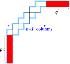
(equivalently, αnsubscript𝛼𝑛\alpha_{n} and βnsubscript𝛽𝑛\beta_{n} count SYT’s of the shapes shown in Figure 4 below). Then we have

αnsubscript𝛼𝑛\displaystyle\alpha_{n} =\displaystyle= (2n+p+q)!X2n1(p,q),2𝑛𝑝𝑞subscript𝑋2𝑛1𝑝𝑞\displaystyle(2n+p+q)!X_{2n-1}(p,q), (14)
βnsubscript𝛽𝑛\displaystyle\beta_{n} =\displaystyle= (2n+1+p+q)!X2n(p,q).2𝑛1𝑝𝑞subscript𝑋2𝑛𝑝𝑞\displaystyle(2n+1+p+q)!X_{2n}(p,q). (15)

Similarly, one can also give a combinatorial meaning to YN(p,q)subscript𝑌𝑁𝑝𝑞Y_{N}(p,q) in terms of the number of SYT’s for certain 333-strip diagrams. We leave the precise formulation of this statement to the reader, as an exercise in implementing the techniques of Section 8.
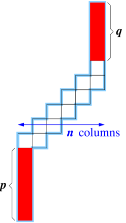
Refer to caption Refer to caption
Figure 4: The shapes whose standard Young tableaux are enumerated by αnsubscript𝛼𝑛\alpha_{n} and βnsubscript𝛽𝑛\beta_{n}, respectively.

In the next sections we develop the tools that will be used to prove the theorems above. The idea is to use transfer operators. This generalizes the transfer operator approach to up-down permutations introduced by Elkies [10]. Another tool is a geometric-combinatorial identity that expresses the volume of a certain polytope in terms of a Schur symmetric function, and can be thought of as a continuous analogue of a known result on the enumeration of certain shifted Young tableaux. This identity, Proposition 12, is the subject of Section 7.

The understanding of m𝑚m-strip tableaux that we gain using our analysis of the transfer operators gives more, and is perhaps more important, than just the proof of the formulas given above. In fact, more general formulas could be derived, and even more results such as an understanding of random m𝑚m-strip tableaux of given shape. Thus, we have the following theorem.

Theorem 6.

The m𝑚m-strip tableaux model is an exactly solvable model in the statistical mechanics sense (see Baxter [7]). That is, the transfer operators can be explicitly diagonalized.

For more details, see Theorems 10, 11 and comment 1 in Section 9.

To conclude this introduction, we note that the m𝑚m-strip tableaux model is related to the bead model studied by Boutillier [8]: The Gibbs measures he constructs seem to describe the limiting distribution of uniform random elements of the order polytope (see Section 4 for the definition) associated with an m𝑚m-strip diagram. The m𝑚m-strip tableaux model is also related to the square ice model from statistical physics (see [7, Chapter 8]), and our explicit diagonalization of the transfer operators can be thought of as a degenerate case of the so-called Bethe ansatz used in the solution of that model.

1.4 Acknowledgements

Theorem 1, from which this project evolved, was first discovered and proved when the second-named author was visiting Microsoft Research in 2004, in collaboration with Henry Cohn, Assaf Naor and Yuval Peres. We are also grateful to George Andrews, Omer Angel, Cedric Boutillier, Ehud Friedgut, Ander Holroyd, Rick Kenyon, Christian Krattenthaler, Andrei Okounkov, Igor Pak, Andrea Sportiello, Bálint Virág and Doron Zeilberger for helpful discussions.

2 The transfer operator method of Elkies

Noam Elkies [10] proposed the following approach to proving (1). Define the n𝑛n-th up-down polytope by

Pn={(x1,,xn)[0,1]n:x1x2x3x4}.subscript𝑃𝑛conditional-setsubscript𝑥1subscript𝑥𝑛superscript01𝑛subscript𝑥1subscript𝑥2subscript𝑥3subscript𝑥4P_{n}=\{(x_{1},\ldots,x_{n})\in[0,1]^{n}\ :\ x_{1}\leq x_{2}\geq x_{3}\leq x_{4}\geq\ldots\ \}.

Computing vol(Pn)volsubscript𝑃𝑛\mathrm{vol}(P_{n}), the volume of Pnsubscript𝑃𝑛P_{n}, in two ways, one first observes that this is simply related to the number Ansubscript𝐴𝑛A_{n} of up-down permutations by

vol(Pn)=Ann!.volsubscript𝑃𝑛subscript𝐴𝑛𝑛\mathrm{vol}(P_{n})=\frac{A_{n}}{n!}.

This is because (in probabilistic language) n𝑛n independently drawn uniform random variables in [0,1]01[0,1] will be in Pnsubscript𝑃𝑛P_{n} with probability An/n!subscript𝐴𝑛𝑛A_{n}/n!, since for each up-down permutation σ𝜎\sigma the probability is 1/n!1𝑛1/n! that the random variables will have order structure σ𝜎\sigma, and these events have measure 0 pairwise intersections.

On the other hand, by computing the volume as an iterated integral, namely

vol(Pn)=01𝑑x1x11𝑑x20x2𝑑x3x31𝑑x4,volsubscript𝑃𝑛superscriptsubscript01differential-dsubscript𝑥1superscriptsubscriptsubscript𝑥11differential-dsubscript𝑥2superscriptsubscript0subscript𝑥2differential-dsubscript𝑥3superscriptsubscriptsubscript𝑥31differential-dsubscript𝑥4\mathrm{vol}(P_{n})=\int_{0}^{1}dx_{1}\int_{x_{1}}^{1}dx_{2}\int_{0}^{x_{2}}dx_{3}\int_{x_{3}}^{1}dx_{4}\ldots,

upon some more simple manipulation one obtains the following convenient representation in terms of linear operators on the function space L2[0,1]subscript𝐿201L_{2}[0,1]:

vol(Pn)=Tn1(𝟏),𝟏,volsubscript𝑃𝑛superscript𝑇𝑛111\mathrm{vol}(P_{n})=\Big{\langle}T^{n-1}(\mathbf{1}),\mathbf{1}\Big{\rangle}, (16)

where 𝟏1\mathbf{1} is the constant function 111, T:L2[0,1]L2[0,1]:𝑇subscript𝐿201subscript𝐿201T:L_{2}[0,1]\to L_{2}[0,1] is the self-adjoint operator given by

(Tf)(x)=01xf(y)𝑑y,𝑇𝑓𝑥superscriptsubscript01𝑥𝑓𝑦differential-d𝑦(Tf)(x)=\int_{0}^{1-x}f(y)dy, (17)

and ,\langle\cdot,\cdot\rangle is the usual scalar product on L2[0,1]subscript𝐿201L_{2}[0,1]. The operator T𝑇T is called the transfer operator 111This operator, or rather its discrete version, was applied to up-down permutations by V. Arnold, see [5] and [14].. Transfer operators are commonly used in combinatorics and statistical mechanics (where they are sometimes called transfer matrices) and in the theory of dynamical systems. In this case, having obtained the representation (16), all that is left to do is to find the orthonormal basis (ϕk)k=1superscriptsubscriptsubscriptitalic-ϕ𝑘𝑘1(\phi_{k})_{k=1}^{\infty} of eigenfunctions, with respective eigenvalues λksubscript𝜆𝑘\lambda_{k}, of T𝑇T (note that T𝑇T is a self-adjoint operator), since then one gets that

An=n!vol(Pn)=n!k=1λkn1𝟏,ϕk2.subscript𝐴𝑛𝑛volsubscript𝑃𝑛𝑛superscriptsubscript𝑘1superscriptsubscript𝜆𝑘𝑛1superscript1subscriptitalic-ϕ𝑘2A_{n}=n!\mathrm{vol}(P_{n})=n!\sum_{k=1}^{\infty}\lambda_{k}^{n-1}\Big{\langle}{\bf 1},\phi_{k}\Big{\rangle}^{2}.

The eigenfunction problem for T𝑇T leads easily to the solutions

ϕk(x)=2cos((2k1)πx2),λk=(1)k12(2k1)π,k=1,2,3,formulae-sequencesubscriptitalic-ϕ𝑘𝑥22𝑘1𝜋𝑥2formulae-sequencesubscript𝜆𝑘superscript1𝑘122𝑘1𝜋𝑘123\phi_{k}(x)=\sqrt{2}\cos\left(\frac{(2k-1)\pi x}{2}\right),\quad\lambda_{k}=\frac{(-1)^{k-1}\cdot 2}{(2k-1)\pi},\quad k=1,2,3,\ldots

whereby one obtains, after some computations that we omit,

An=2n+2n!πn+1k=1(1)(k1)(n1)(2k1)n+1,subscript𝐴𝑛superscript2𝑛2𝑛superscript𝜋𝑛1superscriptsubscript𝑘1superscript1𝑘1𝑛1superscript2𝑘1𝑛1A_{n}=\frac{2^{n+2}n!}{\pi^{n+1}}\sum_{k=1}^{\infty}\frac{(-1)^{(k-1)(n-1)}}{(2k-1)^{n+1}}, (18)

a formula that is equivalent to (1).

3 Markovian polytopes

We wish to generalize the transfer operator method to the setting of m𝑚m-strip tableaux. For skew Young diagrams we can define their associated order polytope and try to apply the same idea to its volume computation. However, there is a certain property of the polytopes associated with up-down permutations that makes usage of the transfer operator method possible (after all, computing volumes of polytopes exactly is in general quite difficult). Borrowing from the language of probability theory, we call this property the Markov property.

Definition 7.

Let Pd𝑃superscript𝑑P\subset\mathbb{R}^{d} be a polytope. If there exists a partition of the coordinate set

{1,2,,d}=C1C2Ck(disjoint union),12𝑑subscript𝐶1subscript𝐶2subscript𝐶𝑘(disjoint union)\{1,2,\ldots,d\}=C_{1}\cup C_{2}\cup\ldots\cup C_{k}\quad\text{(disjoint union)},

such that for all j=2,,k1𝑗2𝑘1j=2,\ldots,k-1, any Cjsubscript𝐶𝑗C_{j}-section of P𝑃P, namely a set of the form

Px~:=P{xd:x|Cj=x~},P_{\tilde{x}}:=P\cap\{x\in\mathbb{R}^{d}\ :\ x_{|C_{j}}=\tilde{x}\},

where x~Cj~𝑥superscriptsubscript𝐶𝑗\tilde{x}\in\mathbb{R}^{C_{j}} is fixed, decomposes as a cartesian product of the form

Px~=Pjx~×Pj+x~,subscript𝑃~𝑥subscriptsuperscript𝑃~𝑥limit-from𝑗subscriptsuperscript𝑃~𝑥limit-from𝑗P_{\tilde{x}}=P^{\tilde{x}}_{j-}\times P^{\tilde{x}}_{j+}, (19)

where Pjx~C1×C2××Cj1subscriptsuperscript𝑃~𝑥limit-from𝑗superscriptsubscript𝐶1subscript𝐶2subscript𝐶𝑗1P^{\tilde{x}}_{j-}\subset\mathbb{R}^{C_{1}\times C_{2}\times\ldots\times C_{j-1}} and Pjx~Cj+1×Cj+2××Cksubscriptsuperscript𝑃~𝑥limit-from𝑗superscriptsubscript𝐶𝑗1subscript𝐶𝑗2subscript𝐶𝑘P^{\tilde{x}}_{j-}\subset\mathbb{R}^{C_{j+1}\times C_{j+2}\times\ldots\times C_{k}}, then we say that P𝑃P is Markovian with respect to the coordinate filtration (C1,C2,,Ck)subscript𝐶1subscript𝐶2subscript𝐶𝑘(C_{1},C_{2},\ldots,C_{k}). If P𝑃P has this property, for any j=1,2,,k1𝑗12𝑘1j=1,2,\ldots,k-1 define the j𝑗j-th transfer operator Tj:L2(Cj)L2(Cj+1):subscript𝑇𝑗subscript𝐿2superscriptsubscript𝐶𝑗subscript𝐿2superscriptsubscript𝐶𝑗1T_{j}:L_{2}(\mathbb{R}^{C_{j}})\to L_{2}(\mathbb{R}^{C_{j+1}}) associated with P𝑃P by

(Tj(f))(u)=RCjf(v)1{Pu,v}𝑑v,subscript𝑇𝑗𝑓𝑢subscriptsuperscript𝑅subscript𝐶𝑗𝑓𝑣subscript1subscript𝑃𝑢𝑣differential-d𝑣\big{(}T_{j}(f)\big{)}(u)=\int_{R^{C_{j}}}f(v)1_{\{P_{u,v}\neq\emptyset\}}dv,

where Pu,vsubscript𝑃𝑢𝑣P_{u,v} is the section

Pu,v={xd:x|Cj=v,x|Cj+1=u}.P_{u,v}=\Big{\{}x\in\mathbb{R}^{d}:x_{|C_{j}}=v,\ \ x_{|C_{j+1}}=u\Big{\}}.

The importance of these definitions becomes apparent in the following proposition, which shows how certain volumes can be represented as scalar products in some L2subscript𝐿2L_{2} space.

Proposition 8.

In the above notation, if uC1,vCkformulae-sequence𝑢superscriptsubscript𝐶1𝑣superscriptsubscript𝐶𝑘u\in\mathbb{R}^{C_{1}},v\in\mathbb{R}^{C_{k}}, then

vol(Pu,v)=Tk1Tk2T2T1(δu),δvL2(Ck).subscriptvolsubscript𝑃𝑢𝑣subscriptsubscript𝑇𝑘1subscript𝑇𝑘2subscript𝑇2subscript𝑇1subscript𝛿𝑢subscript𝛿𝑣subscript𝐿2superscriptsubscript𝐶𝑘\mathrm{vol}_{*}(P_{u,v})=\Big{\langle}T_{k-1}\circ T_{k-2}\circ\ldots\circ T_{2}\circ T_{1}(\delta_{u}),\delta_{v}\Big{\rangle}_{L_{2}(\mathbb{R}^{C_{k}})}. (20)

Here δu,δvsubscript𝛿𝑢subscript𝛿𝑣\delta_{u},\delta_{v} are Dirac delta functions centered around (respectively) u,v𝑢𝑣u,v in the respective distribution spaces, and volsubscriptvol\mathrm{vol}_{*} is the Lebesgue measure of appropriate dimensionality (in this case, d|Cj||Cj+1|𝑑subscript𝐶𝑗subscript𝐶𝑗1d-|C_{j}|-|C_{j+1}|). Furthermore,

vol(P)=Tk1Tk2T2T1(𝟏L2(C1)),𝟏L2(Ck)L2(Ck),vol𝑃subscriptsubscript𝑇𝑘1subscript𝑇𝑘2subscript𝑇2subscript𝑇1subscript1subscript𝐿2superscriptsubscript𝐶1subscript1subscript𝐿2superscriptsubscript𝐶𝑘subscript𝐿2superscriptsubscript𝐶𝑘\mathrm{vol}(P)=\Big{\langle}T_{k-1}\circ T_{k-2}\circ\ldots\circ T_{2}\circ T_{1}(\mathbf{1}_{L_{2}(\mathbb{R}^{C_{1}})}),\mathbf{1}_{L_{2}(\mathbb{R}^{C_{k}})}\Big{\rangle}_{L_{2}(\mathbb{R}^{C_{k}})}, (21)

where 𝟏1\mathbf{1} represents the constant function 111 in the respective L2subscript𝐿2L_{2} space.

Proof.

First, note the following trivial identity: If d1,d2,d3subscript𝑑1subscript𝑑2subscript𝑑3d_{1},d_{2},d_{3}\in\mathbb{N} and A:L2(d1)L2(d3),B:L2(d2)L2(d3):𝐴subscript𝐿2superscriptsubscript𝑑1subscript𝐿2superscriptsubscript𝑑3𝐵:subscript𝐿2superscriptsubscript𝑑2subscript𝐿2superscriptsubscript𝑑3A:L_{2}(\mathbb{R}^{d_{1}})\to L_{2}(\mathbb{R}^{d_{3}}),B:L_{2}(\mathbb{R}^{d_{2}})\to L_{2}(\mathbb{R}^{d_{3}}) are linear operators, then for any functions fL2(d1),gL2(d2)formulae-sequence𝑓subscript𝐿2superscriptsubscript𝑑1𝑔subscript𝐿2superscriptsubscript𝑑2f\in L_{2}(\mathbb{R}^{d_{1}}),g\in L_{2}(\mathbb{R}^{d_{2}}) we have

d3Af,δxBg,δx𝑑x=Af,Bg.subscriptsuperscriptsubscript𝑑3𝐴𝑓subscript𝛿𝑥𝐵𝑔subscript𝛿𝑥differential-d𝑥𝐴𝑓𝐵𝑔\int_{\mathbb{R}^{d_{3}}}\Big{\langle}Af,\delta_{x}\Big{\rangle}\Big{\langle}Bg,\delta_{x}\Big{\rangle}dx=\Big{\langle}Af,Bg\Big{\rangle}. (22)

Second, note that from the definition it follows that the set Pjx~superscriptsubscript𝑃limit-from𝑗~𝑥P_{j-}^{\tilde{x}} in (19) is, if it’s not empty, also Markovian with respect to the filtration (C1,,Cj1)subscript𝐶1subscript𝐶𝑗1(C_{1},\ldots,C_{j-1}), with the same transfer operators T1,,Tj2subscript𝑇1subscript𝑇𝑗2T_{1},\ldots,T_{j-2} as P𝑃P.

Now, equation (21) clearly follows from (20) by integrating over uC1,vCkformulae-sequence𝑢superscriptsubscript𝐶1𝑣superscriptsubscript𝐶𝑘u\in\mathbb{R}^{C_{1}},v\in\mathbb{R}^{C_{k}}. To prove (20), we use induction together with the above observations. For each xk1Ck1subscript𝑥𝑘1superscriptsubscript𝐶𝑘1x_{k-1}\in\mathbb{R}^{C_{k-1}} let Pu,xk1,vsubscript𝑃𝑢subscript𝑥𝑘1𝑣P_{u,x_{k-1},v} be the section

Pu,xk1,v={xd:x|Cj=v,x|Ck1=xk1,x|Cj+1=u}.P_{u,x_{k-1},v}=\Big{\{}x\in\mathbb{R}^{d}:x_{|C_{j}}=v,\ \ x_{|C_{k-1}}=x_{k-1},\ \ x_{|C_{j+1}}=u\Big{\}}.

Then

vol(Pu,v)volsubscript𝑃𝑢𝑣\displaystyle\mathrm{vol}(P_{u,v}) =\displaystyle= Ck1vol(Pu,xk1,v)𝑑xk1subscriptsuperscriptsubscript𝐶𝑘1volsubscript𝑃𝑢subscript𝑥𝑘1𝑣differential-dsubscript𝑥𝑘1\displaystyle\ \ \ \int_{\mathbb{R}^{C_{k-1}}}\mathrm{vol}(P_{u,x_{k-1},v})dx_{k-1}\qquad\qquad\qquad\qquad\qquad\qquad
=(Markov)superscript(Markov)\displaystyle\stackrel{{\scriptstyle\text{(Markov)}}}{{=}} Ck1vol(P(k1),uxk1)1{Pxk1,v}𝑑xk1subscriptsuperscriptsubscript𝐶𝑘1subscriptvolsuperscriptsubscript𝑃limit-from𝑘1𝑢subscript𝑥𝑘1subscript1subscript𝑃subscript𝑥𝑘1𝑣differential-dsubscript𝑥𝑘1\displaystyle\int_{\mathbb{R}^{C_{k-1}}}\mathrm{vol}_{*}(P_{(k-1)-,u}^{x_{k-1}})1_{\{P_{x_{k-1},v}\neq\emptyset\}}dx_{k-1}
=(induction)superscript(induction)\displaystyle\stackrel{{\scriptstyle\text{(induction)}}}{{=}} Ck1Tk2T2T1δu,δxk1Tk1δxk1,δv𝑑xk1subscriptsuperscriptsubscript𝐶𝑘1subscript𝑇𝑘2subscript𝑇2subscript𝑇1subscript𝛿𝑢subscript𝛿subscript𝑥𝑘1subscript𝑇𝑘1subscript𝛿subscript𝑥𝑘1subscript𝛿𝑣differential-dsubscript𝑥𝑘1\displaystyle\int_{\mathbb{R}^{C_{k-1}}}\Big{\langle}T_{k-2}\ldots T_{2}T_{1}\delta_{u},\delta_{x_{k-1}}\Big{\rangle}\Big{\langle}T_{k-1}\delta_{x_{k-1}},\delta_{v}\Big{\rangle}dx_{k-1}
=\displaystyle= Ck1Tk2T2T1δu,δxk1δxk1,Tk1δv𝑑xk1subscriptsuperscriptsubscript𝐶𝑘1subscript𝑇𝑘2subscript𝑇2subscript𝑇1subscript𝛿𝑢subscript𝛿subscript𝑥𝑘1subscript𝛿subscript𝑥𝑘1superscriptsubscript𝑇𝑘1subscript𝛿𝑣differential-dsubscript𝑥𝑘1\displaystyle\int_{\mathbb{R}^{C_{k-1}}}\Big{\langle}T_{k-2}\ldots T_{2}T_{1}\delta_{u},\delta_{x_{k-1}}\Big{\rangle}\Big{\langle}\delta_{x_{k-1}},T_{k-1}^{*}\delta_{v}\Big{\rangle}dx_{k-1}
=(by eq. (22))superscript(by eq. italic-(22italic-))\displaystyle\stackrel{{\scriptstyle\text{(by eq. }\eqref{eq:deltaiden}\text{)}}}{{=}} Tk2T2T1δu,Tk1δvsubscript𝑇𝑘2subscript𝑇2subscript𝑇1subscript𝛿𝑢superscriptsubscript𝑇𝑘1subscript𝛿𝑣\displaystyle\Big{\langle}T_{k-2}\ldots T_{2}T_{1}\delta_{u},T_{k-1}^{*}\delta_{v}\Big{\rangle}
=\displaystyle= Tk1Tk2T2T1δu,δv,subscript𝑇𝑘1subscript𝑇𝑘2subscript𝑇2subscript𝑇1subscript𝛿𝑢subscript𝛿𝑣\displaystyle\Big{\langle}T_{k-1}T_{k-2}\ldots T_{2}T_{1}\delta_{u},\delta_{v}\Big{\rangle},

as claimed. ∎

4 The 3-strip

As a first novel application of the transfer operator technique, we analyze the case of 3-strip tableaux. As in the case of up-down permutations, the first step is to change the discrete problem of enumeration of tableaux to a continuous problem of the computation of a volume of a polytope. Given a skew Young diagram D𝐷D (considered as a subset of 2superscript2\mathbb{N}^{2}), define its associated order polytope as

PD={x[0,1]D:x(i,j)x(i,j) if ii,jj}.subscript𝑃𝐷conditional-set𝑥superscript01𝐷formulae-sequencesubscript𝑥𝑖𝑗subscript𝑥superscript𝑖superscript𝑗 if 𝑖superscript𝑖𝑗superscript𝑗P_{D}=\Big{\{}x\in[0,1]^{D}:x_{(i,j)}\leq x_{(i^{\prime},j^{\prime})}\text{ if }i\leq i^{\prime},j\leq j^{\prime}\Big{\}}.

For the same reasons as before, we have the connection between the discrete and continuous problems:

vol(PD)=f(D)|D|!.volsubscript𝑃𝐷𝑓𝐷𝐷\mathrm{vol}(P_{D})=\frac{f(D)}{|D|!}. (23)

A key step in simplifying the analysis is choosing the correct coordinate filtration for the polytope. There is no unique way of doing this, but a judicious choice will result in a more easily diagonalizable transfer operator. For the case of a 3-strip, we choose the filtration described in Figure 5 below.
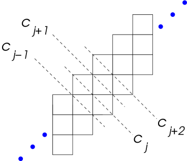
Refer to caption
Figure 5: The coordinate filtration for the 3-strip.

Note that in the figure only the part of the filtration corresponding to the body of the diagram is shown. However, for the head and the tail the principle of cutting the diagram along diagonal lines remains the same, and the filtration is constructed accordingly.

Thus, from the figure it is clear that for the body of the diagram we get two transfer operators repeating periodically in alternation. Denote Ω={(u,v)[0,1]2:u<v}Ωconditional-set𝑢𝑣superscript012𝑢𝑣\Omega=\{(u,v)\in[0,1]^{2}:u<v\}, then the two operators are A:L2[0,1]L2(Ω),B:L2(Ω)L2[0,1]:𝐴subscript𝐿201subscript𝐿2Ω𝐵:subscript𝐿2Ωsubscript𝐿201A:L_{2}[0,1]\to L_{2}(\Omega),B:L_{2}(\Omega)\to L_{2}[0,1] given by

(Af)(u,v)=uvf(x)𝑑x,(Bg)(x)=0xx1g(u,v)𝑑v𝑑u.formulae-sequence𝐴𝑓𝑢𝑣superscriptsubscript𝑢𝑣𝑓𝑥differential-d𝑥𝐵𝑔𝑥superscriptsubscript0𝑥superscriptsubscript𝑥1𝑔𝑢𝑣differential-d𝑣differential-d𝑢(Af)(u,v)=\int_{u}^{v}f(x)dx,\quad(Bg)(x)=\int_{0}^{x}\int_{x}^{1}g(u,v)dv\,du.

Because the composition C:=BAassign𝐶𝐵𝐴C:=B\circ A will repeat periodically, to prove Theorem 1 we will need to diagonalize this operator. We compute:

(Cf)(x)𝐶𝑓𝑥\displaystyle(Cf)(x) =\displaystyle= (B(Af))(x)=0xx1(Af)(u,v)𝑑v𝑑u𝐵𝐴𝑓𝑥superscriptsubscript0𝑥superscriptsubscript𝑥1𝐴𝑓𝑢𝑣differential-d𝑣differential-d𝑢\displaystyle(B(Af))(x)=\int_{0}^{x}\int_{x}^{1}(Af)(u,v)dv\,du
=\displaystyle= 0xx1uvf(y)𝑑y𝑑v𝑑usuperscriptsubscript0𝑥superscriptsubscript𝑥1superscriptsubscript𝑢𝑣𝑓𝑦differential-d𝑦differential-d𝑣differential-d𝑢\displaystyle\int_{0}^{x}\int_{x}^{1}\int_{u}^{v}f(y)dy\,dv\,du
=\displaystyle= 01f(y)(0xy𝑑uxy1𝑑v)𝑑ysuperscriptsubscript01𝑓𝑦superscriptsubscript0𝑥𝑦differential-d𝑢superscriptsubscript𝑥𝑦1differential-d𝑣differential-d𝑦\displaystyle\int_{0}^{1}f(y)\left(\int_{0}^{x\wedge y}du\int_{x\vee y}^{1}dv\right)dy
=\displaystyle= 01f(y)(xy)(1xy)𝑑ysuperscriptsubscript01𝑓𝑦𝑥𝑦1𝑥𝑦differential-d𝑦\displaystyle\int_{0}^{1}f(y)(x\wedge y)(1-x\vee y)dy
=\displaystyle= (1x)0xf(y)y𝑑y+xx1f(y)(1y)𝑑y.1𝑥superscriptsubscript0𝑥𝑓𝑦𝑦differential-d𝑦𝑥superscriptsubscript𝑥1𝑓𝑦1𝑦differential-d𝑦\displaystyle(1-x)\int_{0}^{x}f(y)ydy+x\int_{x}^{1}f(y)(1-y)dy.

Now, to find the eigenfunctions:

λf(x)𝜆𝑓𝑥\displaystyle\lambda f(x) =\displaystyle= (Cf)(x)𝐶𝑓𝑥\displaystyle(Cf)(x) (24)
=\displaystyle= (1x)0xf(y)y𝑑y+xx1f(y)(1y)𝑑y,1𝑥superscriptsubscript0𝑥𝑓𝑦𝑦differential-d𝑦𝑥superscriptsubscript𝑥1𝑓𝑦1𝑦differential-d𝑦\displaystyle(1-x)\int_{0}^{x}f(y)ydy+x\int_{x}^{1}f(y)(1-y)dy,
λf(x)𝜆superscript𝑓𝑥\displaystyle\lambda f^{\prime}(x) =\displaystyle= 01yf(y)𝑑y+x1f(y)𝑑y,superscriptsubscript01𝑦𝑓𝑦differential-d𝑦superscriptsubscript𝑥1𝑓𝑦differential-d𝑦\displaystyle-\int_{0}^{1}yf(y)dy+\int_{x}^{1}f(y)dy,
λf′′(x)𝜆superscript𝑓′′𝑥\displaystyle\lambda f^{\prime\prime}(x) =\displaystyle= f(x).𝑓𝑥\displaystyle-f(x).

From (24) we get the boundary conditions f(0)=f(1)=0𝑓0𝑓10f(0)=f(1)=0. This gives the solutions (scaled to have L2subscript𝐿2L_{2}-norm 111):

ϕk(x)=2sin(πkx),λk=1π2k2,k=1,2,3,formulae-sequencesubscriptitalic-ϕ𝑘𝑥2𝜋𝑘𝑥formulae-sequencesubscript𝜆𝑘1superscript𝜋2superscript𝑘2𝑘123\phi_{k}(x)=\sqrt{2}\sin(\pi kx),\quad\lambda_{k}=\frac{1}{\pi^{2}k^{2}},\quad k=1,2,3,\ldots
Proof of Theorem 1.

We prove (7); the proof of the other formulas is similar and is omitted. If Dnsubscript𝐷𝑛D_{n} is the skew Young diagram appearing in (7), then its associated order polytope is Markovian with respect to the coordinate filtration in Figure 5. One has to be careful at the ends of the diagram; the first and last transfer operators are easily seen to be, respectively,

(Tfirstf)(x)=(Tlastf)(x)=x1f(y)𝑑y.subscript𝑇first𝑓𝑥subscript𝑇last𝑓𝑥superscriptsubscript𝑥1𝑓𝑦differential-d𝑦(T_{\text{first}}f)(x)=(T_{\text{last}}f)(x)=\int_{x}^{1}f(y)dy.

This gives, using Proposition 8 and (23), that the left-hand side of (7) is given by

f(Dn)𝑓subscript𝐷𝑛\displaystyle f(D_{n}) =\displaystyle= (3n)!vol(PDn)=(3n)!Tlast(BA)n1Tfirst𝟏,𝟏3𝑛volsubscript𝑃subscript𝐷𝑛3𝑛subscript𝑇lastsuperscript𝐵𝐴𝑛1subscript𝑇first11\displaystyle(3n)!\mathrm{vol}(P_{D_{n}})=(3n)!\Big{\langle}T_{\text{last}}(BA)^{n-1}T_{\text{first}}{\bf 1},{\bf 1}\Big{\rangle}
=\displaystyle= (3n)!Cn1(1x),x3𝑛superscript𝐶𝑛11𝑥𝑥\displaystyle(3n)!\Big{\langle}C^{n-1}(1-x),x\Big{\rangle}
=\displaystyle= (3n)!k=1λkn1x,ϕk1x,ϕk3𝑛superscriptsubscript𝑘1superscriptsubscript𝜆𝑘𝑛1𝑥subscriptitalic-ϕ𝑘1𝑥subscriptitalic-ϕ𝑘\displaystyle(3n)!\sum_{k=1}^{\infty}\lambda_{k}^{n-1}\Big{\langle}x,\phi_{k}\Big{\rangle}\Big{\langle}1-x,\phi_{k}\Big{\rangle}

A quick computation gives that x,ϕk=2(1)k1/πk𝑥subscriptitalic-ϕ𝑘2superscript1𝑘1𝜋𝑘\Big{\langle}x,\phi_{k}\Big{\rangle}=\sqrt{2}(-1)^{k-1}/\pi k, 1x,ϕk=2/πk1𝑥subscriptitalic-ϕ𝑘2𝜋𝑘\Big{\langle}1-x,\phi_{k}\Big{\rangle}=\sqrt{2}/\pi k, so

f(Dn)=(3n)!k=1(1)k12π2k2(πk)2(n1)=2(3n)!π2n(1222n)ζ(2n)𝑓subscript𝐷𝑛3𝑛superscriptsubscript𝑘1superscript1𝑘12superscript𝜋2superscript𝑘2superscript𝜋𝑘2𝑛123𝑛superscript𝜋2𝑛12superscript22𝑛𝜁2𝑛f(D_{n})=(3n)!\sum_{k=1}^{\infty}\frac{(-1)^{k-1}2}{\pi^{2}k^{2}(\pi k)^{2(n-1)}}=\frac{2(3n)!}{\pi^{2n}}\left(1-\frac{2}{2^{2n}}\right)\zeta(2n)

(where as usual ζ(x)=n=1nx𝜁𝑥superscriptsubscript𝑛1superscript𝑛𝑥\zeta(x)=\sum_{n=1}^{\infty}n^{-x}). Now substituting the classical identity

ζ(2n)=k=11k2n=(1)n1π2n22n1B2n(2n)!𝜁2𝑛superscriptsubscript𝑘11superscript𝑘2𝑛superscript1𝑛1superscript𝜋2𝑛superscript22𝑛1subscript𝐵2𝑛2𝑛\zeta(2n)=\sum_{k=1}^{\infty}\frac{1}{k^{2n}}=\frac{(-1)^{n-1}\pi^{2n}2^{2n-1}B_{2n}}{(2n)!} (25)

(together with (3)) gives (7). ∎

5 The 4-strip

While the analysis so far has been relatively straightforward, the case of the 444-strip is the first case where one encounters relative difficulty in diagonalizing the transfer operator, which now works on a 2-dimensional domain. As before, we choose the coordinate filtration obtained by cutting the diagram along diagonal lines, as shown in the figure below.
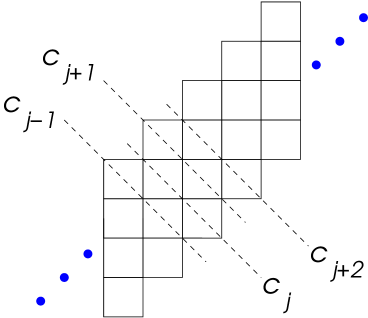
Refer to caption
Figure 6: The coordinate filtration for the 4-strip.

Again, we get the following two transfer operators repeating periodically in alternation. Denote as before Ω={(u,v)[0,1]2:u<v}Ωconditional-set𝑢𝑣superscript012𝑢𝑣\Omega=\{(u,v)\in[0,1]^{2}:u<v\}, then we have that A,B:L2(Ω)L2(Ω):𝐴𝐵subscript𝐿2Ωsubscript𝐿2ΩA,B:L_{2}(\Omega)\to L_{2}(\Omega) are given by

(Af)(x,y)𝐴𝑓𝑥𝑦\displaystyle(Af)(x,y) =\displaystyle= 0xxyf(u,v)𝑑v𝑑u,superscriptsubscript0𝑥superscriptsubscript𝑥𝑦𝑓𝑢𝑣differential-d𝑣differential-d𝑢\displaystyle\int_{0}^{x}\int_{x}^{y}f(u,v)dv\,du,
(Bg)(u,v)𝐵𝑔𝑢𝑣\displaystyle(Bg)(u,v) =\displaystyle= uvv1g(x,y)𝑑x𝑑y.superscriptsubscript𝑢𝑣superscriptsubscript𝑣1𝑔𝑥𝑦differential-d𝑥differential-d𝑦\displaystyle\int_{u}^{v}\int_{v}^{1}g(x,y)dx\,dy.

A small simplification is to note that there is a certain symmetry, in that A𝐴A and B𝐵B are conjugate to each other: B=CAC𝐵𝐶𝐴𝐶B=CAC, where C:L2(Ω)L2(Ω):𝐶subscript𝐿2Ωsubscript𝐿2ΩC:L_{2}(\Omega)\to L_{2}(\Omega) is the reflection operator

(Cf)(x,y)=f(1y,1x).𝐶𝑓𝑥𝑦𝑓1𝑦1𝑥(Cf)(x,y)=f(1-y,1-x).

So, instead of diagonalizing the composition BA=CACA𝐵𝐴𝐶𝐴𝐶𝐴BA=CACA we can diagonalize its simpler “square root” CA𝐶𝐴CA, given by

(CAf)(x,y)=01y1y1xf(u,v)𝑑v𝑑u.𝐶𝐴𝑓𝑥𝑦superscriptsubscript01𝑦superscriptsubscript1𝑦1𝑥𝑓𝑢𝑣differential-d𝑣differential-d𝑢(CAf)(x,y)=\int_{0}^{1-y}\int_{1-y}^{1-x}f(u,v)dv\,du. (26)

So we are looking for λ,f𝜆𝑓\lambda,f which are solutions of

λf(x,y)=01y1y1xf(u,v)𝑑v𝑑u.𝜆𝑓𝑥𝑦superscriptsubscript01𝑦superscriptsubscript1𝑦1𝑥𝑓𝑢𝑣differential-d𝑣differential-d𝑢\lambda f(x,y)=\int_{0}^{1-y}\int_{1-y}^{1-x}f(u,v)dv\,du.

Differentiating once with respect to each variable gives

λ2fxy=f(1y,1x).𝜆superscript2𝑓𝑥𝑦𝑓1𝑦1𝑥\lambda\frac{\partial^{2}f}{\partial x\partial y}=f(1-y,1-x). (27)

Differentiating again w.r.t. x,y𝑥𝑦x,y and substituting in (27) gives the PDE

4f2x2y=1λ2f(x,y).superscript4𝑓superscript2𝑥superscript2𝑦1superscript𝜆2𝑓𝑥𝑦\frac{\partial^{4}f}{\partial^{2}x\partial^{2}y}=\frac{1}{\lambda^{2}}f(x,y). (28)

The boundary conditions are easily seen to be

f(x,1)0,f(x,x)0,fx(0,y)0,formulae-sequence𝑓𝑥10formulae-sequence𝑓𝑥𝑥0subscript𝑓𝑥0𝑦0f(x,1)\equiv 0,\quad f(x,x)\equiv 0,\quad f_{x}(0,y)\equiv 0, (29)

a mixture of Dirichlet- and Neumann-type conditions on the three boundary sides of ΩΩ\Omega.

Now, it may be verified that the L2subscript𝐿2L_{2}-normalized solutions to this boundary value problem are given by

ϕj,k(x,y)subscriptitalic-ϕ𝑗𝑘𝑥𝑦\displaystyle\phi_{j,k}(x,y) =\displaystyle= 2det(cos(π(2j1)x2)cos(π(2j1)y2)cos(π(2k1)x2)cos(π(2k1)y2)),2𝜋2𝑗1𝑥2𝜋2𝑗1𝑦2𝜋2𝑘1𝑥2𝜋2𝑘1𝑦2\displaystyle 2\det\left(\begin{array}[]{ll}\cos\left(\frac{\pi(2j-1)x}{2}\right)&\cos\left(\frac{\pi(2j-1)y}{2}\right)\\ \cos\left(\frac{\pi(2k-1)x}{2}\right)&\cos\left(\frac{\pi(2k-1)y}{2}\right)\end{array}\right), (31)
λj,ksubscript𝜆𝑗𝑘\displaystyle\lambda_{j,k} =\displaystyle= 4(1)j+k1π2(2j1)(2k1),k>j>0 integers,4superscript1𝑗𝑘1superscript𝜋22𝑗12𝑘1𝑘𝑗0 integers\displaystyle\frac{4(-1)^{j+k-1}}{\pi^{2}(2j-1)(2k-1)},\qquad k>j>0\text{ integers}, (32)

(note that the eigenfunctions are parametrized by two integers). While verification is easy, two related questions that should be addressed are: how these solutions can be derived rather than guessed; and how to prove that these solutions span all eigenspaces. We answer the first question and then point out how this essentially contains the answer to the second. The PDE (28) is of a very simple form that suggests trying to use Fourier series and the method of separation of variables. However, the domain ΩΩ\Omega is not of a shape suitable for the application of this method. But looking at the boundary conditions (29) suggests looking for a function on a larger domain that satisfies the symmetry and anti-symmetry conditions

f(y,x)𝑓𝑦𝑥\displaystyle f(y,x) =\displaystyle= f(x,y),𝑓𝑥𝑦\displaystyle-f(x,y),
f(x,y)𝑓𝑥𝑦\displaystyle f(-x,y) =\displaystyle= f(x,y)=f(x,y),𝑓𝑥𝑦𝑓𝑥𝑦\displaystyle f(x,-y)=f(x,y), (33)
f(x,2y)𝑓𝑥2𝑦\displaystyle f(x,2-y) =\displaystyle= f(2x,y)=f(x,y)𝑓2𝑥𝑦𝑓𝑥𝑦\displaystyle f(2-x,y)=-f(x,y)

since such a function will automatically satisfy (29). Now, any function satisfying (33) is periodic in both variables with period 4, i.e., satisfies f(x+4,y)=f(x,y+4)=f(x,y)𝑓𝑥4𝑦𝑓𝑥𝑦4𝑓𝑥𝑦f(x+4,y)=f(x,y+4)=f(x,y), and its values everywhere are determined by its values on ΩΩ\Omega. Thus one gets a problem suitable for the application of the method of separation of variables: Expand f𝑓f in a Fourier series

f(x,y)=a,bca,bexp(πi2(ax+by)).𝑓𝑥𝑦subscript𝑎𝑏subscript𝑐𝑎𝑏𝜋𝑖2𝑎𝑥𝑏𝑦f(x,y)=\sum_{a,b\in\mathbb{Z}}c_{a,b}\exp\left(\frac{\pi i}{2}(ax+by)\right).

The symmetry conditions (33) translate to the following equations on the coefficients ca,bsubscript𝑐𝑎𝑏c_{a,b}:

ca,b=ca,b,ca,b=ca,b,cb,a=ca,b,formulae-sequencesubscript𝑐𝑎𝑏subscript𝑐𝑎𝑏formulae-sequencesubscript𝑐𝑎𝑏subscript𝑐𝑎𝑏subscript𝑐𝑏𝑎subscript𝑐𝑎𝑏c_{-a,b}=c_{a,b},\quad c_{a,-b}=c_{a,b},\quad c_{b,a}=-c_{a,b},
ca,b=(1)b+1ca,b,ca,b=(1)a+1ca,b.formulae-sequencesubscript𝑐𝑎𝑏superscript1𝑏1subscript𝑐𝑎𝑏subscript𝑐𝑎𝑏superscript1𝑎1subscript𝑐𝑎𝑏c_{a,b}=(-1)^{b+1}c_{a,b},\quad c_{a,b}=(-1)^{a+1}c_{a,b}.

In particular the last conditions imply that a,b𝑎𝑏a,b are odd if ca,b0subscript𝑐𝑎𝑏0c_{a,b}\neq 0. Eq. (27) implies the additional equation

π24λabca,b=ia+bca,b,superscript𝜋24𝜆𝑎𝑏subscript𝑐𝑎𝑏superscript𝑖𝑎𝑏subscript𝑐𝑎𝑏-\frac{\pi^{2}}{4}\lambda ab\,c_{a,b}=-i^{a+b}c_{a,b},

Denoting λ=4ia+b/π2ab𝜆4superscript𝑖𝑎𝑏superscript𝜋2𝑎𝑏\lambda=4i^{a+b}/\pi^{2}ab for some (and therefore all) a,b𝑎𝑏a,b for which ca,b0subscript𝑐𝑎𝑏0c_{a,b}\neq 0, it is easy to verify from these relations that f𝑓f is a linear combination of the functions ϕj,ksubscriptitalic-ϕ𝑗𝑘\phi_{j,k} with k>j>0𝑘𝑗0k>j>0 and |ab|=(2j1)(2k1)𝑎𝑏2𝑗12𝑘1|ab|=(2j-1)(2k-1) (note that some eigenvalues do have multiplicity greater than 1, corresponding to different representations of |ab|𝑎𝑏|ab| as products of distinct odd positive integers).

It remains to answer the second question posed above, of showing that the system (32) is indeed a complete eigensystem for the operator CA𝐶𝐴CA . The answer is encoded in the previous discussion, but one has to argue more formally now. Let X𝑋X be the subset of L2([2,2]2)subscript𝐿2superscript222L_{2}([-2,2]^{2}) of functions satisfying the symmetry conditions (33), and let Y𝑌Y be the subset of L2(Ω)subscript𝐿2ΩL_{2}(\Omega) of functions satisfying the boundary conditions (29). Let D𝐷D be the linear operator on X𝑋X given by

(Df)(x,y)=01y01xf(u,v)𝑑v𝑑u,𝐷𝑓𝑥𝑦superscriptsubscript01𝑦superscriptsubscript01𝑥𝑓𝑢𝑣differential-d𝑣differential-d𝑢(Df)(x,y)=\int_{0}^{1-y}\int_{0}^{1-x}f(u,v)dv\,du, (34)

manifestly a compact self-adjoint operator.

Note that Df𝐷𝑓Df can be also defined by the right-hand side of (26) due to the symmetry conditions imposed on elements of X𝑋X. Let P:XY:𝑃𝑋𝑌P:X\to Y be defined by Pf=f|ΩPf=f_{|\Omega}. Then P𝑃P is clearly an isomorphism of Hilbert spaces, and D𝐷D is conjugate to CA𝐶𝐴CA under P𝑃P, i.e., CA=PDP1𝐶𝐴𝑃𝐷superscript𝑃1CA=PDP^{-1}. Therefore fY𝑓𝑌f\in Y is an eigenfunction of CA𝐶𝐴CA iff P1fsuperscript𝑃1𝑓P^{-1}f is an eigenfunction of D𝐷D. As the eigenfunctions of D𝐷D form a complete orthonormal system in X𝑋X, we have proved:

Proposition 9.

The system (32) is a complete normalized eigensystem for the operator CA𝐶𝐴CA.

Proof of Theorem 2.

Denote by Fnsubscript𝐹𝑛F_{n} and Gnsubscript𝐺𝑛G_{n} the skew Young diagrams appearing on the left-hand sides of (8), (9), respectively. Following the same reasoning as before using Proposition 8 and (23), we have that

f(Fn)𝑓subscript𝐹𝑛\displaystyle f(F_{n}) =\displaystyle= (4n2)!(CA)2n3(yx),yx,4𝑛2superscript𝐶𝐴2𝑛3𝑦𝑥𝑦𝑥\displaystyle(4n-2)!\Big{\langle}(CA)^{2n-3}(y-x),y-x\Big{\rangle},
f(Gn)𝑓subscript𝐺𝑛\displaystyle f(G_{n}) =\displaystyle= (4n)!(CA)2n3(y2x22),y2x22.4𝑛superscript𝐶𝐴2𝑛3superscript𝑦2superscript𝑥22superscript𝑦2superscript𝑥22\displaystyle(4n)!\Big{\langle}(CA)^{2n-3}\left(\frac{y^{2}-x^{2}}{2}\right),\frac{y^{2}-x^{2}}{2}\Big{\rangle}.

Using these formulas and Proposition 9, after a computation one finally arrives at (8), (9), using (25) and another classical identity due to Euler, namely

k=1(1)k1(2k1)2n+1=(1)nπ2n+1E2n22n+2(2n)!.superscriptsubscript𝑘1superscript1𝑘1superscript2𝑘12𝑛1superscript1𝑛superscript𝜋2𝑛1subscript𝐸2𝑛superscript22𝑛22𝑛\sum_{k=1}^{\infty}\frac{(-1)^{k-1}}{(2k-1)^{2n+1}}=\frac{(-1)^{n}\pi^{2n+1}E_{2n}}{2^{2n+2}(2n)!}.

We leave verification of these straightforward details to the reader. Also note that these computations are superseded by our more general proof of Theorem 4 in Section 8. ∎

6 The 2k2𝑘2k-strip and the (2k+1)2𝑘1(2k+1)-strip

Having analyzed the case of 444-strip diagrams, the results are now easily generalized to the 2k2𝑘2k-strip and the (2k+1)2𝑘1(2k+1). Here are the results for the 2k2𝑘2k-strip. The coordinate filtration is again constructed by cutting the diagram along diagonals. This leads to a transfer operator on L2(Ωk)subscript𝐿2subscriptΩ𝑘L_{2}(\Omega_{k}), where

Ωk={x[0,1]k:x1x2xk}.subscriptΩ𝑘conditional-set𝑥superscript01𝑘subscript𝑥1subscript𝑥2subscript𝑥𝑘\Omega_{k}=\Big{\{}x\in[0,1]^{k}:x_{1}\leq x_{2}\leq\ldots\leq x_{k}\Big{\}}.

The transfer operator is given by

(S2kf)(x1,,xk)=01xk1xk1xk11xk11xk21x21x1f(y1,,yk)𝑑yk𝑑yk1𝑑y1.subscript𝑆2𝑘𝑓subscript𝑥1subscript𝑥𝑘superscriptsubscript01subscript𝑥𝑘superscriptsubscript1subscript𝑥𝑘1subscript𝑥𝑘1superscriptsubscript1subscript𝑥𝑘11subscript𝑥𝑘2superscriptsubscript1subscript𝑥21subscript𝑥1𝑓subscript𝑦1subscript𝑦𝑘differential-dsubscript𝑦𝑘differential-dsubscript𝑦𝑘1differential-dsubscript𝑦1(S_{2k}f)(x_{1},\ldots,x_{k})=\\ \int_{0}^{1-x_{k}}\int_{1-x_{k}}^{1-x_{k-1}}\int_{1-x_{k-1}}^{1-x_{k-2}}\ldots\int_{1-x_{2}}^{1-x_{1}}f(y_{1},\ldots,y_{k})dy_{k}\,dy_{k-1}\,\ldots\,dy_{1}. (35)

In this representation we have already taken advantage of the symmetry using the “square root” trick as in the case of the 4-strip to reduce two conjugate transfer operators repeating in alternation to a single operator. Diagonalizing S2ksubscript𝑆2𝑘S_{2k} leads to the following boundary value problem:

kf(x1,x2,,xk)x1x2xk=(1)kλf(1xk,,1x2,1x1),superscript𝑘𝑓subscript𝑥1subscript𝑥2subscript𝑥𝑘subscript𝑥1subscript𝑥2subscript𝑥𝑘superscript1𝑘𝜆𝑓1subscript𝑥𝑘1subscript𝑥21subscript𝑥1\frac{\partial^{k}f(x_{1},x_{2},\ldots,x_{k})}{\partial x_{1}\partial x_{2}\ldots\partial x_{k}}=\frac{(-1)^{k}}{\lambda}f(1-x_{k},\ldots,1-x_{2},1-x_{1}),
f𝑓\displaystyle f \displaystyle\equiv 0 on x1x2,x2x3,,xk1xk,xk1,formulae-sequence0 on subscript𝑥1subscript𝑥2formulae-sequencesubscript𝑥2subscript𝑥3formulae-sequencesubscript𝑥𝑘1subscript𝑥𝑘subscript𝑥𝑘1\displaystyle 0\text{ on }x_{1}\equiv x_{2},x_{2}\equiv x_{3},\ldots,x_{k-1}\equiv x_{k},x_{k}\equiv 1,
fx1subscript𝑓subscript𝑥1\displaystyle f_{x_{1}} \displaystyle\equiv 0 on x10.0 on subscript𝑥10\displaystyle 0\text{ on }x_{1}\equiv 0.

The ideas of Section 5 can be used to prove:

Theorem 10 (Diagonalization of the 2k2𝑘2k-strip transfer operator).

The system of functions and associated eigenvalues

ϕj1,,jk(x1,,xk)subscriptitalic-ϕsubscript𝑗1subscript𝑗𝑘subscript𝑥1subscript𝑥𝑘\displaystyle\phi_{j_{1},\ldots,j_{k}}(x_{1},\ldots,x_{k}) =\displaystyle= 2k/2det(cos(π(2jp1)xq2))1p,qk,superscript2𝑘2subscript𝜋2subscript𝑗𝑝1subscript𝑥𝑞2formulae-sequence1𝑝𝑞𝑘\displaystyle 2^{k/2}\det\left(\cos\left(\frac{\pi(2j_{p}-1)x_{q}}{2}\right)\right)_{1\leq p,q\leq k},
λj1,,jksubscript𝜆subscript𝑗1subscript𝑗𝑘\displaystyle\lambda_{j_{1},\ldots,j_{k}} =\displaystyle= 2k(1)(k2)+p(jp+1)πk(2j11)(2j21)(2jk1),superscript2𝑘superscript1binomial𝑘2subscript𝑝subscript𝑗𝑝1superscript𝜋𝑘2subscript𝑗112subscript𝑗212subscript𝑗𝑘1\displaystyle\frac{2^{k}(-1)^{\binom{k}{2}+\sum_{p}(j_{p}+1)}}{\pi^{k}(2j_{1}-1)(2j_{2}-1)\ldots(2j_{k}-1)},
j1>j2>>jk>0 integers,subscript𝑗1subscript𝑗2subscript𝑗𝑘0 integers,\displaystyle\ j_{1}>j_{2}>\ldots>j_{k}>0\text{ integers,}

is a complete orthonormal eigensystem for the operator S2ksubscript𝑆2𝑘S_{2k} in (35).

For the (2k+1)2𝑘1(2k+1)-strip, we have similar results generalizing the analysis of Section 4. In this case, we have two operators A:L2(Ωk+1)L2(Ωk),B:L2(Ωk)L2(Ωk+1):𝐴subscript𝐿2subscriptΩ𝑘1subscript𝐿2subscriptΩ𝑘𝐵:subscript𝐿2subscriptΩ𝑘subscript𝐿2subscriptΩ𝑘1A:L_{2}(\Omega_{k+1})\to L_{2}(\Omega_{k}),B:L_{2}(\Omega_{k})\to L_{2}(\Omega_{k+1}) given by

(Ag)(x1,,xk)=0x1x1x2x2x3xk1xkxk1g(y1,,yk+1)𝑑yk+1𝑑y1,𝐴𝑔subscript𝑥1subscript𝑥𝑘superscriptsubscript0subscript𝑥1superscriptsubscriptsubscript𝑥1subscript𝑥2superscriptsubscriptsubscript𝑥2subscript𝑥3superscriptsubscriptsubscript𝑥𝑘1subscript𝑥𝑘superscriptsubscriptsubscript𝑥𝑘1𝑔subscript𝑦1subscript𝑦𝑘1differential-dsubscript𝑦𝑘1differential-dsubscript𝑦1(Ag)(x_{1},\ldots,x_{k})=\\ \int_{0}^{x_{1}}\int_{x_{1}}^{x_{2}}\int_{x_{2}}^{x_{3}}\ldots\int_{x_{k-1}}^{x_{k}}\int_{x_{k}}^{1}g(y_{1},\ldots,y_{k+1})dy_{k+1}\,\ldots\,dy_{1},
(Bh)(y1,,yk+1)=y1y2y2y3y3y4ykyk+1h(x1,,xk)𝑑xk𝑑x1.𝐵subscript𝑦1subscript𝑦𝑘1superscriptsubscriptsubscript𝑦1subscript𝑦2superscriptsubscriptsubscript𝑦2subscript𝑦3superscriptsubscriptsubscript𝑦3subscript𝑦4superscriptsubscriptsubscript𝑦𝑘subscript𝑦𝑘1subscript𝑥1subscript𝑥𝑘differential-dsubscript𝑥𝑘differential-dsubscript𝑥1\ \ (Bh)(y_{1},\ldots,y_{k+1})\ =\\ \int_{y_{1}}^{y_{2}}\int_{y_{2}}^{y_{3}}\int_{y_{3}}^{y_{4}}\ldots\int_{y_{k}}^{y_{k+1}}h(x_{1},\ldots,x_{k})dx_{k}\,\ldots\,dx_{1}.

The relevant operator to diagonalize is the composition AB𝐴𝐵AB. This leads to the following boundary value problem:

2kf2x12x22xk=1λ2f,f|Ωk0\frac{\partial^{2k}f}{\partial^{2}x_{1}\partial^{2}x_{2}\ldots\partial^{2}x_{k}}=\frac{1}{\lambda^{2}}f,\qquad f_{\big{|}\partial\Omega_{k}}\equiv 0

The solution is given by the following theorem.

Theorem 11 (Diagonalization of the (2k+1)2𝑘1(2k+1)-strip transfer operator).

The system of functions and associated eigenvalues

ϕj1,,jk(x1,,xk)subscriptitalic-ϕsubscript𝑗1subscript𝑗𝑘subscript𝑥1subscript𝑥𝑘\displaystyle\phi_{j_{1},\ldots,j_{k}}(x_{1},\ldots,x_{k}) =\displaystyle= 2k/2det(sin(πjpxq))1p,qk,superscript2𝑘2subscript𝜋subscript𝑗𝑝subscript𝑥𝑞formulae-sequence1𝑝𝑞𝑘\displaystyle 2^{k/2}\det\Big{(}\sin\left(\pi j_{p}x_{q}\right)\Big{)}_{1\leq p,q\leq k},
λj1,,jksubscript𝜆subscript𝑗1subscript𝑗𝑘\displaystyle\lambda_{j_{1},\ldots,j_{k}} =\displaystyle= 1π2kj12j22jk2,1superscript𝜋2𝑘superscriptsubscript𝑗12superscriptsubscript𝑗22superscriptsubscript𝑗𝑘2\displaystyle\frac{1}{\pi^{2k}j_{1}^{2}j_{2}^{2}\ldots j_{k}^{2}},
j1>j2>>jk>0 integers,subscript𝑗1subscript𝑗2subscript𝑗𝑘0 integers,\displaystyle j_{1}>j_{2}>\ldots>j_{k}>0\text{ integers,}

is a complete orthonormal eigensystem for the operator AB𝐴𝐵AB.

7 A Schur function identity

In this section, we prove an identity that will be used in the next section in the proof of Theorem 4.

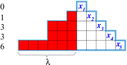
Let λ=(λ1λ2λk0)𝜆subscript𝜆1subscript𝜆2subscript𝜆𝑘0\lambda=\left(\lambda_{1}\geq\lambda_{2}\geq\ldots\geq\lambda_{k}\geq 0\right) be a Young diagram, possibly with some parts being 0. Consider the head (or tail) polytope Pλsubscript𝑃𝜆P_{\lambda}, defined by the system of linear inequalities:

0yi,j10subscript𝑦𝑖𝑗1\displaystyle 0\leq y_{i,j}\leq 1 1ik,(ki)jλi,formulae-sequence1𝑖𝑘𝑘𝑖𝑗subscript𝜆𝑖\displaystyle 1\leq i\leq k,\ \ -(k-i)\leq j\leq\lambda_{i},
yi,jyi+1,jsubscript𝑦𝑖𝑗subscript𝑦𝑖1𝑗\displaystyle y_{i,j}\geq y_{i+1,j} where defined,
yi,jyi,j+1subscript𝑦𝑖𝑗subscript𝑦𝑖𝑗1\displaystyle y_{i,j}\geq y_{i,j+1} where defined,

and for 𝐱=(x1,,xk)𝐱subscript𝑥1subscript𝑥𝑘{\bf x}=(x_{1},\ldots,x_{k}) in the simplex ΩksubscriptΩ𝑘\Omega_{k}, denote by Pλ(𝐱)subscript𝑃𝜆𝐱P_{\lambda}({\bf x}) the section

Pλ(𝐱)={yPλ:yk+1i,(i1)=xi,i=1,2,,k}subscript𝑃𝜆𝐱conditional-set𝑦subscript𝑃𝜆formulae-sequencesubscript𝑦𝑘1𝑖𝑖1subscript𝑥𝑖𝑖12𝑘P_{\lambda}({\bf x})=\Big{\{}y\in P_{\lambda}:y_{k+1-i,-(i-1)}=x_{i},\ \ i=1,2,\ldots,k\Big{\}}

(see Figure 7).

Refer to caption
Figure 7: The polytope Pλsubscript𝑃𝜆P_{\lambda} is the order polytope of the diagram (which is not a skew Young diagram) formed by leaning the Young diagram λ𝜆\lambda against a triangular (“staircase”) diagram, and Pλ(𝐱)subscript𝑃𝜆𝐱P_{\lambda}({\bf x}) is its section where the values along the main diagonal are x1,,xksubscript𝑥1subscript𝑥𝑘x_{1},\ldots,x_{k}. In this example λ=(6,3,3,1,0)𝜆63310\lambda=(6,3,3,1,0).

Obviously, the volume of Pλ(𝐱)subscript𝑃𝜆𝐱P_{\lambda}({\bf x}) is a polynomial function on the simplex ΩksubscriptΩ𝑘\Omega_{k}. More precisely:

Proposition 12.

Let Li=λi+ki, 1ikformulae-sequencesubscript𝐿𝑖subscript𝜆𝑖𝑘𝑖1𝑖𝑘L_{i}=\lambda_{i}+k-i,\ \ 1\leq i\leq k. The volume of the polytope Pλ(𝐱)subscript𝑃𝜆𝐱P_{\lambda}({\bf x}) (of the appropriate dimensionality) is

vol(Pλ(𝐱))=1i=1kLi!det(xiLj)1i,jksubscriptvolsubscript𝑃𝜆𝐱1superscriptsubscriptproduct𝑖1𝑘subscript𝐿𝑖subscriptsuperscriptsubscript𝑥𝑖subscript𝐿𝑗formulae-sequence1𝑖𝑗𝑘\mathrm{vol}_{*}(P_{\lambda}({\bf x}))=\frac{1}{\prod_{i=1}^{k}L_{i}!}\det\left(x_{i}^{L_{j}}\right)_{1\leq i,j\leq k} (36)

Proposition 12 generalizes a well-known fact corresponding to the case λ=(0,0,,0)𝜆000\lambda=(0,0,\ldots,0), see for example [6, Lemma 1.12] and [11, Section 4]. It is known to experts, though perhaps in a slightly different form, and can be proved using the Karlin-McGregor theory of non-intersecting paths. We will give a direct proof by induction. Note that the expression on the right-hand side of (36) is equal to (i=1kLi!)1sλ(𝐱)V(𝐱)superscriptsuperscriptsubscriptproduct𝑖1𝑘subscript𝐿𝑖1subscript𝑠𝜆𝐱𝑉𝐱\left(\prod_{i=1}^{k}L_{i}!\right)^{-1}s_{\lambda}({\bf x})V({\bf x}), where sλsubscript𝑠𝜆s_{\lambda} is the Schur symmetric function associated to λ𝜆\lambda and V(𝐱)=i<j(xixj)𝑉𝐱subscriptproduct𝑖𝑗subscript𝑥𝑖subscript𝑥𝑗V({\bf x})=\prod_{i<j}(x_{i}-x_{j}) is the Vandermonde determinant.

Proof.

We will proceed by induction on |λ|+k𝜆𝑘|\lambda|+k (where |λ|=λ1++λk𝜆subscript𝜆1subscript𝜆𝑘|\lambda|=\lambda_{1}+\ldots+\lambda_{k}). The induction base is trivial. For the inductive step, we divide into two cases according to whether λk>0subscript𝜆𝑘0\lambda_{k}>0 or λk=0subscript𝜆𝑘0\lambda_{k}=0. In the former case, the inductive hypothesis holds for the smaller Young diagram

λ=(λ11,λ21,,λk1),superscript𝜆subscript𝜆11subscript𝜆21subscript𝜆𝑘1\lambda^{\prime}=\left(\lambda_{1}-1,\lambda_{2}-1,\ldots,\lambda_{k}-1\right),

and the volume of the polytope Pλ(𝐱)subscript𝑃𝜆𝐱P_{\lambda}({\bf x}) can be represented as

0x1x1x2xk1xkvol[Pλ(y1,,yk)]𝑑yk𝑑yk1𝑑y1superscriptsubscript0subscript𝑥1superscriptsubscriptsubscript𝑥1subscript𝑥2superscriptsubscriptsubscript𝑥𝑘1subscript𝑥𝑘subscriptvoldelimited-[]subscript𝑃superscript𝜆subscript𝑦1subscript𝑦𝑘differential-dsubscript𝑦𝑘differential-dsubscript𝑦𝑘1differential-dsubscript𝑦1\int_{0}^{x_{1}}\int_{x_{1}}^{x_{2}}\ldots\int_{x_{k-1}}^{x_{k}}\mathrm{vol}_{*}[P_{\lambda^{\prime}}(y_{1},\ldots,y_{k})]dy_{k}\,dy_{k-1}\ldots dy_{1} (37)

(this is essentiallly a transfer operator computation, since the diagram formed by λ𝜆\lambda with its adjoining triangular part can be obtained from the corresponding diagram for λsuperscript𝜆\lambda^{\prime} by adding one diagonal). Using the inductive hypothesis, the integrand is antisymmetric, and therefore the expression in (37) can be rewritten as

0x10x20xkvol[Pλ(y1,,yk)]𝑑yk𝑑yk1𝑑y1superscriptsubscript0subscript𝑥1superscriptsubscript0subscript𝑥2superscriptsubscript0subscript𝑥𝑘subscriptvoldelimited-[]subscript𝑃superscript𝜆subscript𝑦1subscript𝑦𝑘differential-dsubscript𝑦𝑘differential-dsubscript𝑦𝑘1differential-dsubscript𝑦1\int_{0}^{x_{1}}\int_{0}^{x_{2}}\ldots\int_{0}^{x_{k}}\mathrm{vol}_{*}[P_{\lambda^{\prime}}(y_{1},\ldots,y_{k})]dy_{k}\,dy_{k-1}\ldots dy_{1} (38)

(similar reasoning was used in the proof of Proposition 9), which in turn, again by the inductive hypothesis, is equal to

0x10xkdet(1(Lj1)!yiLj1)i,jdykdy1superscriptsubscript0subscript𝑥1superscriptsubscript0subscript𝑥𝑘subscript1subscript𝐿𝑗1superscriptsubscript𝑦𝑖subscript𝐿𝑗1𝑖𝑗𝑑subscript𝑦𝑘𝑑subscript𝑦1\displaystyle\int_{0}^{x_{1}}\ldots\int_{0}^{x_{k}}\det\left(\frac{1}{(L_{j}-1)!}y_{i}^{L_{j}-1}\right)_{i,j}dy_{k}\ldots dy_{1}\qquad\qquad
=det(1Lj!xiLj)i,j,subscript1subscript𝐿𝑗superscriptsubscript𝑥𝑖subscript𝐿𝑗𝑖𝑗\displaystyle=\ \ \det\left(\frac{1}{L_{j}!}x_{i}^{L_{j}}\right)_{i,j},\qquad\qquad\qquad\qquad\qquad\qquad\qquad (39)

proving the inductive step in this case.

The other induction step deals with the second case where λk=0subscript𝜆𝑘0\lambda_{k}=0. Here, we use the inductive hypothesis for the Young diagram

λ=(λ1,,λk1)superscript𝜆subscript𝜆1subscript𝜆𝑘1\lambda^{\prime}=(\lambda_{1},\ldots,\lambda_{k-1})

(the same diagram, but we attach to it a smaller triangle of order k1𝑘1k-1 only). The relation between the two polytopes Pλ(𝐱),Pλ(𝐲)subscript𝑃𝜆𝐱subscript𝑃superscript𝜆𝐲P_{\lambda}({\bf x}),P_{\lambda^{\prime}}({\bf y}) can be seen (again using an iterated integral which is really a transfer operator computation) to be

vol(Pλ(𝐱))=x1x2x1x3x1xkvol(Pλ(y2,,yk))𝑑yk𝑑y3𝑑y2.subscriptvolsubscript𝑃𝜆𝐱superscriptsubscriptsubscript𝑥1subscript𝑥2superscriptsubscriptsubscript𝑥1subscript𝑥3superscriptsubscriptsubscript𝑥1subscript𝑥𝑘subscriptvolsubscript𝑃superscript𝜆subscript𝑦2subscript𝑦𝑘differential-dsubscript𝑦𝑘differential-dsubscript𝑦3differential-dsubscript𝑦2\mathrm{vol}_{*}(P_{\lambda}({\bf x}))=\!\int_{x_{1}}^{x_{2}}\!\int_{x_{1}}^{x_{3}}\!\ldots\!\int_{x_{1}}^{x_{k}}\!\!\mathrm{vol}_{*}(P_{\lambda^{\prime}}(y_{2},\ldots,y_{k}))dy_{k}\ldots dy_{3}\,dy_{2}.

This can be dealt with similarly to (39), simplifying eventually to the expression

1i=1k1Li!det(x1L1x2L1xkL1x1Lk1x2Lk1xkLk1111)1superscriptsubscriptproduct𝑖1𝑘1subscript𝐿𝑖superscriptsubscript𝑥1subscript𝐿1superscriptsubscript𝑥2subscript𝐿1superscriptsubscript𝑥𝑘subscript𝐿1missing-subexpressionsuperscriptsubscript𝑥1subscript𝐿𝑘1superscriptsubscript𝑥2subscript𝐿𝑘1superscriptsubscript𝑥𝑘subscript𝐿𝑘1111\frac{1}{\prod_{i=1}^{k-1}L_{i}!}\det\left(\begin{array}[]{llll}x_{1}^{L_{1}}&x_{2}^{L_{1}}&\ldots&x_{k}^{L_{1}}\\ \vdots&\vdots&&\vdots\\ x_{1}^{L_{k-1}}&x_{2}^{L_{k-1}}&\ldots&x_{k}^{L_{k-1}}\\ 1&1&\ldots&1\end{array}\right)

which is exactly the right-hand side of (36) (since Lk=0subscript𝐿𝑘0L_{k}=0 in this induction step). ∎

It is worth noting that this proof, similarly to the computations in the previous sections, is based on cutting the diagram along diagonal lines and computing recursively using transfer operators.

8 Proof of Theorems 4 and 5

Lemma 13 (Andreief’s Formula [4]).

If (Ω,μ)Ω𝜇(\Omega,\mu) is a measure space, and f1,f2,,fk,g1,g2,,gksubscript𝑓1subscript𝑓2subscript𝑓𝑘subscript𝑔1subscript𝑔2subscript𝑔𝑘f_{1},f_{2},\ldots,f_{k},g_{1},g_{2},\ldots,g_{k} are real-valued functions on ΩΩ\Omega, then

Ωmdet(fi(xl))1i,lkdet(gj(xl))1l,jkdμ(x1)dμ(xk)=k!det(Ωfi(x)gj(x)𝑑μ(x))i,j.subscriptsuperscriptΩ𝑚subscriptsubscript𝑓𝑖subscript𝑥𝑙formulae-sequence1𝑖𝑙𝑘subscriptsubscript𝑔𝑗subscript𝑥𝑙formulae-sequence1𝑙𝑗𝑘𝑑𝜇subscript𝑥1𝑑𝜇subscript𝑥𝑘𝑘subscriptsubscriptΩsubscript𝑓𝑖𝑥subscript𝑔𝑗𝑥differential-d𝜇𝑥𝑖𝑗\qquad\int_{\Omega^{m}}\det\bigg{(}f_{i}(x_{l})\bigg{)}_{1\leq i,l\leq k}\det\bigg{(}g_{j}(x_{l})\bigg{)}_{1\leq l,j\leq k}d\mu(x_{1})\ldots d\mu(x_{k})\\ =k!\ \det\bigg{(}\int_{\Omega}f_{i}(x)g_{j}(x)d\mu(x)\bigg{)}_{i,j}.\qquad
Proof.
Ωmdet(fi(xj))i,jdet(gj(xl))1l,jkdμ(x1)dμ(xk)subscriptsuperscriptΩ𝑚subscriptsubscript𝑓𝑖subscript𝑥𝑗𝑖𝑗subscriptsubscript𝑔𝑗subscript𝑥𝑙formulae-sequence1𝑙𝑗𝑘𝑑𝜇subscript𝑥1𝑑𝜇subscript𝑥𝑘\int_{\Omega^{m}}\det\bigg{(}f_{i}(x_{j})\bigg{)}_{i,j}\det\bigg{(}g_{j}(x_{l})\bigg{)}_{1\leq l,j\leq k}d\mu(x_{1})\ldots d\mu(x_{k})\qquad\qquad\qquad\qquad\qquad\qquad
=\displaystyle= ΩmσSkπSkε(σ)ε(π)l=1kfσ(l)(xl)gπ(l)(xl)dμk(x1,,xk)subscriptsuperscriptΩ𝑚subscript𝜎subscript𝑆𝑘subscript𝜋subscript𝑆𝑘𝜀𝜎𝜀𝜋superscriptsubscriptproduct𝑙1𝑘subscript𝑓𝜎𝑙subscript𝑥𝑙subscript𝑔𝜋𝑙subscript𝑥𝑙𝑑superscript𝜇tensor-productabsent𝑘subscript𝑥1subscript𝑥𝑘\displaystyle\int_{\Omega^{m}}\sum_{\sigma\in S_{k}}\sum_{\pi\in S_{k}}\varepsilon(\sigma)\varepsilon(\pi)\prod_{l=1}^{k}f_{\sigma(l)}(x_{l})g_{\pi(l)}(x_{l})d\mu^{\otimes k}(x_{1},\ldots,x_{k})
=\displaystyle= σSkπSkε(σ)ε(π)i=1k(Ωfσ(l)(x)gπ(l)(x)𝑑μ(x))subscript𝜎subscript𝑆𝑘subscript𝜋subscript𝑆𝑘𝜀𝜎𝜀𝜋superscriptsubscriptproduct𝑖1𝑘subscriptΩsubscript𝑓𝜎𝑙𝑥subscript𝑔𝜋𝑙𝑥differential-d𝜇𝑥\displaystyle\sum_{\sigma\in S_{k}}\sum_{\pi\in S_{k}}\varepsilon(\sigma)\varepsilon(\pi)\prod_{i=1}^{k}\left(\int_{\Omega}f_{\sigma(l)}(x)g_{\pi(l)}(x)d\mu(x)\right)
=\displaystyle= σSkπSkε(πσ1)j=1k(Ωfj(x)gπσ1(j)(x)𝑑μ(x))subscript𝜎subscript𝑆𝑘subscript𝜋subscript𝑆𝑘𝜀𝜋superscript𝜎1superscriptsubscriptproduct𝑗1𝑘subscriptΩsubscript𝑓𝑗𝑥subscript𝑔𝜋superscript𝜎1𝑗𝑥differential-d𝜇𝑥\displaystyle\sum_{\sigma\in S_{k}}\sum_{\pi\in S_{k}}\varepsilon(\pi\sigma^{-1})\prod_{j=1}^{k}\left(\int_{\Omega}f_{j}(x)g_{\pi\sigma^{-1}(j)}(x)d\mu(x)\right)
=\displaystyle= k!det(Ωfi(x)gj(x)𝑑μ(x))i,j.𝑘subscriptsubscriptΩsubscript𝑓𝑖𝑥subscript𝑔𝑗𝑥differential-d𝜇𝑥𝑖𝑗\displaystyle k!\ \det\bigg{(}\int_{\Omega}f_{i}(x)g_{j}(x)d\mu(x)\bigg{)}_{i,j}.

Refer to caption
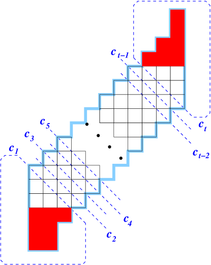
Figure 8: The coordinate filtration for the diagram D𝐷D.
Proof of Theorem 4.

We now compute f(D)𝑓𝐷f(D), where D𝐷D is described in Theorem 4, for the case when m=2k𝑚2𝑘m=2k is even. The case of odd m𝑚m is done similarly and is left to the reader. We choose the usual filtration (C1,C2,,Ct)subscript𝐶1subscript𝐶2subscript𝐶𝑡(C_{1},C_{2},\ldots,C_{t}), except that the first coordinate set C1subscript𝐶1C_{1} represents the tail and the triangular part of the body to which it is attached, and similarly the last coordinate set Ctsubscript𝐶𝑡C_{t} represents the head and the triangular part of the body to which it is attached, as shown in Figure 8. Proposition 12 gives us a good starting position for this computation, since it implies that the first and last transfer operators, T1subscript𝑇1T_{1} and Ttsubscript𝑇𝑡T_{t}, satisfy

(T1𝟏)(x1,,xk)subscript𝑇11subscript𝑥1subscript𝑥𝑘\displaystyle(T_{1}\mathbf{1})(x_{1},\ldots,x_{k}) =\displaystyle= 1i=1kLi!det(xiLj)1i,jk=:ψλ(x1,,xk),\displaystyle\frac{1}{\prod_{i=1}^{k}L_{i}!}\det\bigg{(}x_{i}^{L_{j}}\bigg{)}_{1\leq i,j\leq k}=:\psi_{\lambda}(x_{1},\ldots,x_{k}),
(Tt𝟏)(x1,,xk)superscriptsubscript𝑇𝑡1subscript𝑥1subscript𝑥𝑘\displaystyle(T_{t}^{*}\mathbf{1})(x_{1},\ldots,x_{k}) =\displaystyle= 1i=1kMi!det(xiMj)1i,jk=:ψμ(x1,,xk).\displaystyle\frac{1}{\prod_{i=1}^{k}M_{i}!}\det\bigg{(}x_{i}^{M_{j}}\bigg{)}_{1\leq i,j\leq k}=:\psi_{\mu}(x_{1},\ldots,x_{k}).

The transfer operator for the body part is S2ksubscript𝑆2𝑘S_{2k} defined in (35). Therefore we get using Proposition 8 that

f(D)|D|!=TtS2k2nm+1T1𝟏,𝟏=S2k2n2m+1ψλ,ψμ𝑓𝐷𝐷subscript𝑇𝑡superscriptsubscript𝑆2𝑘2𝑛𝑚1subscript𝑇111superscriptsubscript𝑆2𝑘2𝑛2𝑚1subscript𝜓𝜆subscript𝜓𝜇\frac{f(D)}{|D|!}=\Big{\langle}T_{t}\circ S_{2k}^{2n-m+1}\circ T_{1}\mathbf{1},\mathbf{1}\Big{\rangle}=\Big{\langle}S_{2k}^{2n-2m+1}\psi_{\lambda},\psi_{\mu}\Big{\rangle}

Expanding this using Theorem 10, we get, in the notation of that theorem,

f(D)|D|!=j1>j2>>jk>0λj1,,jk2nm+1ψλ,ϕj1,,jkψμ,ϕj1,,jk.𝑓𝐷𝐷subscriptsubscript𝑗1subscript𝑗2subscript𝑗𝑘0superscriptsubscript𝜆subscript𝑗1subscript𝑗𝑘2𝑛𝑚1subscript𝜓𝜆subscriptitalic-ϕsubscript𝑗1subscript𝑗𝑘subscript𝜓𝜇subscriptitalic-ϕsubscript𝑗1subscript𝑗𝑘\frac{f(D)}{|D|!}=\sum_{j_{1}>j_{2}>\ldots>j_{k}>0}\lambda_{j_{1},\ldots,j_{k}}^{2n-m+1}\Big{\langle}\psi_{\lambda},\phi_{j_{1},\ldots,j_{k}}\Big{\rangle}\Big{\langle}\psi_{\mu},\phi_{j_{1},\ldots,j_{k}}\Big{\rangle}. (40)

To compute ψλ,ϕj1,,jk,ψμ,ϕj1,,jksubscript𝜓𝜆subscriptitalic-ϕsubscript𝑗1subscript𝑗𝑘subscript𝜓𝜇subscriptitalic-ϕsubscript𝑗1subscript𝑗𝑘\Big{\langle}\psi_{\lambda},\phi_{j_{1},\ldots,j_{k}}\Big{\rangle},\Big{\langle}\psi_{\mu},\phi_{j_{1},\ldots,j_{k}}\Big{\rangle}, we use Lemma 13:

ψλ,ϕj1,,jksubscript𝜓𝜆subscriptitalic-ϕsubscript𝑗1subscript𝑗𝑘\Big{\langle}\psi_{\lambda},\phi_{j_{1},\ldots,j_{k}}\Big{\rangle}\qquad\qquad\qquad\qquad\qquad\qquad\qquad\qquad\qquad\qquad\qquad\qquad
=\displaystyle= Ωkdet(xrLsLs!)r,sdet(2cos(π2(2jr1)xs))r,sdx1dxksubscriptsubscriptΩ𝑘subscriptsuperscriptsubscript𝑥𝑟subscript𝐿𝑠subscript𝐿𝑠𝑟𝑠subscript2𝜋22subscript𝑗𝑟1subscript𝑥𝑠𝑟𝑠𝑑subscript𝑥1𝑑subscript𝑥𝑘\displaystyle\int\ldots\int_{\Omega_{k}}\det\bigg{(}\frac{x_{r}^{L_{s}}}{L_{s}!}\bigg{)}_{r,s}\!\!\!\det\bigg{(}\!\!\sqrt{2}\cos\left(\frac{\pi}{2}(2j_{r}-1)x_{s}\right)\!\!\bigg{)}_{r,s}\!dx_{1}\ldots\!dx_{k}
=\displaystyle= 1k![0,1]kdet(xrLsLs!)r,sdet(2cos(π2(2jr1)xs))r,sd𝐱1𝑘subscriptsuperscript01𝑘subscriptsuperscriptsubscript𝑥𝑟subscript𝐿𝑠subscript𝐿𝑠𝑟𝑠subscript2𝜋22subscript𝑗𝑟1subscript𝑥𝑠𝑟𝑠𝑑𝐱\displaystyle\frac{1}{k!}\int\ldots\int_{[0,1]^{k}}\det\bigg{(}\frac{x_{r}^{L_{s}}}{L_{s}!}\bigg{)}_{r,s}\!\!\!\det\bigg{(}\!\!\sqrt{2}\cos\left(\frac{\pi}{2}(2j_{r}-1)x_{s}\right)\!\!\bigg{)}_{r,s}\!d{\bf x}
=\displaystyle= 2k/2det(1Ls!01xLscos(π2(2jr1)x)𝑑x)r,ssuperscript2𝑘2subscript1subscript𝐿𝑠superscriptsubscript01superscript𝑥subscript𝐿𝑠𝜋22subscript𝑗𝑟1𝑥differential-d𝑥𝑟𝑠\displaystyle 2^{k/2}\det\left(\frac{1}{L_{s}!}\int_{0}^{1}x^{L_{s}}\cos\left(\frac{\pi}{2}(2j_{r}-1)x\right)dx\right)_{r,s}
=\displaystyle= 2k/2det(I(Ls,jr))r,s,superscript2𝑘2subscript𝐼subscript𝐿𝑠subscript𝑗𝑟𝑟𝑠\displaystyle 2^{k/2}\det\bigg{(}I(L_{s},j_{r})\bigg{)}_{r,s},

where we have denoted

I(a,j)=1a!01xacos(π2(2j1)x)𝑑x.𝐼𝑎𝑗1𝑎superscriptsubscript01superscript𝑥𝑎𝜋22𝑗1𝑥differential-d𝑥I(a,j)=\frac{1}{a!}\int_{0}^{1}x^{a}\cos\left(\frac{\pi}{2}(2j-1)x\right)dx.

Now, continuing (40), we get, again using Lemma 13 (this time used with a discrete measure), that

(1)(k2)f(D)|D|!superscript1binomial𝑘2𝑓𝐷𝐷(-1)^{\binom{k}{2}}\cdot\frac{f(D)}{|D|!}\qquad\qquad\qquad\qquad\qquad\qquad\qquad\qquad\qquad\qquad\qquad\qquad
=\displaystyle= 2kj1>>jk>0r=1k(2(1)jr+1π(2jr1))2nm+1det(I(Ls,jr))r,sdet(I(Ms,jr))r,ssuperscript2𝑘subscriptsubscript𝑗1subscript𝑗𝑘0superscriptsubscriptproduct𝑟1𝑘superscript2superscript1subscript𝑗𝑟1𝜋2subscript𝑗𝑟12𝑛𝑚1subscript𝐼subscript𝐿𝑠subscript𝑗𝑟𝑟𝑠subscript𝐼subscript𝑀𝑠subscript𝑗𝑟𝑟𝑠\displaystyle\!2^{k}\!\!\!\!\!\!\sum_{j_{1}>\ldots>j_{k}>0}\prod_{r=1}^{k}\left(\frac{2(-1)^{j_{r}+1}}{\pi(2j_{r}-1)}\right)^{2n-m+1}\!\!\!\!\!\!\!\!\!\det\bigg{(}I(L_{s},j_{r})\bigg{)}_{r,s}\!\!\!\!\!\!\det\bigg{(}I(M_{s},j_{r})\bigg{)}_{r,s} (41)
=\displaystyle= 2kk!𝐣kr=1k(2(1)jr+1π(2jr1))2nm+1det(I(Ls,jr))r,sdet(I(Ms,jr))r,ssuperscript2𝑘𝑘subscript𝐣superscript𝑘superscriptsubscriptproduct𝑟1𝑘superscript2superscript1subscript𝑗𝑟1𝜋2subscript𝑗𝑟12𝑛𝑚1subscript𝐼subscript𝐿𝑠subscript𝑗𝑟𝑟𝑠subscript𝐼subscript𝑀𝑠subscript𝑗𝑟𝑟𝑠\displaystyle\frac{2^{k}}{k!}\sum_{{\bf j}\in\mathbb{N}^{k}}\prod_{r=1}^{k}\left(\frac{2(-1)^{j_{r}+1}}{\pi(2j_{r}-1)}\right)^{2n-m+1}\!\!\!\!\!\!\!\!\!\det\bigg{(}I(L_{s},j_{r})\bigg{)}_{r,s}\!\!\!\!\!\!\det\bigg{(}I(M_{s},j_{r})\bigg{)}_{r,s}
=\displaystyle= det(2j=1(2(1)j+1π(2j1))2nm+1I(Ls,j)I(Mr,j))r,s.subscript2superscriptsubscript𝑗1superscript2superscript1𝑗1𝜋2𝑗12𝑛𝑚1𝐼subscript𝐿𝑠𝑗𝐼subscript𝑀𝑟𝑗𝑟𝑠\displaystyle\det\Bigg{(}2\sum_{j=1}^{\infty}\left(\frac{2(-1)^{j+1}}{\pi(2j-1)}\right)^{2n-m+1}I(L_{s},j)I(M_{r},j)\Bigg{)}_{r,s}.

A simple computation, which we include in Appendix A, shows that

I(a,j)𝐼𝑎𝑗\displaystyle I(a,j) =\displaystyle= (1)j+1p=0a/2(1)p(a2p)!(2π(2j1))2p+1superscript1𝑗1superscriptsubscript𝑝0𝑎2superscript1𝑝𝑎2𝑝superscript2𝜋2𝑗12𝑝1\displaystyle(-1)^{j+1}\sum_{p=0}^{\lfloor a/2\rfloor}\frac{(-1)^{p}}{(a-2p)!}\left(\frac{2}{\pi(2j-1)}\right)^{2p+1} (42)
+(1)a+12(2π(2j1))a+11[a odd].superscript1𝑎12superscript2𝜋2𝑗1𝑎1subscript1delimited-[]𝑎 odd\displaystyle+(-1)^{\frac{a+1}{2}}\left(\frac{2}{\pi(2j-1)}\right)^{a+1}1_{[a\text{ odd}]}.

We also verify in Appendix A that

XN(p,q)=2j=1(2(1)j+1π(2j1))NI(p,j)I(q,j).subscript𝑋𝑁𝑝𝑞2superscriptsubscript𝑗1superscript2superscript1𝑗1𝜋2𝑗1𝑁𝐼𝑝𝑗𝐼𝑞𝑗X_{N}(p,q)=2\sum_{j=1}^{\infty}\left(\frac{2(-1)^{j+1}}{\pi(2j-1)}\right)^{N}I(p,j)I(q,j). (43)

Therefore the expression written inside the determinant in (41) is exactly X2nm+1(Ls,Mr)subscript𝑋2𝑛𝑚1subscript𝐿𝑠subscript𝑀𝑟X_{2n-m+1}(L_{s},M_{r}). This proves (10). ∎

Sketch of proof of Theorem 5.

Eq. (14) follows immediately from the case m=2𝑚2m=2 of Theorem 4. Eq. (15) does not follow from Theorem 4, but can be proved using the same techniques. In fact, a both formulas can be treated simultaneously by showing that

XN(p,q)=TN(xp/p!),xq/q!,subscript𝑋𝑁𝑝𝑞superscript𝑇𝑁superscript𝑥𝑝𝑝superscript𝑥𝑞𝑞X_{N}(p,q)=\Big{\langle}T^{N}(x^{p}/p!),x^{q}/q!\Big{\rangle},

where T𝑇T is Elkies’s transfer operator defined in (17), and relating this quantity to αnsubscript𝛼𝑛\alpha_{n} and βnsubscript𝛽𝑛\beta_{n} using Proposition 8 and the trivial (k=1𝑘1k=1) case of Proposition 12. ∎

9 Additional comments and questions

We conclude with some final comments and open questions.

1. More enumeration formulas.

Our treatment of enumeration formulas that can be derived by using the explicit diagonalization of the transfer operators in Theorems 10, 11 is by no means complete and is meant more as an illustration of the power and generality of the technique. One may consider several variant formulas. For example, one may lean the head Young diagram against the vertical side of the triangle (the shape on the right-hand side of Figure 4 is a simple example of this). This will result in enumeration formulas which are minor variations on the formulas of Theorem 4. More generally, one may consider m𝑚m-strip diagrams with head and tail shapes which are not Young diagrams, so that the overall shape is not necessarily even a skew Young diagram. Formula (4) will no longer apply, but the transfer operator technique will still enable deriving enumeration formulas for such “generalized tableaux”, although the use of Proposition 12 would have to be replaced with more tedious manual computation.

2. The principal eigenfunction.

It is interesting to look at the principal eigenfunction of the transfer operators, since, for example, it controls the limiting behavior of uniform random points in the order polytope of a very long m𝑚m-strip diagram (when m𝑚m is fixed and n𝑛n goes to infinity). One gets a simple product representation. For example, for the even case where m=2k𝑚2𝑘m=2k, the principal eigenfunction is

ψ(x1,,xk)=2k/2det(cos(π(2i1)xj2))1i,jk.𝜓subscript𝑥1subscript𝑥𝑘superscript2𝑘2subscript𝜋2𝑖1subscript𝑥𝑗2formulae-sequence1𝑖𝑗𝑘\psi(x_{1},\ldots,x_{k})=2^{k/2}\det\Bigg{(}\cos\left(\frac{\pi(2i-1)x_{j}}{2}\right)\Bigg{)}_{1\leq i,j\leq k}.

By representing each of the cosines as a Chebyshev polynomial in cos(πxj/2)𝜋subscript𝑥𝑗2\cos(\pi x_{j}/2), one can transform this determinant into

ψ(𝐱)=2k/2i=1kcos(πxi2)1i<jk(cos2(πxj2)cos2(πxi2)).𝜓𝐱superscript2𝑘2superscriptsubscriptproduct𝑖1𝑘𝜋subscript𝑥𝑖2subscriptproduct1𝑖𝑗𝑘superscript2𝜋subscript𝑥𝑗2superscript2𝜋subscript𝑥𝑖2\psi({\bf x})=2^{k/2}\prod_{i=1}^{k}\cos\left(\frac{\pi x_{i}}{2}\right)\prod_{1\leq i<j\leq k}\Bigg{(}\cos^{2}\left(\frac{\pi x_{j}}{2}\right)-\cos^{2}\left(\frac{\pi x_{i}}{2}\right)\Bigg{)}.

The probability density ψ(𝐱)2𝜓superscript𝐱2\psi({\bf x})^{2}, which will arise as the stationary distribution of the coordinates of a uniform point in the order polytope when cutting along successive diagonals, is similar to eigenvalue densities arising in random matrix theory. One may hope to exploit this to derive interesting results about random m𝑚m-strip tableaux.

3. Open problem: Generating functions.

It would be interesting to find formulas for the generating functions of some of the families of diagrams treated above. In some cases it’s easy. For example, for the diagram Dnsubscript𝐷𝑛D_{n} in eq. (7) the generating function can be computed to be

n=0f(Dn)x2n(3n)!=x(cotx2cotx).superscriptsubscript𝑛0𝑓subscript𝐷𝑛superscript𝑥2𝑛3𝑛𝑥𝑥2𝑥\sum_{n=0}^{\infty}\frac{f(D_{n})x^{2n}}{(3n)!}=x\left(\cot\frac{x}{2}-\cot x\right).

In more complicated cases we have not found formulas for the generating functions.

4. Open problem: Bijective and combinatorial proofs.

Another direction which might be interesting to pursue is to look for combinatorial or bijective proofs of some of our formulas, for example to prove Theorem 1 by directly relating 333-strip tableaux to up-down permutations in some combinatorial way.

5. Extension to periodic ribbon tableaux.

We restricted our computations to the simplest case of “periodic” Young diagrams, those having the slope (1,1)11(1,1). Most of the results above can be carried over (at the cost of a sizable increase of complexity) to the case of Young diagrams shaped as stacks of m𝑚m periodic ribbon Yound diagrams (if one considers our m𝑚m-strip diagonal YD’s as stacks of m𝑚m up-down YD’s). We plan to present these results in a subsequent publication.

Appendix A. Some computations

A.1. Proof of (42)

Let θ=π2(2j1)𝜃𝜋22𝑗1\theta=\frac{\pi}{2}(2j-1). By repeated integration by parts, we get

I(a,j)𝐼𝑎𝑗\displaystyle I(a,j) =\displaystyle= 1a!01xacos(θx)𝑑x1𝑎superscriptsubscript01superscript𝑥𝑎𝜃𝑥differential-d𝑥\displaystyle\frac{1}{a!}\int_{0}^{1}x^{a}\cos\left(\theta x\right)dx
=\displaystyle= θ1a!xasin(θx)|01+θ2(a1)!xa1cos(θx)|01evaluated-atsuperscript𝜃1𝑎superscript𝑥𝑎𝜃𝑥01evaluated-atsuperscript𝜃2𝑎1superscript𝑥𝑎1𝜃𝑥01\displaystyle\frac{\theta^{-1}}{a!}x^{a}\sin\left(\theta x\right)\big{|}_{0}^{1}+\frac{\theta^{-2}}{(a-1)!}x^{a-1}\cos\left(\theta x\right)\big{|}_{0}^{1}
θ3(a2)!xa2sin(θx)|01θ4(a3)!xa3cos(θx)|01evaluated-atsuperscript𝜃3𝑎2superscript𝑥𝑎2𝜃𝑥01evaluated-atsuperscript𝜃4𝑎3superscript𝑥𝑎3𝜃𝑥01\displaystyle-\frac{\theta^{-3}}{(a-2)!}x^{a-2}\sin(\theta x)\big{|}_{0}^{1}-\frac{\theta^{-4}}{(a-3)!}x^{a-3}\cos(\theta x)\big{|}_{0}^{1}
+θ5(a2)!xa4sin(θx)|01+θ6(a5)!xa5cos(θx)|01evaluated-atsuperscript𝜃5𝑎2superscript𝑥𝑎4𝜃𝑥01evaluated-atsuperscript𝜃6𝑎5superscript𝑥𝑎5𝜃𝑥01\displaystyle+\frac{\theta^{-5}}{(a-2)!}x^{a-4}\sin(\theta x)\big{|}_{0}^{1}+\frac{\theta^{-6}}{(a-5)!}x^{a-5}\cos(\theta x)\big{|}_{0}^{1}
θ7(a6)!xa6sin(θx)|01θ8(a7)!xa7cos(θx)|01+evaluated-atsuperscript𝜃7𝑎6superscript𝑥𝑎6𝜃𝑥01evaluated-atsuperscript𝜃8𝑎7superscript𝑥𝑎7𝜃𝑥01\displaystyle-\frac{\theta^{-7}}{(a-6)!}x^{a-6}\sin(\theta x)\big{|}_{0}^{1}-\frac{\theta^{-8}}{(a-7)!}x^{a-7}\cos(\theta x)\big{|}_{0}^{1}+\ldots
=\displaystyle= (1)j+1p=0a/2(1)p(a2p)!θ(2p+1)+(1)a+12θ(a+1)1[a odd].superscript1𝑗1superscriptsubscript𝑝0𝑎2superscript1𝑝𝑎2𝑝superscript𝜃2𝑝1superscript1𝑎12superscript𝜃𝑎1subscript1delimited-[]𝑎 odd\displaystyle(-1)^{j+1}\sum_{p=0}^{\lfloor a/2\rfloor}\frac{(-1)^{p}}{(a-2p)!}\theta^{-(2p+1)}+(-1)^{\frac{a+1}{2}}\theta^{-(a+1)}1_{[a\text{ odd}]}.

A.2. Proof of (43)

Rewrite (18) as

A¯n=2=1(2(1)+1π(21))n+1.subscript¯𝐴𝑛2superscriptsubscript1superscript2superscript11𝜋21𝑛1\bar{A}_{n}=2\sum_{\ell=1}^{\infty}\left(\frac{2(-1)^{\ell+1}}{\pi(2\ell-1)}\right)^{n+1}.

Using this and (42), the right-hand side of (43) is seen to be

i=0p/2j=0q/2(1)i+j(p2i)!(q2j)![2=1(2(1)+1π(21))N+2i+2j+2]superscriptsubscript𝑖0𝑝2superscriptsubscript𝑗0𝑞2superscript1𝑖𝑗𝑝2𝑖𝑞2𝑗delimited-[]2superscriptsubscript1superscript2superscript11𝜋21𝑁2𝑖2𝑗2\displaystyle\sum_{i=0}^{\lfloor p/2\rfloor}\sum_{j=0}^{\lfloor q/2\rfloor}\frac{(-1)^{i+j}}{(p-2i)!(q-2j)!}\Bigg{[}2\sum_{\ell=1}^{\infty}\left(\frac{2(-1)^{\ell+1}}{\pi(2\ell-1)}\right)^{N+2i+2j+2}\Bigg{]}
+(1)p+12j=0q/2(1)j(q2j)![2=1(2(1)+1π(21))N+p+2j+2]1[p odd]superscript1𝑝12superscriptsubscript𝑗0𝑞2superscript1𝑗𝑞2𝑗delimited-[]2superscriptsubscript1superscript2superscript11𝜋21𝑁𝑝2𝑗2subscript1delimited-[]𝑝 odd\displaystyle+(-1)^{\frac{p+1}{2}}\sum_{j=0}^{\lfloor q/2\rfloor}\frac{(-1)^{j}}{(q-2j)!}\Bigg{[}2\sum_{\ell=1}^{\infty}\left(\frac{2(-1)^{\ell+1}}{\pi(2\ell-1)}\right)^{N+p+2j+2}\Bigg{]}1_{[p\text{ odd}]}
+(1)q+12i=0p/2(1)i(p2i)![2=1(2(1)+1π(21))N+2i+q+2]1[q odd]superscript1𝑞12superscriptsubscript𝑖0𝑝2superscript1𝑖𝑝2𝑖delimited-[]2superscriptsubscript1superscript2superscript11𝜋21𝑁2𝑖𝑞2subscript1delimited-[]𝑞 odd\displaystyle+(-1)^{\frac{q+1}{2}}\sum_{i=0}^{\lfloor p/2\rfloor}\frac{(-1)^{i}}{(p-2i)!}\Bigg{[}2\sum_{\ell=1}^{\infty}\left(\frac{2(-1)^{\ell+1}}{\pi(2\ell-1)}\right)^{N+2i+q+2}\Bigg{]}1_{[q\text{ odd}]}
+(1)p+q2+1[2=1(2(1)+1π(21))N+p+q+2]1[p,q odd]superscript1𝑝𝑞21delimited-[]2superscriptsubscript1superscript2superscript11𝜋21𝑁𝑝𝑞2subscript1𝑝𝑞 odd\displaystyle+(-1)^{\frac{p+q}{2}+1}\Bigg{[}2\sum_{\ell=1}^{\infty}\left(\frac{2(-1)^{\ell+1}}{\pi(2\ell-1)}\right)^{N+p+q+2}\Bigg{]}1_{[p,q\text{ odd}]}
=\displaystyle= i=0p/2j=0q/2(1)i+jA¯N+2i+2j+1(p2i)!(q2j)!superscriptsubscript𝑖0𝑝2superscriptsubscript𝑗0𝑞2superscript1𝑖𝑗subscript¯𝐴𝑁2𝑖2𝑗1𝑝2𝑖𝑞2𝑗\displaystyle\sum_{i=0}^{\lfloor p/2\rfloor}\sum_{j=0}^{\lfloor q/2\rfloor}\frac{(-1)^{i+j}\bar{A}_{N+2i+2j+1}}{(p-2i)!(q-2j)!}
+(1)p+12j=0q/2(1)jA¯N+p+2j+1(q2j)!1[p odd]superscript1𝑝12superscriptsubscript𝑗0𝑞2superscript1𝑗subscript¯𝐴𝑁𝑝2𝑗1𝑞2𝑗subscript1delimited-[]𝑝 odd\displaystyle+(-1)^{\frac{p+1}{2}}\sum_{j=0}^{\lfloor q/2\rfloor}\frac{(-1)^{j}\bar{A}_{N+p+2j+1}}{(q-2j)!}1_{[p\text{ odd}]}
+(1)q+12i=0p/2(1)iA¯N+q+2i+1(p2i)!1[q odd]superscript1𝑞12superscriptsubscript𝑖0𝑝2superscript1𝑖subscript¯𝐴𝑁𝑞2𝑖1𝑝2𝑖subscript1delimited-[]𝑞 odd\displaystyle+(-1)^{\frac{q+1}{2}}\sum_{i=0}^{\lfloor p/2\rfloor}\frac{(-1)^{i}\bar{A}_{N+q+2i+1}}{(p-2i)!}1_{[q\text{ odd}]}
+(1)p+q2+1A¯N+p+q+11[p,q odd]superscript1𝑝𝑞21subscript¯𝐴𝑁𝑝𝑞1subscript1𝑝𝑞 odd\displaystyle+(-1)^{\frac{p+q}{2}+1}\bar{A}_{N+p+q+1}1_{[p,q\text{ odd}]}
=\displaystyle= XN(p,q).subscript𝑋𝑁𝑝𝑞\displaystyle X_{N}(p,q).

References

  • [1] A. C. Aitken. The monomial expansion of determinantal symmetric functions. Proc. Royal Soc. Edinburgh (A) 61 (1943), 300–310.
  • [2] D. André. Developpements de secx𝑥\sec x et de tang xtang 𝑥\text{tang }x. Comptes Rendus Acad. Sci. Paris 88 (1879), 965–967.
  • [3] D. André. Mèmoire sur les permutations alternées J. Math. 7 (1881), 167–184.
  • [4] C. Andréief, Note sur une relation pour les intégrales définies des produits des fonctions, Mém. Soc. Sci. Bordeaux 2 (1881), 1­-14.
  • [5] V. I. Arnold. Bernoulli-Euler updown numbers associated with function singularities, Duke math. J. 63 (1991), 537–555.
  • [6] Yu. Baryshnikov. GUEs and queues. Probab. Theory and Rel. Fields 119 (2001), 256–274/
  • [7] R. J. Baxter. Exactly Solved Models in Statistical Mechanics. Academic Press, New York, 1982.
  • [8] C. Boutillier. Preprint,
    http://www.arxiv.org/abs/math/0607162.
  • [9] J.M. Borwein, P.B. Borwein, K. Dilcher. Pi, Euler numbers and asymptotic expansions. Amer. Math. Monthly 96 (1989), 681–687.
  • [10] N. Elkies. On the sums k=(4k+1)nsuperscriptsubscript𝑘superscript4𝑘1𝑛\sum_{k=-\infty}^{\infty}(4k+1)^{-n}. Amer. Math. Monthly 110 (2003), 561–573.
  • [11] N. Elkies, G. Kuperberg, M. Larsen, J. Propp. Alternating-sign matrices and domino tilings. J. Algebraic Combin. 1 (1992), 111–132, 219–234.
  • [12] W. Feit. The degree formula for the skew-representations of the symmetric group. Proc. Amer. Math. Soc. 4 (1953), 740–744.
  • [13] D. E. Knuth. The Art of Computer Programming, Vol. 3: Sorting and Searching, Second Edition. Addison-Wesley, Reading, MA, 1998.
  • [14] J. Millar, N. J. A. Sloane, N. E. Young. A new operation on sequences: the boustrophedon transform. J. Combin. Th. Sr. A 76 (1996), 44–54.
  • [15] R. P. Stanley. Enumerative Combinatorics, Vol. 2. Cambridge University Press, Cambridge, 1999.