Predictive protocol of flocks with small-world connection pattern

Abstract

By introducing a predictive mechanism with small-world connections, we propose a new motion protocol for self-driven flocks. The small-world connections are implemented by randomly adding long-range interactions from the leader to a few distant agents, namely pseudo-leaders. The leader can directly affect the pseudo-leaders, thereby influencing all the other agents through them efficiently. Moreover, these pseudo-leaders are able to predict the leader’s motion several steps ahead and use this information in decision making towards coherent flocking with more stable formation. It is shown that drastic improvement can be achieved in terms of both the consensus performance and the communication cost. From the industrial engineering point of view, the current protocol allows for a significant improvement in the cohesion and rigidity of the formation at a fairly low cost of adding a few long-range links embedded with predictive capabilities. Significantly, this work uncovers an important feature of flocks that predictive capability and long-range links can compensate for the insufficiency of each other. These conclusions are valid for both the attractive/repulsive swarm model and the Vicsek model.

I Introduction

Over the last decade, physicists have been looking for common, possibly universal, features of the collective behaviors of animals, bacteria, cells, molecular motors, as well as driven granular objects. The collective motion of a group of autonomous agents (or particles) is currently a subject of intensive research that has potential applications in biology, physics and engineering. One of the most remarkable characteristics of systems, such as flocks of birds, schools of fish, and swarms of locusts, is the emergence of collective states in which the agents move in the same direction, i.e., an ordered state vi95 ; do06 ; ch06 ; he05 ; gr04 ; al07 ; li08 . Moreover, this ordered state seeking problem for flocks/swarms/schools can be further generalized to consensus sa04 , rendezvous, synchrony, cooperation and so on. From the application aspect, this kind of distributed collective dynamic systems has direct implications on sensor network data fusion, load balancing, unmanned air vehicles (UAVs), attitude alignment of satellite clusters, congestion control of communication networks, multi-agent formation control and global coordination for emergency ak02 ; og04 ; ar02 ; he00 .

The interaction pattern of the natural biological flocks/swarms are neither entirely regular nor entirely random. An individual of a flock usually knows its neighbors, but its circle of acquaintances may not be confined to those who live right next door. In 1998, in order to describe the transition from a regular lattice to a random graph, Watts and Strogatz (WS) introduced the concept of the small-world network wa98 by rewiring one end of a few connections to new nodes chosen at random from the whole network. With these few shortcuts, the average distance is decreased significantly without crucially changing the clustering property. The work on the WS small-world network has started an avalanche of research on complex networks, especially, the synchronizability of networks can be greatly enhanced by introducing a few long-range connections wa03 ; zh06 ; al03 . Thus, for better synchronization in a flock of neighboring-connected agents with a leader, it is advantageous to build a small-world-type network structure by randomly adding long-range connections from the leader to a few distant agents (namely pseudo-leaders), so that the leader can affect them, thereby influencing all the other agents through them, via fast communication and rapid control commands.

Although a lot of relevant works were focused on network structures, recently, more and more researchers are interested in finding the rules of the inter-connections present in abundant bio-groups. Extraction of these rules can help interpret why the bio-groups can demonstrate so many good characteristics such as synchronization, stabilisation, cohesion, etc. A fairly basic but popular flocking strategy can be traced back to the Reynolds Model re87 , in which three elementary flocking protocols are prescribed, (i) separation: steer to avoid crowding and collision; (ii) alignment: steer towards the average heading; (iii) cohesion: steer to move towards the average position. These rules have been proven to be effective and thus become the basic rules for the design of bio-group dynamic models. In 2003, Gazi and Passino ga03 proposed an effective A/R (attractive/repulsive) swarm model in which the motion of each individual (autonomous agent or biological creature) is determined by two factors: (i) attraction to the other individuals on long distances; (ii) repulsion from the other individuals on short distances.

The Gazi and Passino A/R model ga03 , embedded with a similar mechanism of the inter-molecular force, is derived from the biological flocks/swarms behaviors. Thus far, the general understanding is that the swarming behaviors result from an interplay between a long-range attraction and a short-range repulsion between the individuals br54 ; wa91 . In br54 , Breder suggested a simple model composed of a constant attraction term and a repulsion term which is inversely proportional to the square of the distance between two members, whereas in wa91 Warburton and Lazarus studied the effects on cohesion of a family of attraction/repulsion functions. Moreover, in physics communiuty, a large volume of literature on systems with interactive particles have also adopted functions of attractive and repulsive forces to investigate the dynamics of the system le98 ; be90 ; we98 ; ar07 ; sc92 ; me99 ; oh93 . For instance, in le98 ; be90 , systems of particles interacting in a lattice are considered with attraction between particles located at different sites and repulsion between particles occupying the same site. It is discussed in we98 that, the structure of a nonuniform Lennard-Jones (LJ) liquid near a hard wall is approximated by that of a reference fluid with repulsive intermolecular forces in a self-consistently determined external mean field incorporating the effects of attractive forces.

With the A/R model ga03 , Gazi and Passino proved that the individuals will form a bounded cohesive swarm in a finite time. One year later, by adding another factor, i.e., attraction to the more favorable regions (or repulsion from the unfavorable regions), they generalized their former model into a social foraging swarm model ga04 . Under some suitable circumstance, agents in this modified model are apt to move to the more favorable regions. The A/R model has been adopted by physicists and biologists to model self-driven particles and biological flocks sh06 ; zi07 ; do06 ; ch07 ; li07a ; li07b . In 2004, Moreau mo04 presented a linearized model of flocks, and proved that the flock is uniformly and globally cohesive to a bounded circle if and only if there exists an agent (the “leader”) connecting to all other agents, directly or indirectly, over an arbitrary time interval. Other than these kinds of A/R models ga03 ; ga04 ; mo04 , another popular kind of model is that without leaders (say homogeneous), where a very representative one is the Vicsek Model vi95 . In each step, every agent updates its velocity according to the average direction of its neighbors. With the decrease of external noise or the increase of the particle density, the collective behavior of the flock undergoes a phase transition from the randomly distributed phase to the coherently moving phase. In 2003, Jadbabaie et al. provided the convergence condition of the noise-free Vicsek model, i.e., the individuals are linked in some intervals ja03 .

Figure 1: (Color online) Predictive vision in natural bio-groups. Each individual makes its motion decision based on not only the current status of the leader and its neighbors but also their future dynamics.

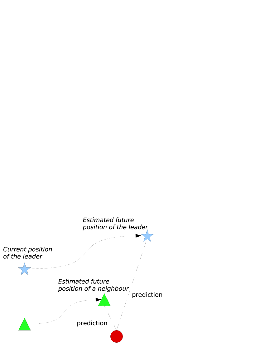
Although most of the previous works on flock dynamics yield many advantages such as synchronization, stabilization, cohesion, and quick consensus, agents within the networks only know the information that is currently available to them. In this paper, we highlight another appealing phenomenon, i.e. the universal existence of predictive mechanism in various biological aggregated systems. A general physical picture behind this is illustrated in Fig. 1 and interpreted as follows: in widely-spread natural bio-groups composed of animals, bacteria, cells, etc., the decision on the next-step behavior of each individual is not solely based on the currently available state information (including position, velocity, etc.) of other (neighboring) agents inside the group but also on the predictions of future states. More precisely, taking a few past states of its leader and neighbors into account, an individual can estimate the corresponding future states several steps ahead and then make a decision.

Some experimental evidences have already been reported in the literature. In 1959, Woods implemented some experiments on bee swarms and found a certain predictive mechanism of electronic signals inside this bio-group wo59 . Also for bee swarms, in 2002, Montague et al. discovered that there exist some predictive protocols in the foraging process in uncertain environments mo00 . Apart from the investigation of the predictive mechanisms of locust swarming and foraging, more scholars focused on the predictive function of the optical and acoustical apparatuses of the individuals inside bio-groups go03 ; su06 ; me07 , especially cortexes and retinae. For instance, based on intensive experiments on the bio-eyesight systems, they found that when an individual observer prepared to follow a displacement of the stimulus with the eyes, visual form adaptation was transferred from current fixation to the future gaze position. These investigations strongly support our conjecture of the existence of some predictive mechanisms inside abundant bio-groups.

Bearing in mind the plentiful examples of predictive protocols inside natural bio-groups, we incorporated some predictive functions into a few long-range links, and found that it is possible to significantly enhance the flocking performances at a fairly low cost of the additional predictive energy. More interestingly, proper prediction capability can help reduce the minimal number of the long-range links between the leader and the pseudo-leaders, thus effectively decrease the communication cost.

On the other hand, from the industrial application point of view, the phenomena and strategy reported in this paper may be applicable in some relevant prevailing engineering areas like autonomous robot formations, sensor networks and UAVs ak02 ; og04 ; ar02 . Typically, due to the limitation of the communication energy, only a few agents have the capability to communicate with the leader. The incorporation of a predictive mechanism into these pseudo-leaders can greatly improve the flocking performances.

The rest of this paper is organized as follows. In Section II, the small-world connection model with embedded predictive mechanism is presented. Then, in Section III, its important role in improving flocking synchronization performances is extracted and analyzed by numerical simulations on the A/R model ga03 . Afterwards, in Section IV, the generality of the virtues endowed by such predictive mechanism is validated on the Vicsek model vi95 as well. Finally, conclusions are drawn in Section V.

II Model

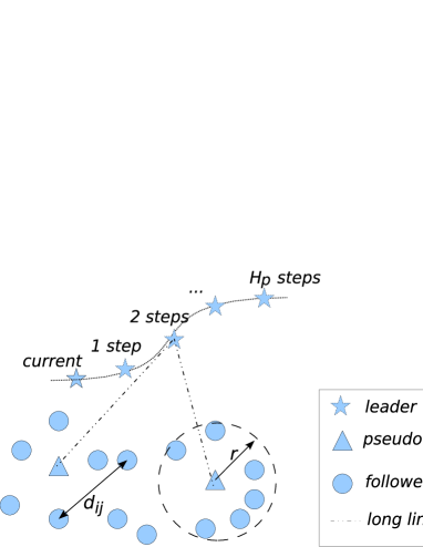
It is well-known that a ring-shaped network structure is not a good one for efficient mutual communication and global control within a flock of agents, while the so-called small-world networking structure performs much better. By adding a few long-range connections, the average path length of the ring-shaped network will be abruptly decreased. This small-world effect is very desirable for fast communication and information transmission, efficient synchronization, and effective global control over the entire network zh06 . Thus, in a flock of neighboring-connected agents with a leader, for communication and control purposes, it is advantageous to build a small-world-type network by randomly adding long-range connections from the leader to a few distant agents (namely pseudo-leaders). As shown in Fig. 2, the leader can affect pseudo-leaders, thereby influencing all the other agents through them. To be clear, we call the non-special agents followers. Thus in our model, there are three different kinds of agents: leader (L), pseudo-leaders (P), and followers (F).

Figure 2: Small-world predictive mechanism of flocks. Here, the leader (L), pseudo-leaders (P), and followers (F) are denoted by star, triangles and circles, respectively, and the neighboring area of each individual is a circle with radius $r$ centering at itself. The leader’s trajectory is given in advance, which will not influenced by the others. Each pseudo-leader’s dynamics is always influenced by both the leader’s future position $H_{p}$ steps ahead and its neighbors’ positions, while each follower’s dynamics is solely affected by its neighbors’ positions.

Figure 3: (Color online) Information communication process inside flocks with a predictive mechanism. The arrows represent the passing of position information. If the pseudo-leader $i$ predicts the dynamics of the leader $H_{p}$ steps ahead, then the follower $j$, within topological distance equaling $H_{p}$ from $i$, could be affected by the current location of the leader. Here, an agent $j$ has topological distance zero to itself, and 1 to all the agents located inside the circle with radius $r$ centered on $j$. Two agents having topological distance 1 are called connected. An agent has topological distance $D_{T}$ to $j$ if and only if it is connected to at least one agent with distance $D_{T}-1$ to $j$, while is not connected with any agents having distance smaller than $D_{T}-1$ to $j$. Note that all the agents are not necessarily embedded in a circular pathway. Instead, due to the circle-shaped neighborhood of each agent, the position information transmission pathway forms a tube tangent to these neighboring circles, and the layout boundary of the pathway could be any types of curves depending on the location of the agents.

In this model, the flock is assumed to move in an $m$-dimensional space and the standard A/R function sa04 ; ga03 ; ga04

$$G(d_{pL})=-d_{pL}\left(a-b\cdot\mbox{exp}(-\|d_{pL}\|_{2}^{2}/c)\right)$$ (1)

is used as long-range interaction from the leader (L) to each pseudo-leader (P), where $a$, $b$, $c$ are three free parameters, $d_{pL}$ is the $m$-dimensional vector pointing from the predicted location of leader $L$ to the current location of a pseudo-leader $p$, and $\|d_{pL}\|_{2}=\sqrt{d_{pL}^{T}d_{pL}}$ denotes the Euclidean distance between them. The force $G(d_{pL})$ is an $m$-dimensional vector whose direction is from the pseudo-leader to the leader. For simplicity, in our model, the motion of leader is given in advance, and will not be affected by any other agents. We assume every pseudo-leader has the same prediction horizon $H_{p}$, that is to say, a pseudo-leader will predict the leader’s location $H_{p}$ steps ahead.

On the other hand, a weaker A/R function, representing the short-range interaction between two arbitrary neighboring agents $i$ and $j$ is addressed as:

$$g(d_{ij})=-d_{ij}\left(\tilde{a}-\tilde{b}\cdot\mbox{exp}(-\|d_{ij}\|_{2}^{2}/\tilde{c})\right),$$ (2)

where $d_{ij}$ is the $m$-dimensional vector pointing from the individuals $j$ to $i$, and $\|d_{ij}\|_{2}=\sqrt{d_{ij}^{T}d_{ij}}$ denotes the Euclidean distance between them. The parameters $\tilde{a}$, $\tilde{b}$ and $\tilde{c}$ are much smaller than $a$, $b$, and $c$, respectively. The direction of vector $g(d_{ij})$ is from $i$ to $j$. Denote by $r$ the radius of neighboring area (see Fig. 2). The neighboring A/R links could connect any two agents (F-F, P-P and L-F) within the Euclidean distance $r$ except the L-P interaction described in Eq. (1). Note that the leader can influence other agents, but will not be influenced. In order to decrease the prediction cost, no predictive mechanism is incorporated into the neighboring A/R links. Bearing in mind the physical meaning of A/R function sa04 , the positions of a pseudo-leader $z_{p}$ and a follower $z_{i}$ (both $z_{p}$ and $z_{i}$ are $m$-dimensional vectors) are determined by

$$\dot{z}_{p}(t)=\underbrace{G(d_{pL}(t+H_{p}))}_{long~{}link~{}to~{}the~{}leader}+\underbrace{\sum_{j\neq L,d_{pj}(t)\leq r}g(d_{pj}(t)),}_{neighboring~{}links}$$ (3)

and

$$\dot{z}_{i}(t)=\underbrace{\sum_{j,d_{ij}(t)\leq r}g(d_{ij}(t)),}_{neighboring~{}links}$$ (4)

respectively, where $t$ denotes the current time, and $d_{pL}(t+H_{p})$ represents the $m$-dimensional vector pointing from the leader’s position $H_{p}$ steps ahead to the current position of a pseudo-leader. Although the rest of this paper concentrates on the motions in $2$-dimensional space, the present model can be directly applied in any finite dimensional space. In this way, unlike the routine flocking strategies mo04 ; ga03 ; ga04 ; co05 , a small-world interaction pattern is established with embedded predictive mechanism, which has the capability of predicting the future behavior (position, velocity, etc.) of the leader several steps ahead. Note that the structure of this interaction network will change in time since the location of each agent is varying.

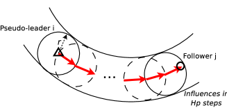
The information communication process is illustrated in Fig. 3. The farthest agent $i_{1}$ directly communicating with agent $i$ is among the ones at the rim of the circle with radius $r$ centered on agent $i$. Analogously, the farthest agent $i_{2}$ directly influenced by $i_{1}$ is also located at the rim of the circle centered on agent $i_{1}$, and so forth. Finally, the influence of agent $i$ reaches agent $j$ in $H_{p}$ steps. When agent $j$ receives the information from agent $i$ at time $t$, it is in fact a delayed information of agent $i$ at time step $t-H_{p}$. However, if agent $i$ acts as a pseudo-leader who can accurately predict the behavior of the leader $H_{p}$ steps ahead, then, at time step $t$, agent $j$’s motion is affected by the exact current location of the leader $z_{L}(t)$. In this way, although agent $j$ may not have direct connection with the leader, it could know some information of the leader’s current dynamics by agent $i$’s delayed information. Therefore, agent $j$ can adhere to the leader more tightly, the flock’s formation is more likely to be stable, and the coherence of the whole flock is thus improved effectively. Note that, the predictive mechanism is valid only if the leader’s motion is regular ex1 . If the leader moves in some random, chaotic or other irregular ways, such as random walk, it is, in principle, impossible for the pseudo-leaders to predict the leader’s further location. Fortunately, in the real biological world, the flock leader always moves in some predictable pattern. Therefore, the other agents have the opportunity to display their predicting ability, such as that used by a chameleon to capture a fly and by a dog to catch a frisbee.

III Analysis and simulations

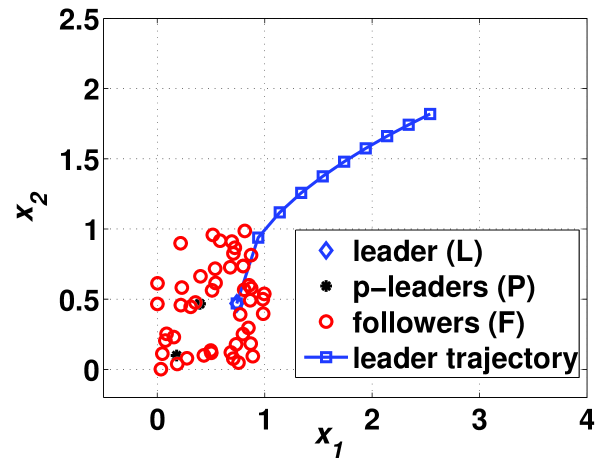
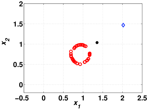
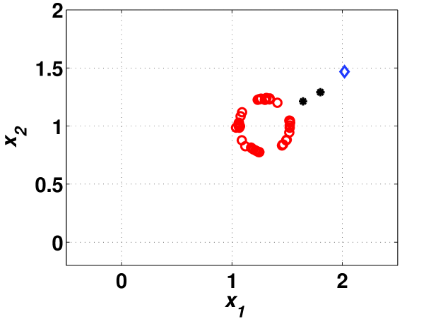
To show the advantages of the predictive mechanism, we compare the performances of the two cases of flocking with and without the predictive mechanism by simulations over an $N$-agent flock moving in a two-dimensional space as shown in Fig. 4. The parameters are set as follows: the neighboring circle $r=0.65$, the parameters of the A/R functions (see Eqs. (1) and (2)) of long-range links and neighboring links are set as $a=8$, $b=17.6$, $c=3.2$, and $\tilde{a}=1$, $\tilde{b}=2.2$, $\tilde{c}=0.2$, respectively. The former A/R function is much stronger in order to intensify the influence of the leader. As shown in Fig. 4a, each agent starts from a position randomly selected in the square $[0,1]\times[0,1]$. The leader and the pseudo-leaders are selected randomly among these $N$ agents. The trajectory of the leader is set as $x_{2}=\sqrt{x_{1}}$, and the velocity of the leader is $v_{L_{x_{1}}}(t)=0.02,~{}v_{L_{x_{2}}}(t)=\sqrt{0.02(t+1)}-\sqrt{0.02t}$. In our simulations, the time label $t$ is a discrete number with step length being equal to $1$.

(a)	(b)
(c)	(d)

Figure 4: (Color online) (a) Starting position of the 50-agent flock consisting of 1 leader, 2 pseudo-leaders and 47 followers. The blue line marked by square points denotes the trajectory of the leader. (b) Flock position after 65 steps without predictive mechanism ($H_{p}=0$), (c) with proper predictive mechanism ($H_{p}=20$), and (d) with over prediction ($H_{p}=70$). Here, $x_{1}$ and $x_{2}$ denote the two-dimensional position coordinates.

(a)	(b)
(c)	(d)

Figure 5: (Color online) The roles of the pseudo-leaders’ number $N_{pl}$ (figures (a) and (c)) and prediction horizon $H_{p}$ (figures (b) and (d)) on a flock of $50$ agents. The leader and the pseudo-leaders are selected randomly among these agents. Each point is an average over $1000$ independent runs. The parameters of the A/R functions (1) and (2) are $a=8$, $b=17.6$, $c=0.4$, and $\tilde{a}=1$, $\tilde{b}=2.2$, $\tilde{c}=0.2$, respectively. The radius of the influence circle is $r=0.65$. Each agent starts from a position randomly selected in the square $[0,1]\times[0,1]$. Without loss of generality, the trajectory of the leader is set along the curve defined by $x_{2}=\sqrt{x_{1}}$, and the velocity of the leader is $v_{L_{x_{1}}}(t)=0.02,~{}v_{L_{x_{2}}}(t)=\sqrt{0.02(t+1)}-\sqrt{0.02t}$.

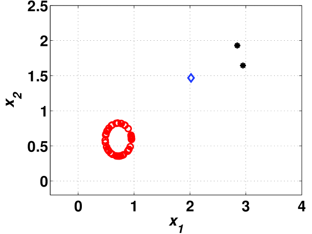
It can be seen from Figs. 4b–4d that, with a proper $H_{p}$, the coherence of the flock will be improved remarkably. The followers will adhere to the leader much more tightly (see Fig. 4c), and the flock formation will be more stable. More precisely, for the flocks with the predictive mechanism, the position error index

$$J_{p}=\frac{1}{N-1}\sum_{i=1,i\neq L}^{N}\|d_{iL}\|_{2}$$ (5)

converges to a constant after finite steps, indicating a stable state of the flock dynamics. Here, $J_{p}$ measures the cohesion performance of the flock, with $\|d_{iL}\|_{2}$ denoting the Euclidean distance between agent $i$ (F or P) and the leader. Meanwhile, as to the flock without this mechanism, as shown in Fig. 4b, $J_{p}$ will keep increasing along with the elapse of time, making the flocking unstable. However, abusing the foresight, namely over-prediction (see Fig. 4d), is also undesirable. That is because the pseudo-leaders are attracted/repelled by the leader position too many steps ahead and will probably escape the flock with a fairly high speed, and then lose influences on the followers. In this way, the flocking will be damaged after finite steps.

The circular formation of the followers in Figs. 4b–4d is because of the particular form of the A/R function. To be clear, we give a more detailed explanation as follows: Actually, the biological flock dynamics is fairly complex. For example, fish uses sidetrack to sense the current variances, in this way, the fish schools are formed. On the other hand, in order to save flying energy for the rear individuals, wild geese flocks always form a ‘$\Lambda$’-like formation kr02 . In this case, the forming process of such flock is determined by aerodynamics. Our proposed model is based on the idea that an individual inside a bio-group can predict the trajectory of its leader(s), and this kind of intelligence can help the individual make more efficient decision to improve the flocking performance. This paper, however, does not aim at reproducing the detailed movement formations of any particular bio-groups.

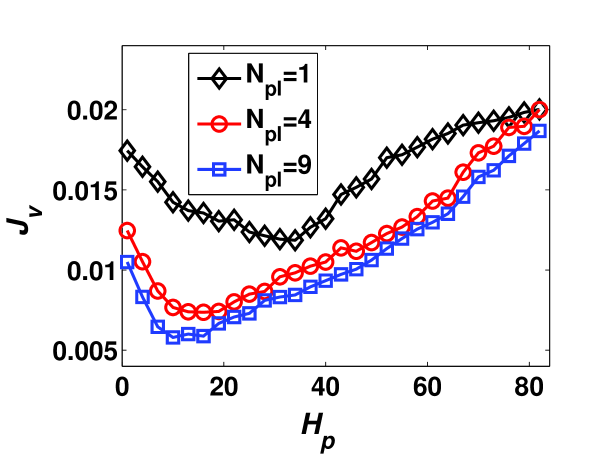
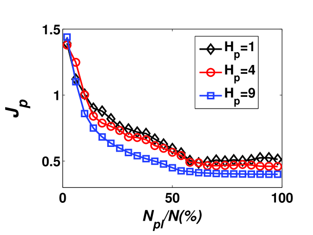
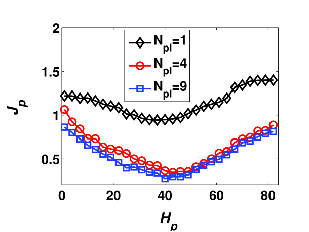
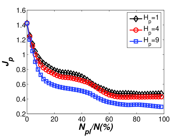
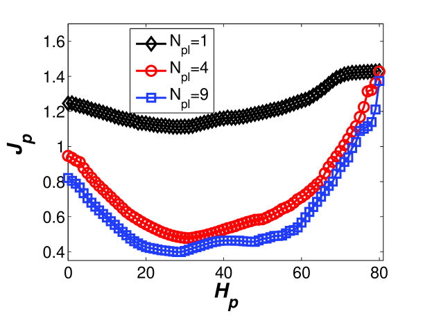
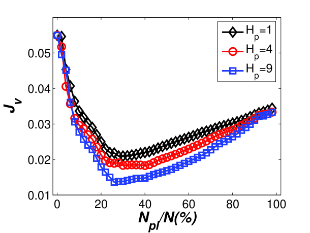
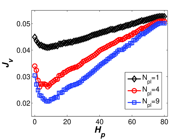
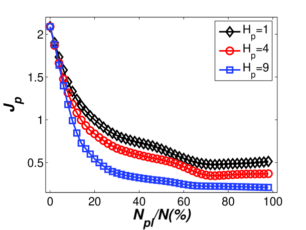
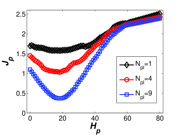
In order to extract the role of $H_{p}$ and the number of pseudo-leaders denoted by $N_{pl}$, we display their influences on the position error index $J_{p}$ and velocity error index $J_{v}$ in Fig. 5, where

$$J_{v}=\frac{1}{N-1}\sum_{i=1,i\neq L}^{N}\|\overrightarrow{v_{i}}-\overrightarrow{v_{L}}\|_{2}.$$ (6)

Here, $J_{v}$ measures the formation performance of the flock, where $\overrightarrow{v_{L}}$ and $\overrightarrow{v_{i}}$ denote the velocity vectors of the leader and the $i$th agent (F or P). If $J_{v}\rightarrow 0$, the relative velocity of each pair of agents approaches zero, thus the flock formation is fixed. In Fig. 5a, we fix $H_{p}$ and display the curves of $J_{v}$ with increasing $N_{pl}$, while Fig. 5b, on the contrary, reports the curves of $J_{v}$ with increasing $H_{p}$ and fixed $N_{pl}$. It can be seen from Fig. 5a that the curves fall sharply at the beginning and then more slowly until reaching a minimum, afterwards rising slowly as the increasing of $N_{pl}$. It implies that adding just very few pseudo-leaders (e.g. long-range links) to the leader, which transforms the flock topology from a strongly localized network into a small-world one, will improve the flocking performance greatly. However, when the number of pseudo-leaders reaches an optimum $N_{pl}^{*}$ corresponding to the minimal $J_{v}^{*}$, the flock formation performance will start to worsen and these extra pseudo-leaders become redundant. On the other hand, increasing $H_{p}$ can help reduce $J_{v}$ in two ways: (i) it depresses $J_{v}$ with the same $N_{pl}$; (ii) it reduces the optimal value of $N_{pl}^{*}$ corresponding to the minimal $J_{v}^{*}$. Compared with Fig. 5a, the $J_{v}$ curves in Fig. 5b fall more slowly at the beginning until reaching the minimum, afterwards $J_{v}$ increases all along and never reaching a stable platform. It implies that the flock formation performance can be remarkably improved with proper predictive capability, however, too much vision into the future, namely over-prediction, will even worsen the formation of flocking. On the other hand, more pseudo-leaders, i.e., larger $N_{pl}$ (as long as $N_{pl}\leq N_{pl}^{*}$), can also help yield more cohesive flocking with better formation.

Figure 6: (Color online) Illustration of Fig. 5a. Follower C heads in the red dashed arrow direction with the guide of pseudo-leader A who moves nearly in the same direction as the leader, making the movement direction nearly synchronized. However, the addition of pseudo-leader B will make the direction of C deviate from the red dashed arrow to the green arrow, and thus worsen the velocity synchronization performance $J_{v}$. Therefore, more pseudo-leaders are not necessarily beneficial to synchronizing the velocities of the flock.

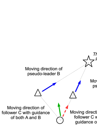
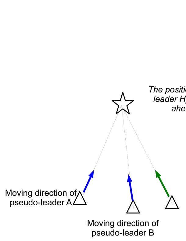
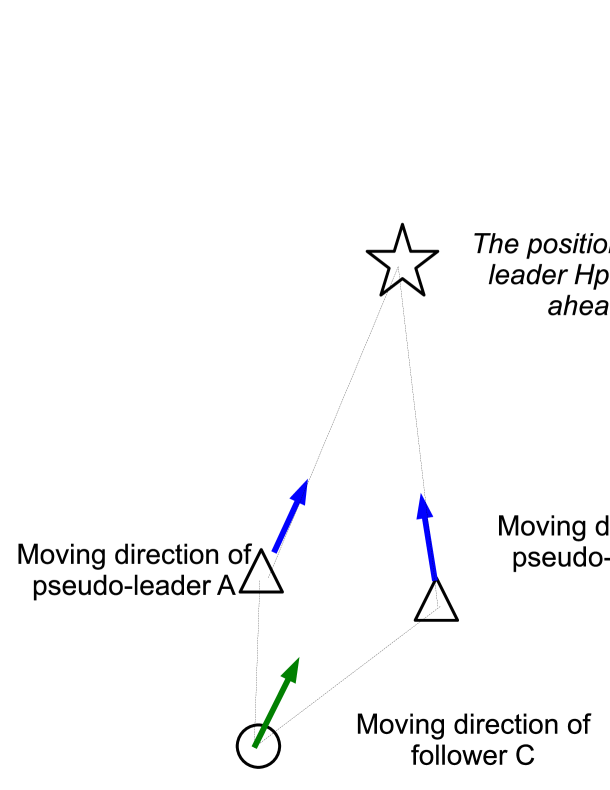
An interesting phenomenon can be observed from Fig. 5a that increasing the number of pseudo-leaders beyond some characteristic number makes the flocking performance worse, which seems counter-intuitive. This can be explained as follows. First, as shown in Eqs. (3) and (4), the velocities of both the pseudo-leaders and the followers are solely determined by the relative positions. Indeed, as shown in Fig. 6, if there is only one pseudo-leader A, then the follower C will head in the red dashed arrow towards A, and all the three individuals are nearly moving in the same direction, which is desirable. However, when another pseudo-leader B is added into this flock, the follower C will move towards a certain position between A and B (see the green arrow). Apparently, the velocity synchronization performance is worsened compared with the former case. Therefore, the observation in Fig. 5a is reasonable. To give a more vivid and detailed explanation, we give further discussions in Appendix A for interested readers.

Next, we investigate the effects of $H_{p}$ and $N_{pl}$ for another important index $J_{p}$. It can be seen from Fig. 5c that the curves fall sharply at the beginning and then asymptotically approach a stable value. The main difference between Fig. 5a and Fig. 5c is that the latter is monotonous and has no minimum, in other words, the increase of $N_{pl}$ always improves $J_{p}$. A special case explaining this phenomenon is that if all the followers serve as the pseudo-leaders, then they will be very cohesive to the leader. However, when $N_{pl}$ exceeds a certain value $\bar{N}_{pl}$, $J_{p}$ will increase so slowly that almost no substantial improvement can be achieved. Moreover, increasing $H_{p}$ can help reduce $J_{p}$, and the improvement shrinks along with increasing $H_{p}$, indicating a saturation effect that no remarkable improvement can be achieved by pushing $H_{p}$ to a very high value (which may cost too much). Compared with Fig. 5c, the curves of Fig. 5d decrease more slowly first and then reach the lowest values at a fairly large $H_{p}$, afterwards rise quickly. Thus, over-prediction is not preferred. Analogous to Fig. 5b, more pseudo-leaders will help improve the cohesive flocking performance, however, this improvement also displays a saturation effect with increasing $N_{pl}$. Actually, when $N_{pl}$ exceeds a certain value, $J_{p}$ increases very slowly that almost no benefit can be gained by further increasing $N_{pl}$. In brief, suitable insight into the future and moderate number of pseudo-leaders are preferred.

A plausible physical rule behind the observed phenomena shown in Fig. 5 is that, in order to achieve a fixed flocking performance, greater predictive capability and more pseudo-leaders can compensate the insufficiency of each other. Given a fixed-size flock, separately for formation performance $J_{v}$ and cohesive performance $J_{p}$, there exists an optimized combination of $H_{p}$ and $N_{pl}$. The conclusions achieved in this paper are not sensitive to the trajectory of the leader. In order to validate the generality of the conclusions, we have used another two different trajectories, i.e., parabolic and sinusoidal curves. The simulation results are shown in Appendix B, which suggest that our main conclusion, i.e., predictive capability and long-range links can compensate for the insufficiency of each other, also holds in those two cases.

(a)	(b)

Figure 7: (Color online) With-noise case vs. noise-free case for a flock with $N=50$, $N_{pl}=9$, and $\eta=0.02$. The other parameters and the initial conditions are the same as those in Fig. 5. Each point is an average over 1000 independent runs. The moderate external noise does not change the global behavior of the flock.

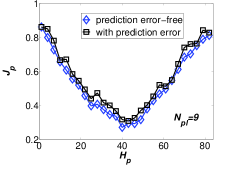
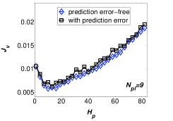
From the practical point of view, external perturbations (noise) and internal modeling mismatch are always present in any realistic systems, which inevitably induces some prediction error for the pseudo-leaders. To examine the influence of such prediction errors, we now introduce the perturbation into Eqs. (1) and (2) by adding an external two-dimensional white noise term $\xi\in[-\frac{1}{2}\eta,\frac{1}{2}\eta]\times[-\frac{1}{2}\eta,\frac{1}{2}\eta]$ to the vector $d_{pL}$, i.e., $\hat{d}_{pL}={d}_{pL}+\xi$ and $G(\hat{d}_{pL})=-\hat{d}_{pL}\left(a-b\cdot\mbox{exp}(-\|\hat{d}_{pL}\|_{2}^{2}/c)\right)$. The leader’s position is no longer perfectly known to the pseudo-leaders. From Fig. 7, one can observe that moderate external noises do not change the global behavior of the flock. The tendency of the curves $J_{p}$ and $J_{v}$ are almost the same as the noise-free case. Furthermore, to understand the capacity and robustness of our purposed predictive mechanism more deeply, we have also investigated the influences of stronger prediction errors $\xi$ with other kinds of leader trajectories including parabolic and sinusoidal curves in Appendix C. We found that the tolerance range of prediction error is large enough. In this way, the generality of the conclusions on the role of the predictive mechanism is thus further verified.

IV Predictive mechanisms in the Vicsek model

The role of predictive mechanisms highlighted in Section III is not merely confined to A/R flocks but quite general. To verify this, we now incorporate this predictive mechanism into another flocking model, i.e., the Vicsek model vi95 , and compare the synchronization performance of the predictive small-world Vicsek model with the one of the standard Vicsek model.

(a)

(b)

Figure 8: (Color online) (a) Snapshot of the predictive Vicsek flock at the $12^{th}$ running step. The red particle denotes the leader; the green particles represent the pseudo-leaders and the blue particles denote followers. The centered black circle outlines the trajectory of the leader. In this case, the prediction horizon is $H_{p}=4$. (b) Velocity synchronization index $J_{v}$ as a function of the parameters $H_{p}$ and $N_{pl}$. The parameters of this simulation are $L=15$, $\eta=0.1$, $v=0.15$, $N=300$, $r=1$, and $R=L/6$. The simulation result is averaged over $1000$ independent runs.

In this model, the velocities $v_{i}$ of the $N$ agents composing the group are determined simultaneously at each discrete-time instant, and the position of the $i$th agent is updated according to

$$x_{i}(k+1)=x_{i}(k)+v_{i}(k),$$

where $v_{i}(k)$ denotes the velocity vector of agent $i$ at time $k$. For each agent the velocity vector, $v_{i}(k)$, is characterized by a constant magnitude $v$ and by a direction $\theta_{i}(k)$ whose dynamics is given by

$$\theta_{i}(k+1)=\left<\theta_{i}\left(k\right)\right>_{r}+\Delta\theta_{i},$$

where $\left<\theta_{i}\left(k\right)\right>_{r}$ denotes the average direction of all the agents’ velocity vectors within a circle of radius $r$ centered on agent $i$, i.e.,

$$\left<\theta_{i}\left(k\right)\right>_{r}=\left\{\begin{array}[]{l}\mbox{arctan}\left[\left<\sin\left(\theta_{i}\left(k\right)\right)\right>_{r}/\left<\mbox{cos}\left(\theta_{i}\left(k\right)\right)\right>_{r}\right]\\ \quad\quad\mbox{if}~{}\left<\mbox{cos}\left(\theta_{i}\left(k\right)\right)\right>_{r}\geq 0;\\ \mbox{arctan}\left[\left<\sin\left(\theta_{i}\left(k\right)\right)\right>_{r}/\left<\mbox{cos}\left(\theta_{i}\left(k\right)\right)\right>_{r}\right]+\pi\\ \quad\quad\mbox{otherwise},\end{array}\right.$$

where $\left<\sin\left(\theta_{i}\left(k\right)\right)\right>_{r}$ and $\left<\mbox{cos}\left(\theta_{i}\left(k\right)\right)\right>_{r}$ denote the average sine and cosine values, and $\Delta\theta_{i}$ represents a random noise obeying a uniform distribution in the interval $[-\eta/2,\eta/2]$.

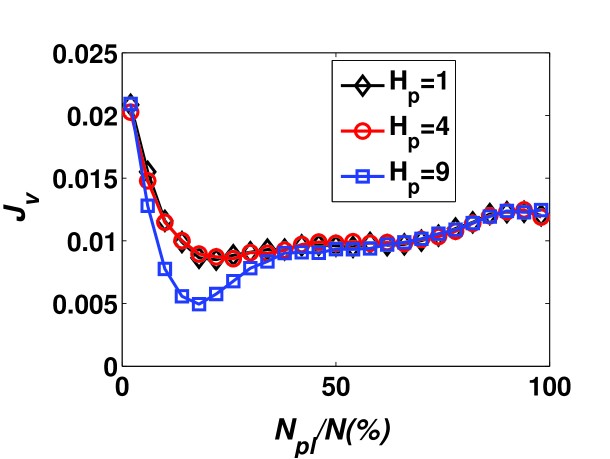
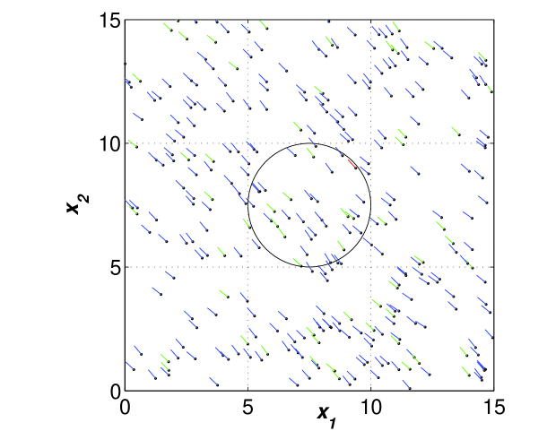
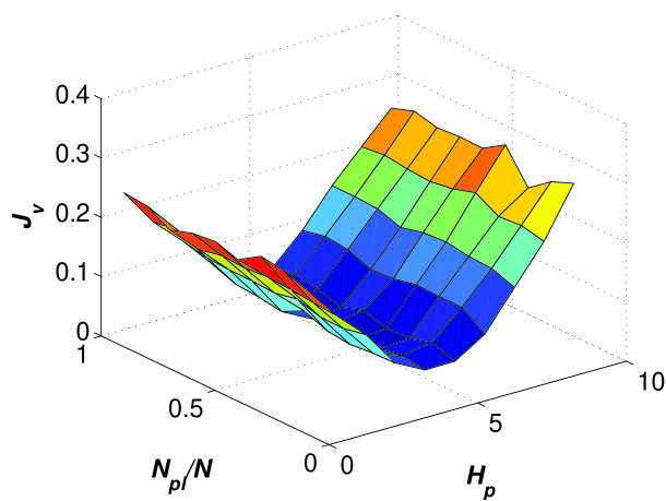
As shown in Fig. 8a the particles are distributed in a square of dimension $[0,L]\times[0,L]$. The trajectory of the leader, which is not affected by others, is a circle centered at $(L/2,L/2)$ with radius $R=L/6$ so that the direction of the leader changes constantly. The small-world predictive connection framework shown in Fig. 2 is used together with the Vicsek model. Hence, the $N_{pl}$ pseudo-leaders are always influenced by the leader’s velocity $H_{p}$ steps ahead together with its neighbors’ current velocities. It is shown in Fig. 8b that drastic improvement of the velocity synchronization performance can be achieved with moderate prediction horizons. Similar to the results of the A/R model shown in Section III, one can also conclude that suitable insight into the future and moderate number of pseudo-leaders is preferable.

V Conclusion and discussion

Inspired by the predictive mechanisms that universally exist in abundant natural bio-groups, we incorporate a certain predictive protocol into flocks with small-world structure. The predictive mechanism embedded in the pseudo-leaders lets many neighboring-connected followers know the current or even future dynamics of the leader in time, thus each individual can make a decision based on timely information of the leader instead of the delayed information as in some traditional models. In this way, the followers become more cohesive to the leader and the flock formation becomes more stable. Note that, in our model, the leader’s motion governs the trajectory of the whole swarm. However, it is a general feature of real migration flocks. Actually, in co05 , a changeable target known by a few leaders is used to guide the whole flock, in which only the target’s motion drives swarming behavior. Analogously, in this paper, a single leader is used to determine the general trajectory of the whole swarm. Therefore, the current leader-driven swarm is not unrealistic.

Simulation results led to the following conclusions: (i) Increasing the number of pseudo-leaders can always improve the cohesive flocking performance. Furthermore, it can improve the formation flocking performance when the pseudo-leader number has not exceeded a threshold, otherwise, the performance will be degraded. (ii) There exists a certain value of $H_{p}$ that optimizes the cohesive and the formation flocking performances, in other words, moderately increasing $H_{p}$ will improve the flocking performance, whereas predicting too many steps ahead will impair the flocking. (iii) Predictive capability and long-range links can compensate for the insufficiency of each other. It is worthwhile to emphasize the observed over-prediction phenomenon, which is of significance in practice.

Furthermore, to verify the generality of these conclusions, we have also applied the predictive mechanism to another popular flock model, the directed graph model with linear dynamics zh07 ; zh08 . The corresponding results also strongly suggest that predictive protocols are beneficial to flocking dynamics when taking into consideration both the flocking performance and the communication cost. More importantly, with this mechanism, only a very small proportion of the followers are required to act as the pseudo-leaders to achieve a better flocking performance, as measured by $J_{p}$ and $J_{v}$. From the industrial application point of view, the value of this work is two-fold: (i) The flocking performance is significantly improved by injection of a suitable predictive mechanism into the pseudo-leaders; (ii) Moderately increasing the predictive capability can help remarkably decrease the required number of pseudo-leaders. The latter feature is fairly useful for networks with insufficient long-range communication links, which are routinely costly.

This work provides a starting point aimed at achieving better flocking performance by using a predictive mechanism, and we hope that it will open new avenues in this fascinating direction.

Appendix A: Supplemental illustration of Fig. 5a

(a)

(b)

Figure 9: Supplemental illustration of Fig. 5a. In this scenario, pseudo-leader A moves nearly in the same direction of the leader, and degrading pseudo-leader C (see sub-figure (a)) into a follower (see sub-figure (b)) helps improve the velocity synchronization performance $J_{v}$.

We take a 4-agent flock for instance. As shown in Fig. 9a, all the individuals except the leader are pseudo-leaders. However, due to the repulsion between each couple of pseudo-leaders and the powerful attraction from the leader, the pseudo-leaders will keep certain distances between each other and form a section-like shape. Since all the pseudo-leaders always point to the leader’s predictive position $H_{p}$ steps ahead, the moving directions of all the individuals are obviously far from synchronized. By contrast, when one pseudo-leader C has been degraded into a follower as shown in Fig. 9b, and take into consideration that the followers are always lagging behind the pseudo-leaders, the direction of follower C is aligned to approach the heading of the leader more or less. In this way, the velocity synchronization performance $J_{v}$ is improved. Thus, too many pseudo-leaders are not preferred. For more general cases with prediction errors, more long-range connections will introduce larger deviation, which partially neutralize the positive effect of pseudo-leaders on $J_{v}$, thus moderate pseudo-leaders are also desirable.

Appendix B: Effects of the predictive mechanism with different leader’s trajectories

(a)	(b)
(c)	(d)

Figure 10: (Color online) The roles of the pseudo-leaders’ number $N_{pl}$ (figures (a) and (c)) and prediction horizon $H_{p}$ (figures (b) and (d)) on a flock with a total of $N=50$ agents. The trajectory of the leader is set along the sinusoidal curve defined by $x_{2}=\sin(2x_{1})+1$, and the velocity of the leader is $v_{L_{x_{1}}}(t)=0.02,~{}v_{L_{x_{2}}}(t)=\sin(0.04(t+1))-\sin(0.04t)$. The other parameters and initial conditions are the same as those in Fig. 5.

(a)	(b)
(c)	(d)

Figure 11: (Color online) The roles of the pseudo-leaders’ number $N_{pl}$ (figures (a) and (c)) and prediction horizon $H_{p}$ (figures (b) and (d)) on a flock with a total of $N=50$ agents. The trajectory of the leader is set along the parabolic curve defined by $x_{2}=x_{1}^{2}$, and the velocity of the leader is $v_{L_{x_{1}}}(t)=0.02,~{}v_{L_{x_{2}}}(t)=(0.02(t+1))^{2}-(0.02t)^{2}$. The other parameters and initial conditions are the same as those in Fig. 5

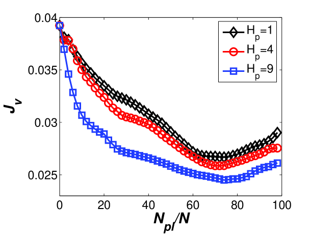
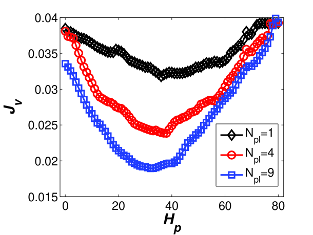
The conclusions drawn in this paper are not sensitive to the trajectory of the leader. In order to validate the generality of the conclusions on the role of predictive mechanisms, we have used another two different trajectories, i.e., sinusoidal ($x_{2}=\sin(2x_{1})+1$) and parabolic ($x_{2}=x_{1}^{2}$) curves. As shown in Fig. 9 and Fig. 10, no matter what the leader’s trajectory is, the influences of $H_{p}$ and $N_{pl}$ on the principal tendencies of both $J_{p}$ and $J_{v}$ remain the same. Those simulations suggest that our main conclusion, i.e., predictive capability and long-range links can compensate for the insufficiency of each other, is also valid in those two cases.

Appendix C: Effects of prediction errors

(a)	(b)
(c)	(d)
(e)	(f)

Figure 12: (Color online) The effects of prediction error $\xi$. Here, the trajectory of the leader is set along the curve defined by $x_{2}=\sqrt{x_{1}}$ (sub-figures (a) and (b)), $x_{2}=\sin(2x_{1})+1$ (sub-figures (c) and (d)) and $x_{2}=x_{1}^{2}$ (sub-figures (e) and (f)), respectively. The flock size is $N=50$, and the number of pseudo-leaders is $N_{pl}=9$. The other parameters and the initial conditions are the same as those in Fig. 5. Each point is averaged over 1000 independent runs. It can be found that moderate prediction error $\xi$ does not change the global behavior of the flock. If $\xi$, however, reaches a very large value, like $\eta=0.5$, the benefits of prediction capability on the synchronization $J_{v}$ will almost vanish. Note that, the curve of $J_{v}$ is more sensitive than that of $J_{p}$, making the feasible prediction error range of $J_{v}$ smaller than the counterpart of $J_{p}$.

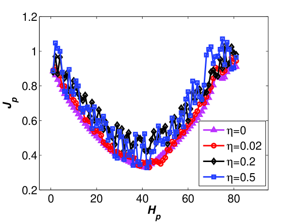
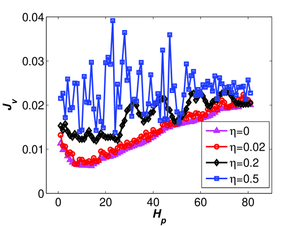
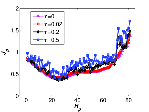
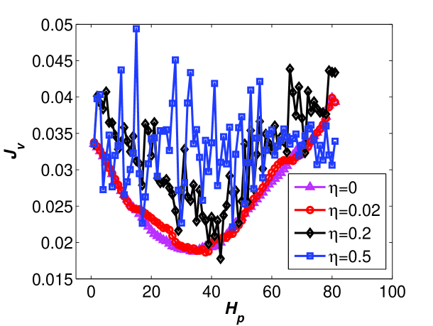
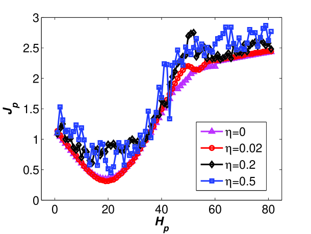
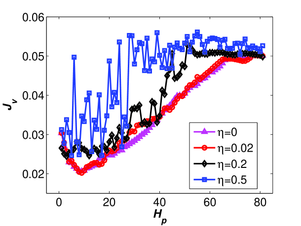
In realistic system models, mismatch and external perturbations which cause prediction errors are always present. For completeness, we hereby examine the effects of the prediction errors on synchronization behavior of the flock. As shown in Fig. 12, we present curves of $J_{v}$ and $J_{p}$ with increasing noise magnitude $\eta=0,0.02,0.2,0.5$ for the cases of three different leader trajectories (square root, parabolic and sinusoidal curves), respectively. It is observed that moderate prediction error $\xi$ ($\xi\leq 0.2$, for example) can hardly change the synchronization tendency of the flock, which guarantees the feasibility and superiority of the current predictive mechanism. On the contrary, too large $\xi$ ($\xi\geq 0.5$, for example) will inevitably impair the advantages of this predictive mechanism. This observation is reasonable, since every method has its own limits and one can not expect a poor prediction capability to yield a superb guidance for the flock. Fortunately, the tolerance range of prediction error is satisfactorily large, which further verifies the generality of our proposed predictive mechanism. Note that the curve of $J_{p}$ is more robust than the curve of $J_{v}$, which roots in that the relative velocities can be more easily deviated by prediction error than the relative positions.

References

- (1) Corresponding author, mzqchen@gmail.com
- (2) M. Aldana, V. Dossetti, C. Huepe, V. M. Kenkre, and H. Larralde, Phys. Rev. Lett. 98, 095702 (2007).
- (3) G. Grégoire and H. Chaté, Phys. Rev. Lett. 92, 025702 (2004).
- (4) T. Vicsek, A. Czirók, E. Ben-Jacob, I. Cohen and O. Shochet, Phys. Rev. Lett. 75, 1226 (1995).
- (5) M. R. D’Orsogna, Y. L. Chuang, A. L. Bertozzi and L. S. Chayes, Phys. Rev. Lett. 96, 104302 (2006).
- (6) H. Chaté, F. Ginelli and R. Montagne, Phys. Rev. Lett. 96, 180602 (2006).
- (7) J. P. Hernandez-Ortiz, C. G. Stoltz and M. D. Graham, Phys. Rev. Lett. 95, 204501 (2005).
- (8) W. Li, H.-T. Zhang, M. Z. Q. Chen and T. Zhou, Phys. Rev. E 77, 021920 (2008).
- (9) R. Olfati-Saber and R. Murray, IEEE. Trans. Autom. Contr. 49, 1520 (2004).
- (10) I. F. Akyildiz, W. Su, Y. Sankarasubramaniam and E. Cayirci, Computers Network 38, 393 (2002).
- (11) T. Arai, E. Pagello and L. E. Parker, IEEE Trans. Robotics and Automation 18, 1292 (2002).
- (12) D. Helbing, I. Farkas and T. Vicsek, Nature (London) 407, 487 (2000).
- (13) P. Ogren, E. Fiorelli and N. E. Leonard, IEEE Trans. Autom. Contr. 49, 1292 (2004).
- (14) D. J. Watts and S. H. Strogatz, Nature (London) 393, 440 (1998).
- (15) X. F. Wang, G. Chen, IEEE Trans. Circuits Syst. I 49, 54 (2002).
- (16) T. Zhou, M. Zhao, and B. H. Wang, Phys. Rev. E 73, 037101 (2006).
- (17) M. Aldana and C. Huepe, J. Stat. Phys. 112, 135 (2003).
- (18) C. W. Reynolds, ACM SIGGRAPH Computer Graphics 21, 25 (1987).
- (19) V. Gazi and K. M. Passino, IEEE Trans. Autom. Contr. 48, 692 (2003).
- (20) C. M. Breder, Ecology 35, 361 (1954).
- (21) K. Warburton and J. Lazarus, J. Theoret. Biolo. 150, 473 (1991).
- (22) B. I. Lev, Phys. Rev. E 58, 2681 (1998).
- (23) E. D. Belotskii and B. I. Lev, Phys. Lett. A 147, 13 (1990).
- (24) J. D. Weeks, K. Katsov and K. Vollmayr, Phys. Rev. Lett. 81, 4400 (1998).
- (25) A. J. Archer and N. B. Wilding, Phys. Rev. E 76, 031501 (2007).
- (26) P. Schlottmann, Phys. Rev. Lett. 68, 1916 (1992).
- (27) A. Melzer, V. A. Schweigert and A. Piel, Phys. Rev. Lett. 83, 3194 (1999).
- (28) F. Ohnesorge and G. Binnig, Science 260, 1451 (1993).
- (29) V. Gazi and K. M. Passino, IEEE Trans. Syst., Man, and Cybernetics 34, 539 (2004).
- (30) H. Shi, L. Wang and T. Chu, Physica D 213, 51 (2006).
- (31) C. Zimmer, “From ants to people, an instinct to swarm,” The New York Times, November 13, 2007.
- (32) Y. L. Chuang, M. R. D. Orsogna, D. Marthaler, A. L. Bertozzi, and L. S. Chayes, Physica D 232, 33 (2007).
- (33) X. Liu, J. Wang and L. Huang, Physica A 386, 543 (2007).
- (34) X. Liu, J. Wang and L. Huang, Physica A 383, 733 (2007).
- (35) L. Moreau, IEEE Trans. Autom. Control. 50, 169 (2005).
- (36) A. Jadbabaie, J. Lin and A. S. Morse, IEEE Trans. Autom. Contr. 48, 988 (2003).
- (37) E. F. Woods, Nature (London) 184, 842 (1959).
- (38) P. R. Montague, P. Dayan, C. Person and T. J. Sejnowski, Nature (London) 377, 725 (2002).
- (39) J. A. Gottfried, J. O. Doherty and R. J. Dolan, Science 301, 1104 (2003).
- (40) C. Summerfield, T. Egner, M. Greene, E. Koechlin, J. Mangles and J. Hirsch, Science 314, 1311 (2006).
- (41) D. Melcher, Nature Neuroscience 10, 903 (2007).
- (42) I. D. Couzin, J. Krause, N. R. Franks and S. A. Levin, Nature (London) 433, 513 (2005).
- (43) In this paper, a trajectory is considered to be “regular” if it preserves a continuous, differentiable curves, like parabolic, sinusoidal and circular waves, along with the increasing time variable . Moreover, it should not contain any large fluctuation or some chaos-like movement so that its future tendency can be predicted by smoothing the historical sequence. For instance, when catching a frisbee, a dog will make prediction on its historical parabolic trajectory, and head for the predicted point of fall. In this case, the trajectory of the frisbee is “regular”, and this kind of examples often happen in the real world.
- (44) J. Krause and G. D. Ruxton, Living in Groups, Oxford Univ. Press, Oxford (2002).
- (45) H. T. Zhang, G. B. Stan, M. Z. Q. Chen, J. M. Maciejowski and T. Zhou, arXiv: 0709.0172 (2007).
- (46) H. T. Zhang, M. Z. Q. Chen, T. Zhou and G.-B. Stan, Europhys. Lett. 83, 2008 (to appear).