Abstract

We find exact solutions in five dimensional inhomogeneous matter dominated model with a varying cosmological constant. Adjusting arbitrary constants of integration one can also achieve acceleration in our model. Aside from an initial singularity our spacetime is regular everywhere including the centre of the inhomogeneous distribution. We also study the analogous homogeneous universe in (4+d) dimensions. Here an initially decelerating model is found to give late acceleration in conformity with the current observational demands. We also find that both anisotropy and number of dimensions have a role to play in determining the time of flip, in fact the flip is delayed in multidimensional models. Some astrophysical parameters like the age, luminosity distance etc are also calculated and the influence of extra dimensions is briefly discussed. Interestingly our model yields a larger age of the universe compared to many other quintessential models.

KEYWORDS : cosmology; higher dimensions; varying $\Lambda$

PACS : 04.20, 04.50 +h

1. Introduction

Recent observational evidences suggest that the present day universe has the critical energy density containing presumably $70\%$ dark energy and about $30\%$ dark matter, where the term dark indicates a sort of invisibility. While the sceptics will always question the wisdom to explain data based on something we can not see the avalanche of data emanating from type Ia supernovae measurements [1], CMB anisotropies [2], galactic rotation curves and surveys of galaxies, clusters and superclusters make the presence of dark matter and dark energy increasingly convincing. This situation inevitably forces us to pose the question : why are dark matter and dark energy so dark ?

As a natural corollary to the question one is reminded of another ‘dark’ stuff in physics, extra dimensions. Like dark matter and dark energy to explain the current quintessential behaviour the existence of extra dimensions is absolutely necessary in any attempt to unify gravity with other forces of nature beyond the standard model of particle physics and also to explain the vexed hierarchial problem of quantum mechanics in varied brane inspired models [3]. The recent spurt in activities in extra dimensions also stems from the Space-Time-Matter (STM) theory [4] proposed recently by Wesson and his collaborators [5]. As our space time is manifestly four dimensional in nature the extra dimensions should be ‘hidden’ ( or ‘dark’ ).

In the back drop of the above discussions it is more than apparent that this common feature of ‘invisible existence’ of dark matter, dark energy and extra dimension points to the conjecture that there must be some deep underlying relationship and inter play among them [6].

Motivated by this consideration we have in the past worked out problems [5] where starting from a perfect fluid in higher dimensions obeying reasonable energy conditions accelerating model is made possible as a consequence of the existence of higher dimensions. Interestingly we do not have to invoke any adhoc quintessential type of fluid by hand to achieve the acceleration.

The motivation for the present work is somewhat different. In an earlier communication [7] we have analysed an inhomogeneous 5D spacetime with a constant $\Lambda$, and showed that unlike the finding of Tosa [8] the spacetime did show the desirable feature of dimensional reduction as the usual 3D space expands. Although in the light of observational evidences that our universe is currently accelerating, the idea of $\Lambda$ is now an integral ingredient in cosmological models its introduction, nevertheless, invites serious conceptual problems. The upper limit of $\Lambda$ from observations is about 120 orders of magnitude below the value for the vacuum energy density predicted from quantum field theory.

To circumvent this difficulty and a host others an essentially phenomenological approach is generally taken where it is argued that due to the coupling of the dynamical degrees of freedom with matter fields of the universe, $\Lambda$ relaxes to its current small value through the expansion of the Universe and creation of photons [9]. From this point of view $\Lambda$ is small because the Universe is old.

Another salient feature of our model is its inhomogeneity. While the higher dimensional generalisation of the FRW models has been adequately addressed in the literature scant attention has been paid so far to address the inhomogeneous situations and the issues coming out from it. Moreover the work of Mustapha etal [10] and others indicate that there is no unquestionable observational evidences for spatial homogeneity. So investigations in inhomogeneous models is always a welcome step.

Although the cosmological concordance $\Lambda CDM~{}~{}models$ fit most of the observations well, as mentioned earlier, it is beset with theoretical difficulties. In fact whenever there is any ambiguity interpreting any observational results as in 1990s regarding the age of the universe [11] the inhomogeneous models are seriously considered. Similarly in the backdrop of the current accelerating phase of the universe the role of inhomogeneities [12] like that of extra dimensions as a possible ingredient of the cause of the apparent acceleration is being increasingly debated [13]. In fact averaging out the spatial degrees of freedom ( i.e. inhomogeneities) leads to averaged, effective Einstein equations (somewhat similar to what we find in higher dimensional models also), which contain some additional terms relating to the inhomogeneous distributions generally termed back reaction in this context. It is argued that this so called back reaction can account for the current acceleration of the universe [14]. Our scope in the present work is very limited. While we have attempted to address the implications of extra dimensions in the context of current accelerating expansion in some detail the role inhomogeneities in our present model has been deferred to a future work in progress.

The paper is organised as follows: in section 2 we find an exact solution for a 5D inhomogeneous distribution with a variable $\Lambda$. Interestingly we here get acceleration, although at the cost of sacrificing dimensional reduction. In section 3 we focus on a homogeneous (d+4)-dimensional spacetime to show that accelerating model is possible in this case also. In section 4 some important astrophysical parameters are discussed for our model to investigate how inclusion of extra dimensions influences the situation. Section 5 compares the $\Lambda$ varying case with our earlier $\Lambda$- constant situation. Here an initially decelerating universe ends up as an accelerating one. Here we find two interesting results- both anisotropy and number of dimensions have marked effects in determining the instant of flip. The paper ends with a brief discussion in section 6.

2. The Field Equations and its integrals

We consider a metric of (3 + d + 1)-dimensional spacetime where both the ordinary 3-space and the extra ( or hidden) space are inhomogeneous, isotropic and flat :

$$ds^{2} = dt^{2}-a^{2}\left[dr^{2}+r^{2}\left(d\theta^{2}+r^{2}sin^{2}\theta d\phi^{2}\right)\right]-b^{2}dy^{2}$$ (1)

$dy^{2}=\sum^{d}_{i=1}dy^{2}_{i}$ and we assume a single scale factor for the internal dimensions, here a(r,t) and b(r,t) are scale factors. Assuming that the matter content in this higher dimensional space is taken to be a perfect fluid and is augmented by the inclusion of a time varying cosmological constant we can write down the Einstein’s equations, which govern the evolution of the ordinary 3-space as well as the extra space as

$$G_{01}=2\frac{\dot{a^{\prime}}}{a}-2\frac{\dot{a}a^{\prime}}{a^{2}}+d\left(\frac{\dot{b^{\prime}}}{b}-\frac{\dot{a}b^{\prime}}{ab}\right)=0\\$$ (2)

$$G^{1}_{1}=2\frac{\ddot{a}}{a}+\frac{\dot{a^{2}}}{a^{2}}+2d\frac{\dot{a}\dot{b}}{ab}+\frac{d(d-1)}{2}\frac{\dot{b^{2}}}{b^{2}}+d\frac{\ddot{b}}{b}~{}~{}~{}~{}~{}~{}~{}~{}~{}~{}~{}~{}~{}~{}~{}~{}~{}~{}~{}~{}~{}~{}~{}~{}~{}~{}~{}~{}~{}~{}~{}~{}~{}~{}~{}~{}~{}~{}~{}~{}~{}~{}~{}~{}~{}~{}~{}~{}~{}~{}~{}~{}~{}~{}~{}~{}~{}~{}~{}~{}~{}~{}~{}~{}~{}~{}~{}~{}~{}$$

$$~{}~{}~{}~{}~{}-\frac{1}{a^{2}}\left[2\frac{a^{\prime}}{ar}+2d\frac{b^{\prime}}{br}+2d\frac{a^{\prime}b^{\prime}}{ab}+\frac{a^{\prime 2}}{a^{2}}+\frac{d(d-1)}{2}\frac{b^{\prime 2}}{b^{2}}\right]=-p+\Lambda~{}~{}~{}~{}~{}~{}~{}~{}~{}~{}~{}~{}~{}~{}~{}~{}~{}~{}~{}~{}~{}~{}~{}~{}$$ (3)

$$G^{2}_{2}=G^{3}_{3}=2\frac{\ddot{a}}{a}+\frac{\dot{a^{2}}}{a^{2}}+2d\frac{\dot{a}\dot{b}}{ab}+\frac{d(d-1)}{2}\frac{\dot{b^{2}}}{b^{2}}+d\frac{\ddot{b}}{b}~{}~{}~{}~{}~{}~{}~{}~{}~{}~{}~{}~{}~{}~{}~{}~{}~{}~{}~{}~{}~{}~{}~{}~{}~{}~{}~{}~{}~{}~{}~{}~{}~{}~{}~{}~{}~{}~{}~{}~{}~{}~{}~{}~{}~{}~{}~{}~{}~{}~{}~{}~{}~{}~{}~{}~{}~{}~{}~{}~{}~{}$$

$$-\frac{1}{a^{2}}\left[\frac{a^{\prime\prime}}{a}-\frac{a^{\prime 2}}{a^{2}}+\frac{a^{\prime}}{ar}+d\frac{b^{\prime}}{br}+\frac{d(d-1)}{2}\frac{b^{\prime 2}}{b^{2}}+d\frac{b^{\prime\prime}}{b}\right]=-p+\Lambda~{}~{}~{}~{}~{}~{}~{}~{}~{}~{}~{}~{}~{}~{}~{}~{}~{}~{}~{}~{}~{}~{}~{}~{}~{}~{}$$ (4)

$$G^{4}_{4}=3\frac{\ddot{a}}{a}+3\frac{\dot{a^{2}}}{a^{2}}+3(d-1)\frac{\dot{a}\dot{b}}{ab}+\frac{(d-1)(d-2)}{2}\frac{\dot{b^{2}}}{b^{2}}+(d-1)\frac{\ddot{b}}{b}~{}~{}~{}~{}~{}~{}~{}~{}~{}~{}~{}~{}~{}~{}~{}~{}~{}~{}~{}~{}~{}~{}~{}~{}~{}~{}~{}~{}~{}~{}~{}~{}~{}~{}~{}~{}~{}~{}~{}~{}~{}~{}~{}~{}~{}~{}~{}$$

$$-\frac{1}{a^{2}}\left[2\frac{a^{\prime\prime}}{a}-4\frac{a^{\prime}}{ar}\frac{a^{\prime 2}}{a^{2}}+(d-1)\frac{a^{\prime}b^{\prime}}{ab}+2(d-1)\frac{b^{\prime}}{br}+(d-1)(d-2)\frac{b^{\prime 2}}{b^{2}}+(d-1)\frac{b^{\prime\prime}}{b}\right]~{}~{}~{}~{}~{}~{}~{}~{}~{}~{}~{}~{}~{}~{}~{}$$

$$=-p_{d}+\Lambda~{}~{}~{}~{}~{}~{}~{}~{}~{}~{}~{}~{}~{}~{}~{}~{}~{}~{}~{}~{}~{}~{}~{}~{}~{}~{}~{}~{}~{}$$ (5)

$$G^{0}_{0}=3\frac{\dot{a^{2}}}{a^{2}}+\frac{d(d-1)}{2}\frac{\dot{b^{2}}}{b^{2}}+3d\frac{\dot{a}\dot{b}}{ab}~{}~{}~{}~{}~{}~{}~{}~{}~{}~{}~{}~{}~{}~{}~{}~{}~{}~{}~{}~{}~{}~{}~{}~{}~{}~{}~{}~{}~{}~{}~{}~{}~{}~{}~{}~{}~{}~{}~{}~{}~{}~{}~{}~{}~{}~{}~{}~{}~{}~{}~{}~{}~{}~{}~{}$$

$$-\frac{1}{a^{2}}\left[2\frac{a^{\prime\prime}}{a}-\frac{a^{\prime 2}}{a^{2}}+4\frac{a^{\prime}}{ar}+d\frac{a^{\prime}b^{\prime}}{ab}+2d\frac{b^{\prime}}{br}+\frac{d(d-1)}{2}\frac{b^{\prime 2}}{b^{2}}+d\frac{b^{\prime\prime}}{b}\right]=\rho+\Lambda$$ (6)

where the (3+d+1)-dimensional stress-tensor, $T_{ij}$, in comoving co-ordinate should be of the form

$$T^{0}_{0}=\rho+\Lambda,T^{1}_{1}=T^{2}_{2}=T^{3}_{3}=-p+\Lambda,T^{d}_{d}=-p_{d}+\Lambda$$ (7)

We have here assumed that $8\pi\bar{G}=1$ where $\bar{G}$ is the gravitational constant in the higher dimensional space and a dot and and a prime overhead denote differentiation w.r.t. time and radial co-ordinate.

To make the field equations tractable we assume, at this stage, that the scale factors $a\equiv a(t)$ and $b\equiv b(r,t)$ and d = 1, i.e., we take a 5D spacetime where the $y$ = constant hypersurface is homogeneous FRW-like. In what follows we shall see that the fact that inhomogeneity is being introduced through the extra space has far reaching implications in the cosmological evolution of our models. For simplicity as also the fact that the present universe is matter dominated, we consider here the dust case only ($p=p_{d}=0$).

Now the equation (2) yields

$$b=a\beta(r)+\alpha(t)$$ (8)

where $\beta(r)$ and $\alpha(t)$ are integration functions of r and t respectively. Using equations (3), (4) and (8) we get

$$b=-cr^{2}a+\alpha(t)$$ (9)

where c is a pure constant. However we subsequently see that c is not exactly arbitrary, being a measure of the curvature of the 4D space. Moreover $c=0$ implies at once a flat and homogeneous spacetime. In line with the existing literature one assumes the dynamical behaviour of $\Lambda$ as $\Lambda\sim(\frac{\dot{a}}{a})^{2},\Lambda\sim\frac{\ddot{a}}{a}$ or $\Lambda\sim\rho$. Although not strictly independent the first one was proposed from dimensional consideration by Lima and Waga [15] and subsequently adopted by several workers [16], [17] whereas the second type by Overduin and Cooperstock [18] while Vishwakarma [9] favoured the third alternative.

In our work we take $\Lambda=kH^{2}$,$(H\equiv\frac{\dot{a}}{a})$ which through equation (5) yields $a=t^{\frac{3}{(6-k)}}$ and $\Lambda=\frac{9k}{(6-k)^{2}}t^{-2}$ . Now using equation (3) we get,

$$\ddot{\alpha}+\frac{6}{(6-k)}\dot{\alpha}t^{-1}-3\frac{(3+k)}{(6-k)^{2}}t^{-2}\alpha+4ct^{-\frac{3}{(6-k)}}=0$$ (10)

which through a long but somewhat straight forward calculation yields

$$\alpha=a_{1}t^{\frac{3}{(6-k)}}+a_{2}t^{-\frac{(3+k)}{(6-k)}}-\frac{2c(6-k)^{2}}{(12-k)(3-k)}t^{\frac{(9-2k)}{(6-k)}}\\$$ (11)

$a_{1}$, $a_{2}$ are arbitrary constants. So clubbing everything together we finally get

$$a = t^{\frac{3}{(6-k)}}$$ (12)

$$b = (a_{1}-cr^{2})t^{\frac{3}{(6-k)}}+a_{2}t^{-\frac{(3+k)}{(6-k)}}-\frac{2c(6-k)^{2}}{(12-k)(3-k)}t^{\frac{(9-2k)}{(6-k)}}$$ (13)

$$\rho = \frac{\frac{9}{(6-k)}(a_{1}-cr^{2})t^{2\frac{(k-3)}{(6-k)}}+\frac{9(3-2k)}{(6-k)^{2}}a_{2}t^{\frac{12-k}{k-6}}-\frac{6ck(6-k)}{(12-k)(3-k)}}{(a_{1}-cr^{2})t^{\frac{6}{(6-k)}}+a_{2}t^{\frac{-k}{6-k}}-2c\frac{(6-k)^{2}}{((12-k)(3-k)}t^{2}}$$ (14)

$$\Lambda = \frac{9k}{(6-k)^{2}}t^{-2}$$ (15)

One can now calculate the 4-space curvature $\left(R^{*(4)}\right)$ of the t-constant slice for the line element (1)$(d=1)$ through the expression,  $R^{i}_{i}=R^{*(4)}+\dot{\theta}+\dot{\theta}^{2}-2\omega^{2}+u^{i}_{;i}$  [19], where $\theta$ is the expansion scalar and last two terms refer to vorticity and acceleration. After some algebra we get the expression

$$R^{*(4)}=\frac{12c}{(a_{1}-cr^{2})t^{\frac{6}{(6-k)}}+a_{2}t^{-\frac{k}{(6-k)}}-\frac{2ct^{2}(6-k)^{2}}{(12-k)(3-k)}}$$ (16)

So as commented earlier, the arbitrary constant $c$ comes out to be a measure of the curvature of the 4D space. $c$ is also a measure of inhomogeneity parameter because $c=0$ makes our spacetime homogeneous. Relevant to mention that unlike the analogous homogeneous case here the curvature also depends on spatial co-ordinate $r$. Moreover it blows off at the initial singularity $t=0$. Otherwise it is regular everywhere including the origin of the distribution.

To check if our space time contains any geometric singularity aside from the well known $t=0$ big bang epoch we calculate the Kretschmann scalar for our 5D inhomogeneous line element as

$$R^{ijkl}R_{ijkl}=3\frac{\ddot{a}^{2}}{a^{2}}+\frac{\ddot{b}^{2}}{b^{2}}+3\frac{\dot{a}^{4}}{{a}^{4}}+2\left(\frac{\dot{a}}{a}\frac{\dot{b}}{b}-\frac{1}{a^{2}}\frac{b^{\prime}}{br}\right)^{2}$$ (17)

At $t\rightarrow 0$, the invariant diverges but it is regular at $r=0$ since $\frac{b^{\prime}}{r}$ is regular there. So unlike similar cases in many inhomogeneous distributions there is no spatial singularity in our cosmological model including the centre of distribution. Moreover it has not escaped our notice that while the 3D scale factor $a$ starts from $t=0$ the 5D scale $b$ is infinite there. To ensure that both the scales start simultaneously at the initial singularity we set the arbitrary constant $a_{2}$ to be zero henceforth.

The inhomogeneous metric we presented here is very general in nature in the sense that many well known solutions in this field are recoverable as special cases of our metric.

(i) When $k=0$ the $\Lambda$ term vanishes and we get back our earlier solution [20].

(ii)If $k=0$ , $c=a_{1}=0$, we get $a\sim t^{\frac{1}{2}}$, $b\sim t^{-\frac{1}{2}}$ and $\rho$ = 0 which is the well known vacuum solution of Chodos and Detweiler [21].

(iii) Further for $c=a_{2}=0$, we recover the isotropic solution of Gr$\o$n [22].

If we now calculate the 3D deceleration parameter,

$$q=-\frac{\ddot{a}/a}{\dot{a}^{2}/a^{2}}=\frac{(3-k)}{3}$$ (18)

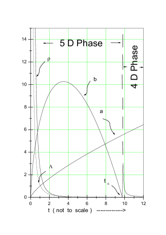
such that $k>3$ for accelerating model. From equation (12) it is evident that as we are discussing an expanding universe $k<6$. Moreover, the second metric co-efficient b is regular when $k<\frac{9}{2}$. Further, when $c>0$ and $0<k<3$ we get dimensional reduction but no acceleration. It also follows from equation (13) that for $(a_{1}-cr^{2})>0$, $c>0$ and $0<k<3$, the mass density also remains non-negative as is also evident from figure 1. Let us consider the situation for $c<0$. In this case $\rho$ is always positive. If we further subdivide the situation for (i) $0<k<3$ and (ii) $3<k<\frac{9}{2}$, we see for case (i) $\rho>0$, but no dimensional reduction is possible and no acceleration, for the case (ii) while $\rho$ is again positive, we interestingly get both dimensional reduction and acceleration. However small extra dimensions have of late been somewhat out of favour following the resurgence of interests in different brane inspired cosmological models where the extra dimensions need not be small to account for the vexed hierarchial problem of particle field theory.

It is conjectured that during the process of dimensional reduction the extra dimensions finally stabilize at a very small length and loose their dynamical character before the extra scale factor $b$ vanishes. Thereafter the cosmology enters the 4D phase without having any reference to the extra dimensions [29]. So the second singularity at $b=0$ is never reached and the invariants of equations (16-17) as also the mass density never have the chance to diverge there. For this model this transition has far reaching implications because the very existence of the extra space, so to speak, seems to induce inhomogeneity in this case. So not only do we enter a 4D era, it also envisages a smooth transition from a multidimensional, inhomogeneous phase to a 4D homogeneous one. Interestingly this transition takes place without forcing ourselves to choose very special initial conditions as is the practice in the four dimensional cosmology. This, in our opinion is a very important aspect of our model. So the primordial inhomogeneities die down in a natural way.

Figure 1: The time evolution of a, b, $\rho$ and $\Lambda$ are shown in this figure for $c>0$ and $0<k<3$ (say, $(a_{1}-cr^{2})=10,~{}k=2,~{}a_{2}=0$ and $c=1$ ). In this case dimensional reduction is possible but no acceleration. At compactification $t=t_{c}$, $\rho$ surges to infinity and cosmology enters 4D phase

3. Homogeneous and Isotropic Universe

As our universe is now manifestly homogeneous and isotropic we assume a = b and also the metric coefficients depend on time alone. These assumptions also facilitate to make comparison with the observational results as also to gauge the influence of extra dimensions on the recent observational findings.

With these two assumptions our general field equations (1) now reduce to

$$\frac{(d+2)(d+3)}{2}\frac{\dot{a}^{2}}{a^{2}} = \rho+\Lambda$$ (19)

$$(d+2)\frac{\ddot{a}}{a}+\frac{(d+1)(d+2)}{2}\frac{\dot{a}^{2}}{a^{2}} = \Lambda$$ (20)

As there are two independent equations with three unknowns we once again assume $\Lambda=kH^{2}$. With this assumption we finally get,

$$a = (Ct+D)^{\frac{2(d+2)}{(d+2)(d+3)-2k}}$$ (21)

$$\rho = \frac{2(d+2)^{2}}{(d+2)(d+3)-2k}t^{-2}$$ (22)

$$\Lambda = \frac{4k(d+2)^{2}}{\left[(d+2)(d+3)-2k\right]^{2}}t^{-2}$$ (23)

$$H = \frac{2(d+2)}{(d+2)(d+3)-2k}t^{-1}$$ (24)

we can set the constant $C=1$ and $D=0$ without loss of generality in equation (21). Further the positivity of $\rho$ gives the restriction $k<\frac{(d+2)(d+3)}{2}$

As a special case to our solution (21) we see that

(i) $k=0$ ( i.e. , $\Lambda=0$ ) implies $a=t^{\frac{2}{d+3}}$ which is the higher dimensional generalization of the well known Einstein- de Sitter solution.

(ii) further for the usual 4D case ($d=0$) $a\sim t^{\frac{2}{3}}$ which is the FRW matter dominated case.

(iii) on the other hand $d=0$, but $\Lambda\neq 0$ , $a\sim t^{\frac{2}{3-k}}$ [23]

Characteristics of the Model

From equation (19)

$$\frac{\rho}{\frac{(d+2)(d+3)}{2}H^{2}}+\frac{\Lambda}{\frac{(d+2)(d+3)}{2}H^{2}}=1$$ (25)

or $\Omega_{m}+\Omega_{\Lambda}=1$ ( in the absence of curvature term ) where $\Omega_{m}$ is the higher dimensional cosmic matter density parameter and $\Omega_{\Lambda}$ is the corresponding vacuum energy density parameter. From equations (21) - (25) it also follows that $\Omega_{m}=\frac{(d+2)(d+3)-2k}{(d+2)(d+3)}$ and $\Omega_{\Lambda}=\frac{2k}{(d+2)(d+3)}$ such that $\Omega_{m}+\Omega_{\Lambda}=1$. So our solutions are consistent. It also follows from the expression of $\Omega_{\Lambda}$ that the arbitrary constant k is also a measure of the cosmic vacuum density parameter. We further see that the deceleration parameter comes out to be

$$q=-\frac{\ddot{a}}{aH^{2}}=\frac{(d+1)(d+2)-2k}{2(d+2)}=\frac{(d+1)-(d+3)\Omega_{\Lambda}}{2}$$ (26)

For our cosmology to accelerate $k>\frac{(d+1)(d+2)}{2}$ such that we finally restrict $k$ as $\frac{(d+1)(d+2)}{2}<k<\frac{(d+2)(d+3)}{2}$. This inequality ensures that we get both positivity of $\rho$ and acceleration. To make our analysis consistent with the present day observational results we find that for $q=-0.5$, $k=\frac{(d+2)^{2}}{2}$. For the particular case of 5D universe ($d=1$), taking the most acceptable value of $H_{0}$ = 72 km/s/mpc we calculate the age of the universe to be equal to 25.5 Gyr, quite large. Almost same age was obtained by Viswakarma [24] in a different context. Another point to mention is that the above value of k implies (for $d=1$) $\Omega_{m0}=0.25$ and $\Omega_{\Lambda 0}=0.75$, which are fairly consistent with current observational results.

Another attractive feature of our model is that it gives a sufficiently large age of the Universe as mentioned earlier. It is evident from our equation (24) that the age of the universe for our model comes out to be $t_{0}=\frac{3}{(6-k)H_{0}}$ (for $d=1$). This is very remarkable in view of the fact that the age of the universe in the FRW model with a constant $\Lambda$ is uncomfortably close to the age of the globular clusters $t_{GC}=12.5\pm 1.2$ Gyr [25]. The quintessential models give even lower age. As there is considerable uncertainty in the exact value of $H_{0}$ we have calculated $\Omega_{\Lambda 0}$ and $t_{0}$ for different value of k, keeping $H_{0}$ a constant for a particular table as shown below.

Table 1: Age of the universe for different values of $H_{0}$ (for d = 1)

k	q	$\Omega_{\Lambda 0}$	$\Omega_{m0}$	t(Gyr)	t(Gyr)	t(Gyr)
				$H_{0}$ = 72 km/s/mpc	$H_{0}$ = 80 km/s/mpc	$H_{0}$ = 100 km/s/mpc
0.00	1.00	0.00	1.00	6.25	5.63	4.50
1.00	0.67	0.17	0.83	7.50	6.75	5.40
2.00	0.33	0.33	0.67	9.38	8.44	6.75
3.00	0.00	0.50	0.50	12.50	11.25	9.00
3.50	-0.17	6.75	8.44	11.25	13.50	16.88
4.00	-0.33	0.67	0.33	18.75	16.88	13.50
4.50	-0.50	0.75	0.25	25.00	22.50	18.00

Next we have plotted the age of the universe $t_{0}$ against $\Omega_{\Lambda 0}$ on the basis of our model. It is found that as $\Omega_{\Lambda 0}$ increases $t_{0}$ also increases. If the required mass density $\Omega_{m0}$ was smaller or $\Omega_{\Lambda 0}$ is larger one could get higher age in these model as is clear from figure 2.

Figure 2: As $\Omega_{\Lambda 0}$ increases ( or $\Omega_{m0}$ decreases ) $t_{0}$ increases

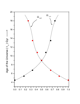
Again we see from the table 1 that the gradual increases of $H_{0}$ provide the more realistic age of the Universe, for $H_{0}$ = 100 km/s/mpc, the age of the universe $t_{0}$ = 18 Gyr whereas the most acceptable age of being 14 Gyr [23]. We also see from the table 1 that for k = 3, q = 0, i.e. , the flip occurs for this value of k. For $H_{0}$ = 100 km/s/mpc, the flip time $t_{f}$ = 9 Gyr, i.e., before it the universe decelerates. So our model $\Lambda\sim H^{2}$ is amenable to past deceleration and current acceleration.

4. Influence of Dimension

(i) Age of the Universe :

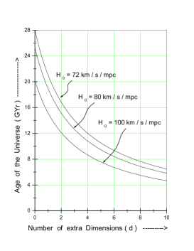
If we calculate $t_{0}=\frac{2}{(d+3)\Omega_{m0}H_{0}}$ (see equation (24)), taking the most acceptable values of $\Omega_{m0}$ = 0.33 and $H_{0}=72\pm 8~{}km/s/mpc$ and then plot $t_{0}\sim d$ curve the age of the universe is found to decrease with the number of dimensions of the universe. This is a very interesting result of our whole analysis ( see figure 3).

Figure 3: This figure shows that as the number of dimension increases age of the universe decreases

(ii) Cosmological constant :

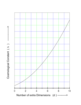
The relation between $\Lambda$ with the number of dimensions of the universe is written as

$$\Lambda=\frac{1}{2}H_{0}^{2}(1-\Omega_{m0})(d+2)(d+3)$$ (27)

If we plot $\Lambda\sim d$ one sees that $\Lambda$ increases as the number of extra dimensions (d ) increases (figure 4).

Figure 4: As the number of dimension increases $\Lambda$ also increases

(iii) Deceleration Parameter :

$$q=\frac{1}{2}\left[(\Omega_{m0}d-3(1-\Omega_{m0})\right]$$ (28)

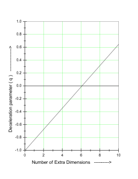
The above equation implies that as the number of dimensions increases $q$ increases. For constant $\Omega_{m0}$ it is shown that $q\propto d$. The figure 5 shows that (for $\Omega_{m0}$ = 0.33 ) as the number of dimensions increases, $q$ increases. Obviously the flip is delayed with the increase of number of dimensions for any particular value of $\Omega_{m0}$.

Figure 5: q increases with the number of dimensions

5. Some Astrophysical Parameters in our model :

In this section we shall very briefly discuss the proper distance D(z), luminosity distance ($D_{L}$) and look back time. As these quantities are extensively discussed for 4D space time in the standard text books [26] we shall omit detailed mathematical calculations and give only the final results generalised to ( 4 + d ) dimensions for our dust model.

(i) Proper Distance : Let a star located at $r=r_{0}$ emit radiation at $t=t_{1}$ and an observer at $r=0$ receive the same at $t=t_{0}$. The path being evidently a null geodesic ($\theta_{1},\theta_{2},\theta_{3}.....,\theta_{n}=constants$). The proper distance between the source and observer is given by

$$D(z)=a_{0}\int_{a}^{a_{0}}\frac{da}{a\dot{a}}=H_{0}^{-1}\left[\frac{2(d+2)}{(d+2)(d+1)-2k}\right]\left[1-(1+z)^{\frac{2k-(d+2)(d+1)}{2(d+2)}}\right]$$ (29)

for small z it reduces to,

$$H_{0}D(z)=z-\frac{(d+2)(d+3)-2k}{4(d+2)}z^{2}+.....=z-\frac{1}{2}(1+q)z^{2}+...$$ (30)

Again, for $z\rightarrow\infty$ but no acceleration i.e., $k<\frac{1}{2}(d+1)(d+2)$,
$D(z=\infty)=H_{0}^{-1}\frac{2(d+2)}{(d+1)(d+2)-2k}=\frac{H_{0}^{-1}}{q}=\frac{H_{0}^{-1}}{2\Omega_{m0}-1}$, for acceleration obviously $D(z)\rightarrow\infty$

(ii) Luminosity Distance $D_{L}$ : Luminosity distance is another very useful concept of relativistic astrophysics. If $D_{L}$ is the luminosity distance of the object, L being the total energy emitted by a Galaxy in unit time then

$$D_{L}=\left(\frac{L}{4\pi l}\right)^{\frac{1}{2}}$$ (31)

After some straight forward calculation we get for our model

$$H_{0}D_{L}=\frac{2(d+2)}{(d+1)(d+2)-2k}(1+z)\left[1-(1+z)^{\frac{2k-(d+1)(d+2)}{2(d+2)}}\right]$$ (32)

for small z,

$$H_{0}D_{L}=z+\frac{1}{2}(1-q)z^{2}=z+\frac{1}{4}\left[5-\Omega_{m0}(d+1)\right]z^{2}$$ (33)

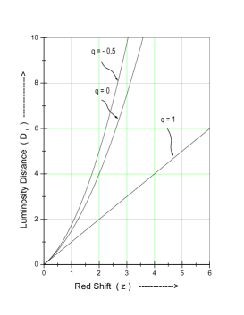
Figure 6: The Luminosity distance $D_{L}$ expressed as a function of the redshift $z$ for $q=1,0,-0.5$. The relationship is linear, as predicted by Hubble’s linear Law. For $q_{0}=-0.5$, $D_{L}$ increases faster. All curves merge for small z

We have plotted $D_{L}(q_{0},z)$ as a function of $z$ for various parametric values of $q_{0}$ in the figure 6. Note that all curves start off with the linear Hubble law $z=H_{0}D_{1}$ for small value of $z$, but then fan out, with only the curve for $q_{0}=1$ staying linear all the way. As a rule we notice that, for the same redshift, the luminosity distance is larger for lower values of $q_{0}$. Thus for $q_{0}=1$, we have, $D_{L}=\frac{z}{H_{0}}$ whereas for $q_{0}=0$, we get $D_{L}=\frac{z}{H_{0}}[1+\frac{1}{2}z]$, again for $q_{0}=-0.5,D_{L}=\frac{z}{H_{0}}\left(1+\frac{3}{4}z\right)$
(iii) Look back Time : The time in the past at which the light we now receive from a distant object was emitted is called the look back time. The radiation travel time ( or look back time ) $(t-t_{0})$ generalised to higher dimensions for photon emitted by a source at instant t and received at $t_{0}$ is given by,

$$t-t_{0}=\int_{a}^{a_{0}}\frac{da}{\dot{a}}$$ (34)

In our case, $a=t^{\frac{2(d+2)}{(d+2)(d+3)-2k}}$ so,

$$H_{0}(t_{0}-t)=\frac{2(d+2)}{(d+2)(d+3)-2k}\left[1-(1+z)^{\frac{(d+2)(d+3)-2k}{2(d+2)}}\right]$$ (35)

For small z the above equation reduces to,

$$H_{0}(t_{0}-t) = \left[z-\frac{(d+2)(d+3)-2k}{2(d+2)}z^{2}+...\right]$$ (36)

$$= z\left[1-\frac{1}{2}(d+3)\Omega_{m}z+...\right]$$

Figure 7: Look back time increases with red shift (for small value of z )

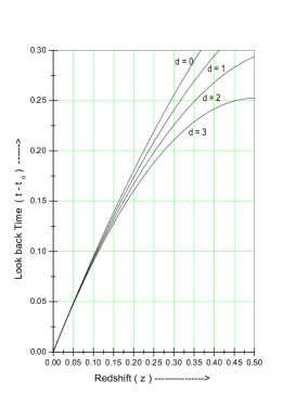
It follows from above that for a fixed z the look back time decreases with number of dimensions as evident from figure 7. Again it is shown that the look back time also increases with red shift (for small value of z).

6. Cosmological model with constant $\Lambda$ :

For the sake of completeness as also of relevance to the current accelerating scenario we briefly discuss in this section an earlier work of one of us with a constant $\Lambda$ [7]. In this work we discussed first zero pressure inhomogeneous 5D model with a constant $\Lambda$ and later generalized it to a fluid obeying an equation of state $p=m\rho\neq p_{5}$ where p is the isotropic three pressure, $p_{5}$ is the pressure in the fifth dimension, $\rho$ is the matter density and $m$ is a constant. At this stage it will not be out of place to point out that our set of solutions in Section 2 does not automatically reduce to the above mentioned works with a constant $\Lambda$ as our ansatz $\Lambda=kH^{2}$ in the present work does not permit that type of reduction.

For the line element (1) with d=1 ( 5D space time) and $\Lambda$ = constant we get for the matter dominated case ($p=p_{d}=0$)

$$a=a_{0}\sinh^{\frac{1}{2}}pt$$ (37)

$$b=\frac{(b_{0}-cr^{2})\sinh pt+b_{1}\cosh pt+\frac{4c}{p^{2}}}{\sinh^{\frac{1}{2}}pt}$$ (38)

$p=\sqrt{\frac{2\Lambda}{3}}$, where ($a_{0},b_{0},b_{1}$ are arbitrary constants, and c is the usual 4D curvature in the t-constant hypersurface.

To facilitate comparison with our homogeneous space of section (3) we put c = 0 such that the line element read

$$a=a_{0}\sinh^{\frac{1}{2}}pt;~{}~{}~{}~{}b=\frac{b_{0}\sinh pt+b_{1}\cosh pt}{\sinh^{\frac{1}{2}}pt}$$ (39)

Following [27] we, at this stage, define a deceleration parameter such that an affective ‘scale factor’ L becomes

$$L=(a^{3}b)^{\frac{1}{4}}=\sinh^{\frac{1}{4}}pt(\sinh pt+\cosh pt)^{\frac{1}{4}}$$ (40)

( putting $a_{0},b_{0},b_{1}$ unity, for simplicity). The well known 4D deceleration parameter ( say $q_{1}$ ) in this formalism becomes

$$q_{1}=-\frac{\ddot{L}L}{\dot{L}^{2}}=-8\sinh pt\cosh pt+8\cosh^{2}pt-5$$ (41)

The behaviour of $q_{1}$ here is interesting. At the early epoch the last expression shows that $q_{1}>0$ ( good news for structure formations ).

The flip occurs at the instant $t=t_{0}$, then the universe starts acceleration in conformity with the present day observation. It should, however, be emphasized that any attempt to compare the flip time of our model given above with observational findings will be too ambitions due to several initial assumptions in solving the equations as also due to the presence of so many arbitrary constants. One may, however, fine tune the arbitrary constants to account for the current observations.

If we further assume $b_{1}=0$ we get isotropic expansion , i.e. , $a=b$. In this case the expression for q ( say $q_{2}$) turns out to be

$$q_{2}=-\frac{\cosh^{2}pt-2}{\cosh^{2}pt}$$ (42)

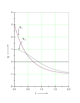
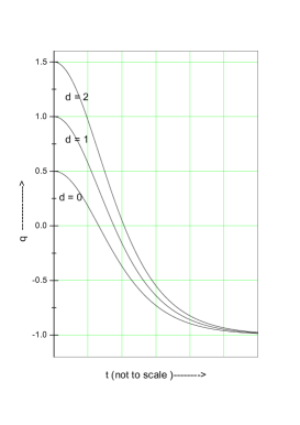
From the expression (41) and (42) it is evident that the flip occurs earlier for the anisotropic case, which is also evident from our figure 8. However the cosmological implications of this finding need further investigation.

Figure 8: The time evolution (t not to scale) of q is shown in this figure. It is shown that flip for $q_{1}$ is earlier than flip for $q_{2}$.

To end the section let us find out if the presence of extra dimensions, in any way, influences the instant of flip for the isotropic case. From the divergence equation in (3+d+1)-dimensional homogeneous space time for line element (1), we get,

$$\dot{\rho}+\left(3\frac{\dot{a}}{a}+d\frac{\dot{b}}{b}\right)\left(\rho+p\right)=0$$ (43)

which for our case ($p=0,~{}a=b$) yields

$$\rho=Ca^{-(d+3)}$$ (44)

Using equation (44) in equation (19), we get

$$\frac{\dot{a}^{2}}{a^{2}}=\frac{2}{(d+2)(d+3)}\left[\Lambda+Ca^{-(d+3)}\right]$$ (45)

Skipping mathematical details and adjusting the arbitrary constant $C$ we finally get from equation (45 )

$$a=a_{0}\sinh^{\frac{2}{d+3}}pt$$ (46)

where $p=\sqrt{\frac{d+3}{d+2}\Lambda}$. So the deceleration parameter reduces to

$$q=\frac{(d+3)-2\cosh^{2}pt}{2\cosh^{2}pt}$$ (47)

so the flip occurs at

$$\cosh pt_{c}=\sqrt{\frac{d+3}{2}}$$ (48)

Obviously the flip is delayed with the increasing of number of dimensions although a physical explanation of this behaviour is beyond the scope of the present investigations. Interestingly we got the same result in section 4 for the case of varying $\Lambda$ ( figure 9).

Figure 9: Flip is delayed with the number of dimensions

7. Discussion

In this work we have studied a multidimensional model (both homogeneous and inhomogeneous) with a time varying cosmological parameter. It is found that under certain conditions the cosmology gives an accelerated expansion. In the inhomogeneous case no initial deceleration is found. However for the homogeneous case an initially decelerating universe starts accelerating undergoing a flip.This is good for both structure formation and current observational status. Some of our cases are also amenable to the desirable feature of dimensional reduction. As mentioned earlier the dimensional reduction for our inhomogeneous model seemingly points to the fact that a primordial inhomogeneous higher dimensional cosmology enters a 4D homogeneous era although we do not have to make any stringent initial conditions to achieve this homogenization as tn the standard 4D case. This is an important finding of our analysis.While it is conjectured that the extra space stabilises at planckian length it is not apparent from our analysis how that mechanism in the form of a sort of repulsive potential field actually works in our model.This is definitely a defect of our model.However in an earlier work Guendelmann and Kaganovich[28] studied the Wheeler- Dewitt equation in the presence of a negative cosmological constant and dust and showed that quantum effects do stabilise the volume of the universe, thus providing a mechanism of quantum avoidance of the singularity. Other two important findings in our analysis are that the time of flip depends on the number of extra dimensions. In fact as the number of dimensions increase the flip is delayed thus higher dimensional models allow more time for structure formation. Secondly the flip also depends on anisotropy. Shear simply hastens the arrival of the instant of flip. It is too premature to attempt a physical explanation of the above two results but the results are interesting enough to warrant further investigations in this regard. To end a final remark is in order. We mentioned in the introduction that both extra dimensions and inhomogeneities produce a set of extra terms to the 4D FRW model, which creates a sort of back reaction [12] in the process. While the effect of extra dimension is discussed here in some detail, the influence of inhomogeneities in higher dimensional model will be discussed in our future work.
To end a final remark may be in order. We have here presented results which include cases when the extra dimensions also inflate along with the ordinary ones in section 3. While the idea of large extra dimensions is not as repugnant these days as in the past following its new found relevance in brane models but an inflating extra dimension goes far beyond that.This is a serious shortcoming of the present analysis, particularly the form of the spacetime we chose in section 3. While working in higher dimensional spacetime one should see that the extra space should form a compact manifold with the symmetry group G so that the $(d+3)$ spatial symmetry group is a direct product $O(3)\times G$ and not $O(d+3)$, although there exists a good number of works in this type of space also.

Acknowledgment : We acknowledge the financial support of UGC, New Delhi as also valuable comments of the anonymous referee.

References

- [1] Turner, M. S. Dark matter and dark energy : the critical questions, astro-ph/0207297.
- [2] Perlmutter, S. et al., (1999). Astro. Phys. J. 517, 565.
- [3] Randall, L., and Sundrum, R. (1999). Phys. Rev. Lett. 83, 3370.
- [4] Wesson, P. S., (1999). Space-Time-Matter, World Scientific.
- [5] Chatterjee, S., Banerjee, A., and Zhang, Y. Z. (2006). Int. J. Mod. Phys. A21, 4035 ; Panigrahi, D., Chatterjee, S., and Zhang, Y. Z., (2006). Int. J. Mod. Phys. A216491.
- [6] Je-An Gu, A way to the dark side of the universe through extra dimensions, astro-ph/0209223.
- [7] Chaterjee, S., Bhui, B., Barua, Basu, Madhumita, and Banerjee, A.,(1994). Phys. Rev. D50, 2924 ; Banerjee, A., Panigrahi, D., and Chatterjee, S., (1995). J. Math Phys. 36, 331.
- [8] Tosa, Y., (1984). Phys. Rev. D30, 2054.
- [9] Viswakarma, R. G., (2000). Class. Quantum Grav. 17, 3833.
- [10] Mustapha, N., Hellaby, C., and Ellis, G. F. R., (1997). Mon. Not. Royal Astro. 292, 817.
- [11] Russ, H., Soffel, M. H., Kasai, M., and Borner, G., (1997). Phys. Rev. D56, 2044.
- [12] Enqvist, Kari, and Mattsson, Teppo, J. Cosmol. Astropart. Phys. JCAP02(2007)019 and references therein.
- [13] Rasanen, S., J. Cosmol. Astropart. Phys. JCAP11(2006)003.
- [14] Kai, T., Kozaki, H., Nakao, K. i., Nambu, Y., and Yoo, C. M., Can inhomogeneities accelerate the cosmic volume expansion ?, gr-qc/0605120.
- [15] Lima, J. A. S., and Carvalho, J. C., (1994). Gen. Relativity Grav. 26, 909.
- [16] Arab, A. I., (1997). Gen. Relativity Grav. 29, 61.
- [17] Padmanabhan, T. Dark Energy: Mystry of the Millennium and references therein, astro-ph /0603114.
- [18] Overduim, J. M., Cooperstock, F. I., (1998). Phys. Rev. D58, 43506.
- [19] Chatterjee, S., Banerjee, A., (1993). Class. Quantum Grav. 10, L1.
- [20] Banerjee, A., Panigrahi, D., and Chatterjee, S. (1994). Class. Quantum Grav. 11, 1405.
- [21] Chodos, A., and Detweiler, S., (1980). Phys. Rev. D21, 2167.
- [22] Grøn, O., (1988). Astronomy Ashtrophysics 193, 1.
- [23] Ray, Saibal, and Mukhopadhyay, Utpal, (2007). Gravitation and Cosmology 13, 142.
- [24] Viswakarma, R. G., (2002). Class. Quantum Grav. 19, 4747.
- [25] Cayrel, R. et al., (2001). Nature 409, 691.
- [26] Narlikar, J. V., An Introduction to Cosmology, Cambridge University Press ( 3rd Edition)
- [27] Romano, Antonio, Enea, (2007). Phys. Rev. D75, 043509.
- [28] Guendelmann,E. and Kaganovich, A., (1993). Int. J. Mod. Phys. D 2, 221.
- [29] Sahdev, D., (1984). Phys. Lett. 137B, 155.