Nonlinear growth in modified gravity theories of dark energy
Abstract
Theoretical differences in the growth of structure offer the possibility that we might distinguish between modified gravity theories of dark energy and CDM. A significant impediment to applying current and prospective large scale galaxy and weak lensing surveys to this problem is that, while the mildly nonlinear regime is important, there is a lack of numerical simulations of nonlinear growth in modified gravity theories. A major question exists as to whether existing analytical fits, created using simulations of standard gravity, can be confidently applied. In this paper we address this, presenting results of N-body simulations of a variety of models where gravity is altered including the Dvali, Gabadadze and Porrati model. We consider modifications that alter the Poisson equation and also consider the presence of anisotropic shear stress that alters how particles respond to the gravitational potential gradient. We establish how well analytical fits of the matter power spectrum by Peacock and Dodds and Smith et al. are able to predict the nonlinear growth found in the simulations from up to today, and also consider implications for the weak lensing convergence power spectrum. We find that the analytical fits provide good agreement with the simulations, being within 1 of the simulation results for cases with and without anisotropic stress and for scale-dependent and independent modifications of the Poisson equation. No strong preference for either analytical fit is found.
I Introduction
A diverse range of observations are showing consistent evidence for the acceleration of the universe’s expansion, and the presence of dark energy, for example supernovae observations Riess et al. (2004); Astier et al. (2006); Riess et al. (2006), cosmic microwave background temperature and polarization fluctuations Spergel et al. (2006); Hinshaw et al. (2006); Jarosik et al. (2006); Page et al. (2006), large scale structure surveys Cole et al. (2005); Tegmark et al. (2006) and baryon acoustic oscillations Eisenstein et al. (2005).
Interpretation of Einstein’s cosmological constant as a vacuum energy requires the value to be fine-tuned to far smaller than any theoretical expectation, e.g.Carroll (2001)), and has forced the exploration of alternative theoretical explanations. Since precision measurements of gravity only exist for scales m (e.g.Adelberger et al. (2003)), there is freedom to posit modifications of gravity acting on larger scales, such as those in Dvali et al. (2000).
While cosmological observations of dark energy properties have so far focused on measurements of the homogeneous background density and astrophysical correlations in the linear regime, both theoretical and observational vistas are now opening up that require a good understanding of the growth of structure in the mildly nonlinear regime. Theoretically, measuring the growth of structure might enable modified gravity theories to be distinguished from a standard cosmological scenario (CDM) with a cosmological constant, , and cold dark matter (CDM) Linder and Cahn (2007); Amendola et al. (2007); Dore (2007). Observationally, the next generation of precision experiments will include weak lensing surveys, with several proposed large scale weak lensing experiments being developed in the coming decade, e.g. DUNE Refregier et al. (2006), JDEM/SNAP Albert et al. (2005) and LSST Tyson (2006).
Weak lensing is a potentially powerful probe of the late time evolution of the Universe, sensitive not only to the background expansion, but also able to give two-point and higher statistical correlations of the density field Takada and Jain (2004), potentially in tomographic redshift slices Jain and Taylor (2003); Bernstein and Jain (2004).
Modified gravity models can introduce extrinsic anisotropic shear stresses (see e.g. Bean et al. (2007)) that modify the relationship between the weak lensing potential and the matter over-density that might be detectable by contrasting weak lensing with other large scale structure observations Zhang et al. (2007); Amendola et al. (2007).
Many large scale structure statistics can be related to the underlying matter power spectrum, with nonlinear evolution at small scales. For standard general relativity, a typical approach is to use analytical fits based on N-body simulations of CDM Peacock and Dodds (1996); Smith et al. (2003) and CDM with dark energy with an equation of state,,CDM Ma et al. (1999); McDonald et al. (2006); Linder and White (2005) scenarios to apply the nonlinear correction to a linear power spectrum. Simulations of modified gravity models are for the most part lacking, however. With the exception of Stabenau and Jain (2006); Shirata et al. (2007), analyses often proceed by applying the CDM based analytical nonlinear fits to modified linear power spectra, e.g. Shirata et al. (2005); Amendola et al. (2007). Recently an analytical approach to estimating nonlinear growth in modified gravity, including those with anisotropic stress, Hu and Sawicki (2007a) was proposed and it was noted that there were currently no simulations against which to test the ansatz.
In this work we directly address to what degree the nonlinear fits developed for standard gravity can be utilized for modified gravity theories, and establish whether the paucity of simulations in modified gravity theories can be excused. We first consider the applicability of standard gravity nonlinear fits to modified gravity theories in which just the Poisson equation is modified, considering the 5D gravity form considered by Uzan and Bernardeau (2001), complementing the work of Stabenau and Jain (2006); Shirata et al. (2007) who considered nonlinear growth when a Yukawa-like gravitational coupling is introduced Sealfon et al. (2005). We then address the impact of anisotropic stress on nonlinear growth to assess if existing analytical nonlinear fits are adequate to model evolution in these scenarios. We consider the nonlinear growth in the Dvali, Gabadadze, and Porrati (DGP) 5D model Dvali et al. (2000) and in toy models that contrast the effects of anisotropic stress with those of a modified Poisson equation.
We first establish the framework for investigating modified gravity theories in Sec. II, and outline the specific models we consider with scale-independent and dependent modifications and the presence and absence of anisotropic shear. The details of our simulations and implementation, including the two standard analyitic fits are presented in Sec. III. The approach to weak lensing is discussed in Sec. IV. The results showing dimensionless power spectra and the success of analytic fits are discussed in Sec. V. An overview of the conclusions and implications of our results is then presented in Sec. VI.
II Modified Gravity Theories
We first outline the effect that the general modifications to gravity we study have on the perturbed Einstein’s equations. Following the notation of Ma and Bertschinger (1995), in the conformal Newtonian (or longitudinal) gauge, the metric is written as
| (1) |
where is the expansion factor, is the conformal time, is the comoving coordinate (=1,2,3 spatial directions) and and are the two gravitational metric perturbations.
Einstein’s equations relate the metric perturbations to fractional perturbations in density, , peculiar velocity, , and intrinsic shear for a matter component “”,
| (2) | |||||
| (3) | |||||
| (4) |
where , is the fractional energy density, and is the equation of state for the fluid. We have introduced the function as a modification in the relationship between the gravitational potentials and matter density in the equation, (2), and as an extrinsic anisotropic stress in addition to the intrinsic anisotropic stresses from the matter components (predominantly radiation) in the equation for , , (4). For standard gravity and .
Equations (2) and (3) combine to give
| (5) | |||||
| (6) |
where is a gauge invariant density variable defined in the rest frame of the matter components Kodama and Sasaki (1984).
Density and velocity perturbations evolve according to the perturbed fluid equations which are unchanged by the gravitational modifications,
| (7) | |||||
| (8) | |||||
where is the sound speed for the fluid.
We will consider a Universe dominated by pressureless matter, , and scenarios in which , so that on subhorizon scales , and
| (9) |
Using (8), we define the peculiar acceleration, ,
| (10) |
Following the notation of Amendola et al. (2007), we relate the anisotropic stress to through a function ,
| (11) |
and here are equivalent to and in Tsujikawa (2007).
Making a subhorizon approximation, and , assuming , the modified Poisson equation and peculiar acceleration equations are
| (12) | |||||
| (13) |
while the matter perturbation equation is
| (14) |
Note that, we can describe the evolution of in terms of the linear growth factor, , with respect to some reference scale, , where is scale-independent for standard gravity, but could be scale-dependent if gravity is so modified.
We can relate the Fourier space modification to a real space interaction in the form of a Green’s function,
| (15) | |||||
| (16) |
with recovering standard gravity. Using the convolution theorem we find,
| (17) |
The effect of modified gravity in weak lensing statistics is described in Schimd et al. (2005) where they show that the weak lensing distortion is dependent upon the sum of the two gravitational potentials, . As in Amendola et al. (2007), we introduce the parameter to describe the deviation of the weak lensing potential from standard gravity
| (18) | |||||
| (19) |
with for standard gravity.
II.1 5D Gravity
We consider a model, motivated by 5-dimensional gravity theories in which gravity is Newtonian on small scales but modified on scales larger than a characteristic scale Gregory et al. (2000); Binetruy and Silk (2001); Uzan and Bernardeau (2001). This model is characterized by the form
| (20) |
and
| (21) | |||||
with .
We are principally interested in the effect that modifications to gravity could have on the transition from linear to nonlinear regime, typically occurring over comoving scales Mpc. For our analysis, therefore, we consider evolution for values of the parameter of Mpc, Mpc, and Mpc, which alters the behavior in the relevant scales. We do not consider here smaller values of the modification which would alter behavior in the wholly nonlinear regime. We leave it for future study to assess whether such changes are well modeled by analytical fits describing the properties of collapsed halos.
II.2 DGP
A physical model that serves as an excellent example of the effects of anisotropic shear is the Dvali, Gabadadze, and Porrati (DGP) model Dvali et al. (2000) that is based on 5D gravity, wherein at some large scale, (comparable to the horizon scale), gravity is sensitive to the presence of an additional dimension.
The extra dimension alters the 4D background evolution to that described by the modified Friedmann equation,
| (22) |
where , with late time acceleration being triggered when the Universe’s horizon .
The modification also alters the growth of fluctuations in density and motion of matter. As well as a modification to the Poisson equation as discussed in Sec. II.1, this model also results in an anisotropic shear such that the two potentials are given by Lue et al. (2004); Koyama and Maartens (2006); Maartens and Majerotto (2006); Amendola et al. (2007):
| (23) | |||||
| (24) |
where
| (25) |
In contrast to Sec. II.1, this gives a scale-independent modification to the Poisson equation,
| (26) |
and nonnegligible anisotropic stress,
| (27) |
and .
II.3 Twin toy models
Finally, we consider a set of twin models that provide a simple way to further explore the effects of anisotropic stress on nonlinear growth. We consider two different modifications that both yield the same form for the weak lensing potential, with , such that they reduce to standard gravity at early times and become modified at late times. This form of is equivalent to model GDE1 of Amendola et al. (2007). The twin models (“TM”) we study have two contrasting, simple forms in terms of and :
| (28) |
and
| (29) |
In TM1, the Poisson equation is the same as for standard gravity; however, the peculiar acceleration of the matter particles responding to the gradient of the potential is affected by the anisotropic stress. In TM2, in contrast, the peculiar acceleration is the same as for standard gravity but the gravitational potential at late times has a different relation to matter over/under densities. We consider values of consistent with 1 and 2 Fisher-matrix constraints for a prospective DUNE-like weak lensing survey Amendola et al. (2007).
III N-Body Simulations
To obtain fully nonlinear results in each of the models, we obtain N-body simulations via a particle mesh(PM) code, taking as an initial form the code of Klypin and Holtzman (1997). For scale-independent modifications we make simple modifications to the code, described in Sec. III.1. For scale-dependent modifications we have to alter the potential and motion calculations as described in Sec. III.2.
III.1 Standard Gravity and Scale-independent Modifications
The PM code is reviewed in detail in Klypin and Holtzman (1997) but we provide some highlights in order to set the framework for discussing the modifications we make to the code.
PM codes operate by defining a simulation area as a box of size on a side, assuming it is closed so that we have periodic boundary conditions, subdividing it into a mesh or grid of cells (of size on a side), and defining all quantities on that mesh. The simulation is then initialized at some early redshift () and particles are placed according to model-dependent power spectra fits provided with the code (based on the cosmological parameters: the scalar spectral index ; the amplitude of fluctuations in 8 Mpc, ; the fractional density from curvature, , baryons, and cold dark matter, ; and the Hubble constant km s-1 Mpc-1). The evolution is then carried out by advancing time in equal steps of the expansion factor, . At each step in expansion factor the code determines a density in each cell, uses that density to compute the potential in each cell, and finally moves particles according to the gradient of the potential.
III.1.1 Defining the Density
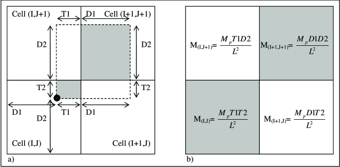
Defining the density can be done in a variety of ways; the code uses the cloud-in-cell scheme depicted in Fig. 1 wherein a particle is taken to be a cube with dimensions equal to that of the cells and with a corner positioned at the location of the particle. The particle contributes to each cell it extends into a mass equal to the particle’s total mass weighted by the fraction of the particle’s volume in the cell under consideration. Once the mass in each cell is determined it is effectively smeared over the entire cell.
III.1.2 Obtaining the Potential
For standard gravity, the code uses (12) with , with the dimensionless variables of Klypin and Holtzman (1997), and and writing ,
| (30) |
To evaluate (30), we use the discretized Poisson equation over cells, . In one dimension, the discrete Laplacian is given by
| (31) |
Defining the discrete Fourier transform,
| (32) |
the discretized Poisson equation is
| (33) |
Generalizing to three dimensions one obtains the ‘7-point crest template’,
| (34) | |||||
with
where is given by
| (35) |
Combining (III.1.2) and (30) the Poisson equation used in the code is,
| (36) |
The code calculates , Fourier transforms to , divides by and then transforms back to real space to obtain .
In the case of scale-indepedent modifications (36) is purely modified by
| (37) |
III.1.3 Advancing the Particles
Once we have the potential we advance the particles according to (16). In standard gravity, component wise on the grid we have only to compute
In the presence of anisotropic stress modifications,
| (38) |
III.2 Scale-dependent Modifications
In order to incorporate the scale-dependent modifications to gravity we follow the convolution approach in (15). To do this we multiply by at each step in rather than .
III.2.1 Defining the Radius for
In scale-dependent theories, by definition, we now convolve with functions involving the actual scale , and we must therefore define explicitly a radius on the grid. The mass is smeared over the entire cell it lies in, so that the distances simply become those between cells. The Fourier transforms involve periodic boundary conditions, so we define the radius for one origin at , and wrap the radius around the grid. Since the code uses the dimensionless radii to compute the function we have called , the cell indices can be used to construct the radius and we define to be the index of the relevant cell in the direction (=1,3).
The periodic boundary conditions require a change to the basic prescription presented above, namely to include the periodic boundary condition we must set up a 1D radius of the form where is the number of cells making up the grid in a dimension. Thus, the radii in the i-th dimension can be defined as
| (41) |
The final 3-dimensional radius, , is computed trivially as
| (42) |
There remains one final subtlety in computing the radius. Since , division by requires us to make a change to avoid infinities. To avoid these singularities we take the standard approach of ‘softening’ (e. g. Hockney and Eastwood (1989)), that is adding a small non-zero term to all the values of used in operations that would give a singularity. For instance if we consider we instead compute . Note that, for consistency, all values of r in the division are softened, not only the actual one that gives a singularity (). Further, note in the case of well defined modifications, e.g. the exponent need not be softened, so that we compute .
III.3 Obtaining Analytic Spectra
We compare the nonlinear spectra from simulations to predicted spectra from analytical mappings of linear power spectra using the Peacock and Dodds (PD) fit Peacock and Dodds (1996) and the Smith et al. fit (SP) Smith et al. (2003).
III.3.1 Analytical Linear Spectra
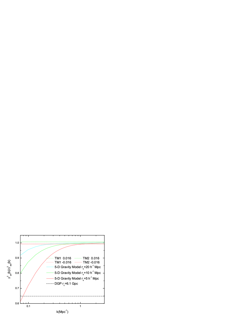
We evolve a linear CDM power spectrum obtained with CAMB Lewis and Bridle (2002) (that includes effects from baryon photon coupling at early times) forward in time using the modified equation for the growth of the over-density (14). We start at an epoch, we choose , at which the modification scale is large compared to the physical horizon, so that standard gravity is effectively recovered on the relevant scales, and evolve the density perturbations through the modified gravity era to today. In Fig. 2 we show the linear power spectra for the models discussed in the paper.
III.3.2 Analytical Non-Linear Fits
We briefly review the physical ingredients of the PD Peacock and Dodds (1996) and SP Smith et al. (2003) analytical fits against which we compare the simulations.
The PD fit is based on the assumption of stable clustering Davis and Peebles (1977), the hypothesis that the correlation function on scales smaller than those of virialized structures decouple from the expansion. The fit utilizes a linear to nonlinear mapping proposed by Hamilton et al. (HKML) Hamilton et al. (1991)
| (43) |
derived from the spherical collapse model. Peacock and Dodds generalized the HKML method to estimate the resulting nonlinear power spectrum through a universal scaling relation, ,
| (44) | |||||
| (45) |
where . The fitting function tends to in the linear limit, , and in the small scale, stable clustering limit, . There are five free parameters fit from N-body simulations in standard gravity as functions of the linear spectral index : and parameterize the power law in the quasilinear, large scale regime, parameterizes the amplitude of the in the stable clustering limit, describes the second order deviation from linear growth and softens the transition between the linear and fully virialized regimes. The cosmological model only enters into the fit through , consistent with the Zel’dovich approximation in which the final positions of particles are obtained by extrapolating their initial comoving displacements, , using the linear growth factor, .
The quality of the PD fit is founded on the broad applicability of the Zel’dovich approximation. However, with a scale-dependent modification of gravity, or the introduction of a difference between and it is not clear a priori how well the Zel’dovich approximation will apply, and if applicable, whether the numerical values of the coefficients will remain the same as those for standard gravity. That is, with scale-dependent modifications the possibility for shell crossings arises which causes a break down of the Zel’dovich approximation.
Looking at the functional form of the fit, in particular, we can consider three regimes to make predictions, namely, the large and small scale limits and a transition regime. Large scales which remain linear or quasilinear should be well described by the existing fit. On these scales the Zel’dovich approximation should hold and using a linear growth factor for is acceptable. Similarly and might be expected to adapt to the changed input power via their spectral index dependence, since in linear scales essentially all the information is contained in the amplitude and spectral index of the power spectrum.
The mildly nonlinear or transition regime, where we directly compare results, is particularly of interest in applying the fits. Scale-dependent modifications introduce an extra degree of freedom to growth in the model, a scale dependency that could also affect the shape and scale of the smoothing function interpolating between the linear and nonlinear asymptotic behaviors, essentially requiring corrections to . For example, a scale- or time-dependent modification to Poisson’s equation could alter the critical over-density required for nonlinear collapse, thus altering the details of the transition from linear to nonlinear regimes.
Small scale modifications to gravity, which we do not consider here, could well lead to alterations in the correlation function of the collapsed structures, in particular, changes to the value of the virialized normailzation . One might expect the application of the linear growth factor in the fit to be less effective even if including the linear scale dependency . Relevant to our analysis is the fact that the stable clustering approximation does not account for merging and accretion of halos and hence does not address how modifications to gravity may alter these physical processes. We discuss this in the context of the SP fit below.
The SP fit arises from a different approach based on the “halo model” Seljak (2000); Peacock and Smith (2000) in which the continuous accretion of matter and merging of halos is accounted for, deviating away from the stable clustering approximation. In this scenario, the power spectrum of matter is described on large scales by the correlations between different halos represented by a quasilinear term, , and on small scales by a halo term, , that accounts for power from the self-correlation of halos. In the fit, the two terms are phenomenologically selected functions of , where the scale becomes nonlinear at scale factor ,
| (46) | |||||
| (47) | |||||
is determined by the standard error of the linear density field,
| (48) | |||||
| (49) |
The eight coefficients {}, fit with spectral index-dependent functions, and three -dependent functions, , , and , are empirically matched to standard gravity simulations.
In the large scale limit, the quasilinear term dominates and the use of the spectral index dependent and suggest the fit will adapt well to a modification on linear scales, such as those considered here.
On small scales, just as in the PD case, there are issues with the numerical fitting functions in the halo self-correlation term; the correlation coefficient in a virialized halo could be modified for the various modified gravity scenarios. The functions , , and , which in standard gravity are purely functions of , would be expected to alter to account for the modification; this in turn could well be expected to change , , .
Also as in the PD case, the interpolation from linear to nonlinear regimes, from large to small scales, could be altered as the modifications could alter the critical over-density required for nonlinear collapse. In particular the form of and to some extent may be expected to require changes as these serve to determine the relative importance of the halo-halo and self-correlation terms.
It is in light of these considerations that we study whether these analytic fits can readily describe modified gravity scenarios, with scale-dependent or independent modifications to the Poisson equation, and/or scale-independent anisotropic shear.
IV Obtaining Weak Lensing Spectra
Modified gravity theories can impact weak lensing convergence power spectrum in addition to the matter power spectrum, thus we study the impact of our models on both. In standard gravity, the power spectrum of the convergence is given by
| (50) |
where is the matter power spectrum and is a weighting function that can be related to the comoving distance and the distribution of background or source galaxies,
| (51) |
We assume a a simple delta function distribution of sources at , so,
| (52) |
The convergence power spectrum is then
| (53) |
with
| (54) |
Where we have used the fact that the comoving distance, , is equal to the (comoving) angular diameter distance for a flat Universe so that
| (55) |
Gravitational modifications and/or , will act to modify . In addition, and/or will modify how the convergence spectrum is related to (see for example Amendola et al. (2007)), resulting in
| (56) | |||||
where the evolution of is also affected by and .
can be obtained from either the PM simulations or the analytic fits described in Sec. III.3. To actually evaluate the integral, we discretize it, binning by expansion factor.
When considering the N-body code derived , we have to account for the fact that the simulation only probes a range of , yet for any given , can can lie outside this range at some redshift, . For the range we consider, the range of needed is virtually all given by the N-body simulation. Outside this range, on large scales the power spectrum is well approximated by the linear spectrum; at smaller scales we find that the analytic SP and PD predictions for the modified gravity spectra are within the errors at the edges of the range of provided by the simulations, so we pad the simulated spectra with the nonlinear analytic fits to modified gravity linear power spectrum.
V Results
V.1 Parameters for Simulations
For the PM code parameters we take Mpc, and for our cosmological model we take , and . The resulting simulations measure scales Mpc-1. The specific choice of initial redshift is not important other than to ensure that it is early enough that nonlinear corrections are negligible.
The box size and number of cells play into spatial resolution of the simulation, and are chosen to allow us to effectively probe the decade of in which the mildly nonlinear effects manifest themselves and from which we can extract a reasonable weak lensing spectrum for , a range relevant to upcoming experiments. The number of particles are chosen to ensure a sufficient particle resolution for the box size and number of cells used.
The initial positions of the particles at , are assigned by means of a random number generator consistent with the initial power spectrum. Depending on the seed used to initialize the random number generator, the resultant spectra may agree well with standard CDM analytic fits with the same parameters or might over- or under-produce power, even in the original unaltered code of Klypin and Holtzman (1997). We therefore run the simulations with 24 random seeds to get a good sample size and a more robust average. In order to weight the behavior of each simulation equally, we consider the modifications in terms of the “average of the ratios” of the modified power spectrum to the standard gravity spectrum for the same seed, rather than the “ratio of the averages” that would preferentially weight those simulations that over-produce power.
For scale-dependent modified gravity, we find the Numerical Recipes routine Press et al. (2007) for the Fourier transform, though slightly more time consuming, is more stable than the one provided in the original code. In the case of scale-independent modifications and standard gravity, both algorithms produce identical results. The softening parameter value used for the scale-dependent modification is much smaller than the smallest separation in the code and provides agreement with standard gravity from analytic predictions and standard gravity simulations with the code at least at the level or better than the unmodified Klypin code.

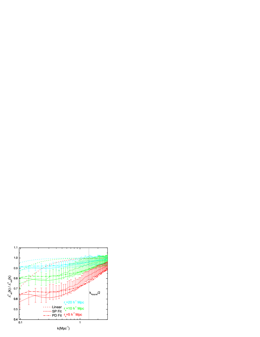
In Fig. 3 we show the results of the 24 simulations of standard gravity against the SP and PD fits, in order to demonstrate the fiducial model against which the modified gravity simulations are compared. The simulations are consistent with the analytical fits in the range Mpc Mpc-1. A conservative estimate for the largest at which we can believe the simulation results are reasonable is Stabenau and Jain (2006), which for our simulations is Mpc-1. We consider the simulations to be valid only up to , rather than up to as this more conservative limit represents a regime in which standard gravity simulations and fits agree to within 1.5 times the standard error in the simulation, in comparison to 10 (for the PD fit) and 13 (for the SP fit) times the standard error at .
For the model parameterizations we consider, we find that the linear scales used to generate the nonlinear in the range Mpc-1 lie in the range Mpc-1.
V.2 Simulation and Analytic Fit Results
V.2.1 5D Gravity Model
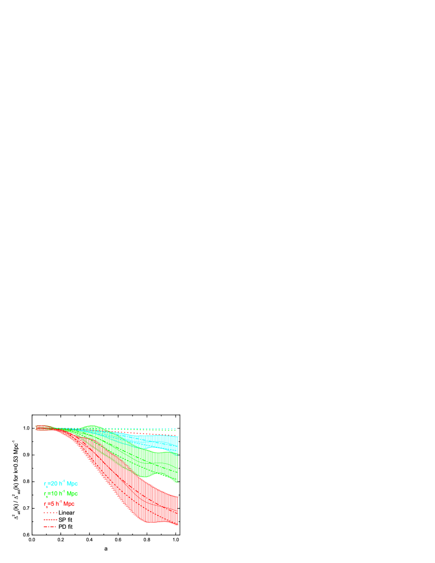
The ratio of the dimensionless power spectrum today for the 5D gravity model discussed in Sec. II.1 to standard gravity, is shown in Fig. 4. We find that the simulations are consistent with the PD Peacock and Dodds (1996) fit at the level. This is consistent with the results of Stabenau and Jain (2006) for a Yukawa type modification (that, like the modification we consider here, is a scale-dependent modification). The SP fits are slightly less consistent with the numerical predictions, however, still lie within 1 of the simulation mean. We, therefore, find no statistical basis for preferring PD over the SP Smith et al. (2003) fit of .
To consider the suitability of the analytic fitting functions when applied to weak lensing, it is insufficient to purely consider their agreement with predictions today; the entire evolution must be tracked between the redshift of the lensed source and today, as weak lensing integrates over the expansion factor , c.f. (56). We, therefore, track the redshift history of the nonlinear evolution, and the comparison with the analytical fits, as shown in Fig. 5. We find both fits lie within 1 though after the SP results are just encompassed by the 1 errors.
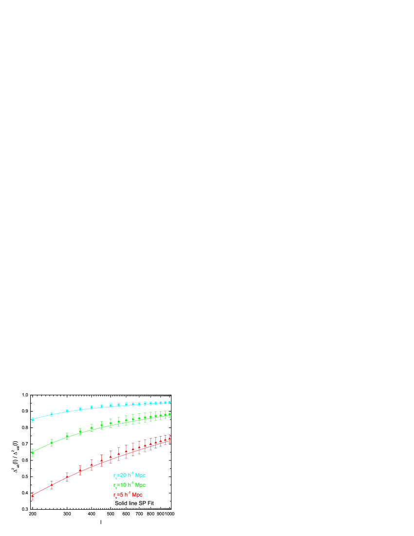
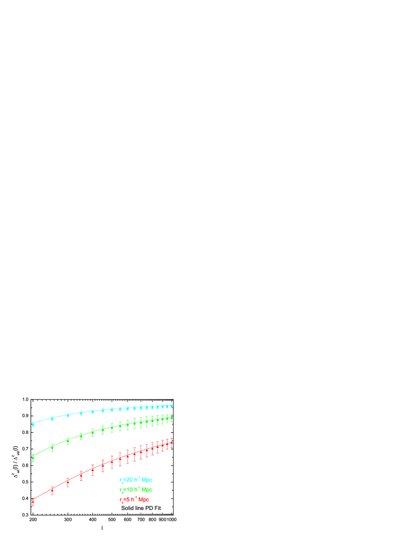
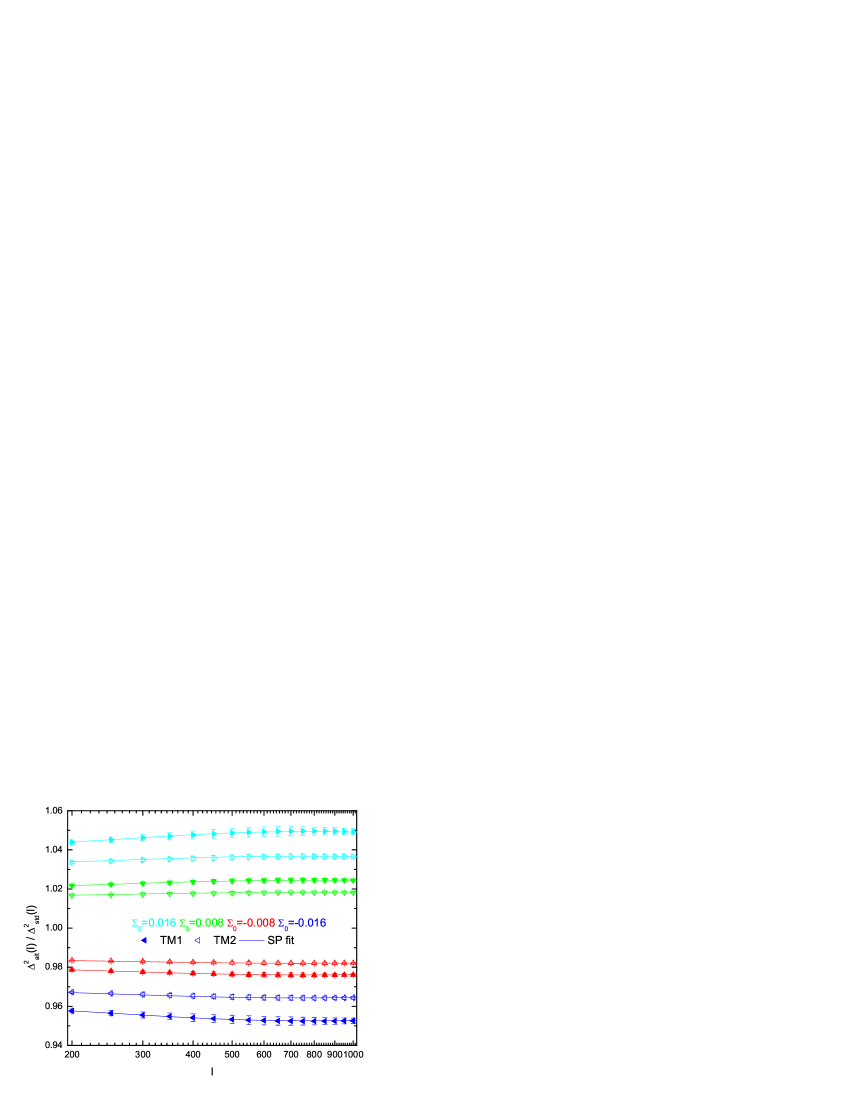
The ratios of the modified gravity weak lensing spectra to those of standard gravity are well recovered by the PD and SP fits, as shown in Fig. 6. The ratios of the weak lensing convergence spectra are slightly less sensitive to the exact form of the modification than the matter power spectra, for two reasons. First, the integral in (56) is mostly weighted towards integrand values at early times when the analytical fits are in very strong agreement with the simulations. Thus, for instance, the late-time transition of the SP fit to the outer regions of the 1-sigma level is not so significant to the convergence power as it is to the final matter power spectrum. Secondly, we “pad” the spectrum at values outside the simulated range with the analytical fit, in order to evaluate in (56). This is mitigated (as discussed in Sec. IV) by the similarity of the fits and the code spectra at the edges of our range of and the fact that the contribution from padded values is small in comparison to those drawn from the simulated range: for , is padded with the nonlinear analytical spectrum at , which corresponds to 1.3% of for standard gravity; for the padding is required for which contributes to 14% of the value of .
V.2.2 DGP
The effects of nonlinear growth in DGP models are of great interest in establishing observational distinctions between this model and standard CDM at cosmological scales, in Amendola et al. (2007) the nonlinear power spectrum was estimated using the Smith et al. analytical fit, while in Hu and Sawicki (2007a) an analytical ansatz is applied. Both the DGP model and the model in Sec. II.1 are motivated by 5D modifications to gravity. The difference between DGP and that model is that DGP not only modifies the Poisson equation but also the peculiar acceleration through the presence of an anisotropic stress.
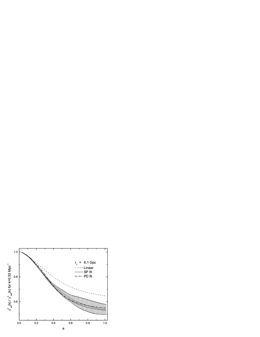
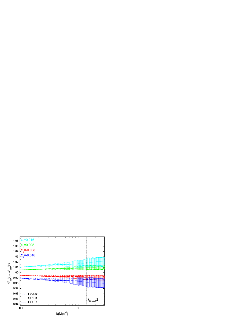
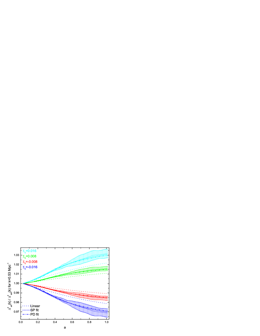
For the arguably more complex DGP model, the SP and PD fits are both still in good agreement with the N-body simulations at , at the 1 level over the simulated scales, as shown in Fig. 7. This is also true over the course of the evolution as the modification from CDM switches on, as shown in Fig. 8.
Note that we do not provide a weak lensing analysis in this model; as due to the change in [and hence in ] evaluating consistently results in a need for much smaller scales, i.e. Mpc-1 for the range of ’s we have considered. We thus restrict our discussion of DGP to matter power spectra and their evolution.
Even though is chosen to be in close agreement with the background evolution of our fiducial cosmological model, and has essentially degenerate evolution at early times, the DGP model shows marked deviation from standard gravity at late times. We note that the suppression of the nonlinear power spectrum shown with respect to standard gravity for the PD and SP fits and N-body simulations is qualitatively similar to that shown with the ansatz of Hu and Sawicki (2007a), although we leave a quantitative assessment of the ansatz to future work.
V.2.3 Twin Toy Models
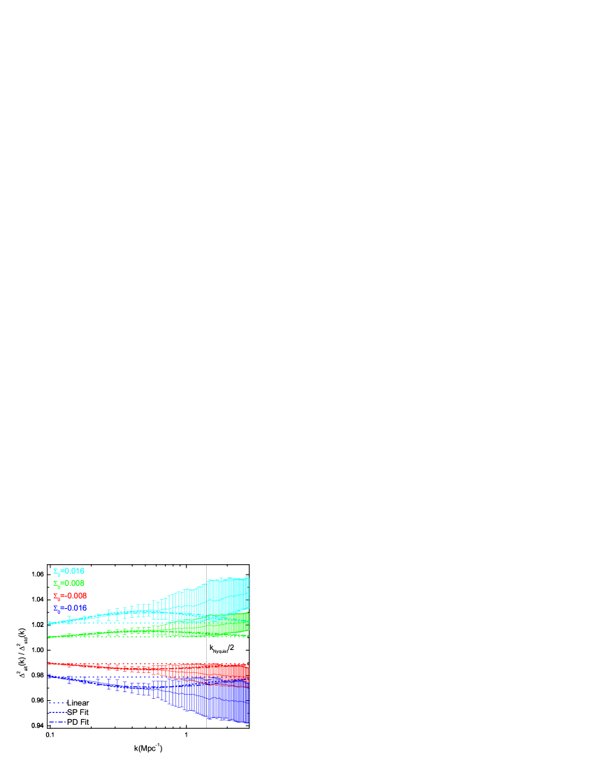
In order to investigate the abilities of the two analytical fits to predict nonlinear behavior in the two types of modifications, we consider a set of twin toy models, described in Sec. II.3. TM1 has a modified Poisson equation while TM2 has anisotropic stress . Both models have the same form of relationship of the weak lensing potential to the over-density, characterized by the function . As shown in Fig. 11, despite the degenerate background evolutions, the different modifications in each model lead to different linear scale-independent growth factors. For both models, the SP and PD analytical fits track both the scale-dependent behavior and time evolution of nonlinearities in both types of scenario, as shown in Figs. 9 and 10. The weak lensing correlations for PD and SP fits are virtually identical for each model so we only show the results for SP fits in Fig. 11; the difference between the simulations and analytical fits is negligible for both models.
V.3 Discussion
The nonlinear fits of Peacock and Dodds and Smith et al. have been shown to work across broad cosmological models with standard gravity, with different fractional mass densities, curvature, and initial power spectrum spectral indices. The utility of these fits derives from the wide applicability of the Zel’dovich approximation. In both fits there is the conjecture that the statistics of the gravitational clustering obey a similarity transform for which no proof is given, but instead is experimentally shown to be robust for a variety of cosmological models by simulation. In this paper we assess whether such a similarity transform similarly exists in modified gravity theories, and moreover that the existing quantitative values for the fit coefficients can be used. This is not necessarily the case a priori.

To test the fits we have performed nonlinear simulations of models in which modifications to Poisson and the peculiar acceleration occur exactly in this mildly nonlinear, transition regime. We have found that both the SP and PD analytical fits give reasonably good agreement with the simulations, in spite of the scale- and time-dependent modifications. This implies that applicability of the Zel’dovich approximation extends to scenarios in which anisotropic stress and even those with scale-dependent modifications to gravity are present in the mildly nonlinear regime. The modifications, therefore, are well described by the fits through their impact on the linear growth factor, , and the spectral index dependency of the fitting functions. It appears that scale-dependent modifications in the mildly nonlinear regime do not require significant modification of the numerical coefficients in the fitting functions. Since our simulations focus on the ability of the fits to accurately match the transition from linear to nonlinear regimes, they do not investigate if modifications on small scales, in which the subhalo correlations are key, are well described by the fits, for example, if in (20) were significantly smaller, e.g. less than Mpc. This is an area of interest for further analysis, especially in recently discussed theories in which galactic scale modifications could be present (e.g. Hu and Sawicki (2007b)).

VI Conclusions
The use of complementary cosmological observations to probe the properties of dark energy has proved extremely powerful. Observations sensitive to the background evolution, e.g. supernovae, or the wholly linear regime, e.g. the cosmic microwave background, have been the major observational tools to constrain dark energy to date. There is now significant interest, however, in applying a broader range of observations including those sensitive to large scale structure including large scale galaxy surveys, such as the Sloan Digital Sky Survey, and current and prospective weak lensing surveys. For each of these, in order to make precise inferences about dark energy, theoretical systematic errors about the modeling of nonlinear corrections must be addressed.
This work considers the ability of the commonly used nonlinear analytical fits of Peacock and Dodds Peacock and Dodds (1996) and Smith et al. Smith et al. (2003) to predict nonlinear growth in a variety of theories beyond standard gravity. We consider models in which the Poisson equation is modified, based on 5D gravity, Gregory et al. (2000); Binetruy and Silk (2001); Uzan and Bernardeau (2001) and also those in which peculiar acceleration response to the gravitational potential is altered, including the DGP model Dvali et al. (2000).
We find that the two fitting functions provide robust predictions for theories with both types of modification, in terms of accurately predicting the matter power spectrum today, and also, vitally for calculating the weak lensing convergence spectrum, they predict the development of nonlinearities over time. Both consistently give predictions within 1 of 24 simulated N-body realizations of the theory. Our results imply that the similarity conjecture for mapping linear to nonlinear power empirically found to be satisfied in standard gravity simulations is also applicable to scenarios in which gravity has scale- and time-dependent modifications. This suggests that the spectral index dependence of the fitting function and the linear growth factor effectively describe alterations in the nonlinear collapse due to scale-dependent modifications to gravity and anisotropic stress at the scales studied in the models here.
We conclude that current analytic fits using the linear power spectrum in modified gravity theories can be used to accurately predict the nonlinear growth in theories with scale-independent or dependent modifications, and in those with or without anisotropic stress in the mildly nonlinear regime. We find no statistical evidence for a preference, on the basis of overall performance, for one analytical fit over the other.
Many modified gravity models, for example, DGP and models, exhibit gravitational modifications on subhalo scales. Whether such modifications are well described by the halo term in the SP fit or the stable clustering approximation in the PD fit necessitates smaller scale simulations in the substantially nonlinear regime, which lies outside the scope of this paper.
We have limited our investigation of anisotropic stress to scale-independent modifications, and indeed further work is warranted in investigating whether the conclusions found for those are applicable to scale-dependent anisotropic stress, as found in theories. It will also be interesting to investigate the agreement between simulations and the recently proposed nonlinear ansatz Hu and Sawicki (2007a) for modified gravity models.
Acknowledgments
We thank Anatoly Klypin and Jon Holtzman for kindly making their PM code publicly available and Olivier Dore, Hans Stabenau and Ira Wasserman for valuable discussions in the course of this work. The work of IL and RB is supported by the National Science Foundation under Grants No. AST-0607018 and No. PHY-0555216.
References
- Riess et al. (2004) A. G. Riess et al. (Supernova Search Team), Astrophys. J. 607, 665 (2004), eprint astro-ph/0402512.
- Astier et al. (2006) P. Astier et al., Astron. Astrophys. 447, 31 (2006), eprint astro-ph/0510447.
- Riess et al. (2006) A. G. Riess et al. (2006), eprint astro-ph/0611572.
- Spergel et al. (2006) D. N. Spergel et al. (2006), eprint astro-ph/0603449.
- Hinshaw et al. (2006) G. Hinshaw et al. (2006), eprint astro-ph/0603451.
- Jarosik et al. (2006) N. Jarosik et al. (2006), eprint astro-ph/0603452.
- Page et al. (2006) L. Page et al. (2006), eprint astro-ph/0603450.
- Cole et al. (2005) S. Cole et al. (The 2dFGRS), Mon. Not. Roy. Astron. Soc. 362, 505 (2005), eprint astro-ph/0501174.
- Tegmark et al. (2006) M. Tegmark et al., Phys. Rev. D74, 123507 (2006), eprint astro-ph/0608632.
- Eisenstein et al. (2005) D. J. Eisenstein et al. (SDSS), Astrophys. J. 633, 560 (2005), eprint astro-ph/0501171.
- Carroll (2001) S. M. Carroll, Living Rev. Rel. 4, 1 (2001), eprint astro-ph/0004075.
- Adelberger et al. (2003) E. G. Adelberger et al., Ann. Rev. Nucl. Part. Sci. 53, 77 (2003), eprint hep-ph/0307284.
- Dvali et al. (2000) G. R. Dvali, G. Gabadadze, and M. Porrati, Phys. Lett. B485, 208 (2000), eprint hep-th/0005016.
- Linder and Cahn (2007) E. V. Linder and R. N. Cahn (2007), eprint astro-ph/0701317.
- Amendola et al. (2007) L. Amendola, M. Kunz, and D. Sapone (2007), eprint arXiv:0704.2421 [astro-ph].
- Dore (2007) O. Dore (2007), eprint (unpublished).
- Refregier et al. (2006) A. Refregier et al. (2006), eprint astro-ph/0610062.
- Albert et al. (2005) J. Albert et al. (2005), eprint astro-ph/0507460.
- Tyson (2006) J. A. Tyson (LSST), AIP Conf. Proc. 870, 44 (2006), eprint astro-ph/0609516.
- Takada and Jain (2004) M. Takada and B. Jain, Mon. Not. Roy. Astron. Soc. 348, 897 (2004), eprint astro-ph/0310125.
- Jain and Taylor (2003) B. Jain and A. Taylor, Phys. Rev. Lett. 91, 141302 (2003), eprint astro-ph/0306046.
- Bernstein and Jain (2004) G. M. Bernstein and B. Jain, Astrophys. J. 600, 17 (2004), eprint astro-ph/0309332.
- Bean et al. (2007) R. Bean, D. Bernat, L. Pogosian, A. Silvestri, and M. Trodden, Phys. Rev. D75, 064020 (2007), eprint astro-ph/0611321.
- Zhang et al. (2007) P. Zhang et al. (2007), eprint arxiv:0704.1932[astro-ph].
- Peacock and Dodds (1996) J. A. Peacock and S. J. Dodds, Mon. Not. Roy. Astron. Soc 280, L19 (1996), eprint astro-ph/9603031.
- Smith et al. (2003) R. Smith et al., Mon. Not. Roy. Astron. Soc 341, 1311 (2003), eprint astro-ph/0207664.
- Ma et al. (1999) C.-P. Ma, R. R. Caldwell, P. Bode, and L.-M. Wang, Astrophys. J. 521, L1 (1999), eprint astro-ph/9906174.
- McDonald et al. (2006) P. McDonald, H. Trac, and C. Contaldi, Mon. Not. Roy. Astron. Soc. 366, 547 (2006), eprint astro-ph/0505565.
- Linder and White (2005) E. V. Linder and M. J. White, Phys. Rev. D72, 061304(R) (2005), eprint astro-ph/0508401.
- Stabenau and Jain (2006) H. F. Stabenau and B. Jain, Phys. Rev. D74, 084007 (2006), eprint astro-ph/0604038.
- Shirata et al. (2007) A. Shirata, Y. Suto, C. Hikage, T. Shiromizu, and N. Yoshida, Phys. Rev. D76, 044026 (2007), eprint arXiv:0705.1311 [astro-ph].
- Shirata et al. (2005) A. Shirata, T. Shiromizu, N. Yoshida, and Y. Suto, Phys. Rev. D71, 064030 (2005), eprint astro-ph/0501366.
- Hu and Sawicki (2007a) W. Hu and I. Sawicki (2007a), eprint arXiv:0708.1190 [astro-ph].
- Uzan and Bernardeau (2001) J.-P. Uzan and F. Bernardeau, Phys. Rev. D64, 083004 (2001), eprint hep-ph/0012011.
- Sealfon et al. (2005) C. Sealfon, L. Verde, and R. Jimenez, Phys. Rev. D71, 083004 (2005), eprint astro-ph/0404111.
- Ma and Bertschinger (1995) C.-P. Ma and E. Bertschinger, Astrophys. J. 455, 7 (1995), eprint astro-ph/9506072.
- Kodama and Sasaki (1984) H. Kodama and M. Sasaki, Prog. Theor. Phys. Suppl. 78, 1 (1984).
- Tsujikawa (2007) S. Tsujikawa, Phys. Rev. D76, 023514 (2007), eprint arXiv:0705.1032 [astro-ph].
- Schimd et al. (2005) C. Schimd, J.-P. Uzan, and A. Riazuelo, Phys. Rev. D71, 083512 (2005), eprint astro-ph/0412120.
- Gregory et al. (2000) R. Gregory, V. A. Rubakov, and S. M. Sibiryakov, Phys. Rev. Lett. 84, 5928 (2000), eprint hep-th/0002072.
- Binetruy and Silk (2001) P. Binetruy and J. Silk, Phys. Rev. Lett. 87, 031102 (2001), eprint astro-ph/0007452.
- Lue et al. (2004) A. Lue, R. Scoccimarro, and G. D. Starkman, Phys. Rev. D69, 124015 (2004), eprint astro-ph/0401515.
- Koyama and Maartens (2006) K. Koyama and R. Maartens, JCAP 0601, 016 (2006), eprint astro-ph/0511634.
- Maartens and Majerotto (2006) R. Maartens and E. Majerotto, Phys. Rev. D74, 023004 (2006), eprint astro-ph/0603353.
- Klypin and Holtzman (1997) A. Klypin and J. Holtzman (1997), eprint astro-ph/9712217.
- Hockney and Eastwood (1989) R. W. Hockney and J. W. Eastwood, Computer Simulation Using Particles (edited by Adam Hilger, IOP Publishing, Bristol, United Kingdom, 1989).
- Lewis and Bridle (2002) A. Lewis and S. Bridle, Phys. Rev. D66, 103511 (2002), eprint astro-ph/0205436.
- Davis and Peebles (1977) M. Davis and P. J. E. Peebles, Astrophys. J. Supplement Series 34, 425 (1977).
- Hamilton et al. (1991) A. Hamilton, P. Kumar, E. Lu, and A. Matthews, Astrophys. J. 374, L1 (1991).
- Seljak (2000) U. Seljak, Mon. Not. Roy. Astron. Soc. 318, 203 (2000).
- Peacock and Smith (2000) J. Peacock and R. Smith, Mon. Not. Roy. Astron. Soc. 318, 1144 (2000).
- Press et al. (2007) W. H. Press, S. A. Teukolsky, W. T. Vetterling, and B. P. Flannery, Numerical Recipes : The Art of Scientific Computing (Cambridge University Press, Cambridge, England, 2007).
- Hu and Sawicki (2007b) W. Hu and I. Sawicki, Phys. Rev. D76, 064004 (2007b), eprint arXiv:0705.1158 [astro-ph].