Navigability of complex networks

Abstract

Routing information through networks is a universal phenomenon in both natural and manmade complex systems. When each node has full knowledge of the global network connectivity, finding short communication paths is merely a matter of distributed computation. However, in many real networks nodes communicate efficiently even without such global intelligence. Here we show that the peculiar structural characteristics of many complex networks support efficient communication without global knowledge. We also describe a general mechanism that explains this connection between network structure and function. This mechanism relies on the presence of a metric space hidden behind an observable network. Our findings suggest that real networks in nature have underlying metric spaces that remain undiscovered. Their discovery would have practical applications ranging from routing in the Internet and searching social networks, to studying information flows in neural, gene regulatory networks, or signaling pathways.

I Introduction

Networks are ubiquitous in all domains of science and technology, and permeate many aspects of daily human life Albert and Barabási (2002); Newman (2003); Dorogovtsev and Mendes (2003); Boccaletti et al. (2006), especially upon the rise of the information technology society Castells (1996); Pastor-Satorras and Vespignani (2004). Our growing dependence on them has inspired a burst of activity in the new field of network science, keeping researchers motivated to solve the difficult challenges that networks offer. Among these, the relation between network structure and function is perhaps the most important and fundamental. Transport is one of the most common functions of networked systems. Examples can be found in many domains: transport of energy in metabolic networks, of mass in food webs, of people in transportation systems, of information in cell signalling processes, or of bytes across the Internet.

In many of these examples, routing –or signalling of information propagation paths through a complex network maze– plays a determinant role in the transport properties of the system, in particular in such systems as the Internet or airport networks that have transport as their primary function. The observed efficiency of this routing process in real networks poses an intriguing question: how is this efficiency achieved? When each element of the system has a full view of the global network topology, finding short routes to target destinations is a well-understood computational process. However, in many networks observed in nature, including those in society and biology (signalling pathways, neural networks, etc.), nodes efficiently find intended communication targets even though they do not possess any global view of the system. For example, neural networks would not function so well if they could not route specific signals to appropriate organs or muscles in the body, although no neurone has a full view of global inter-neurone connectivity in the brain.

In this work, we identify a general mechanism that explains routing conductivity, or navigability of real networks based on the concept of similarity between nodes Watts et al. (2002); Girvan and Newman (2002); Menczer (2002); Leicht et al. (2006); Crandall et al. (2008); Clauset et al. (2008). Specifically, intrinsic characteristics of nodes define a measure of similarity between them, which we abstract as a hidden distance. Taken together, hidden distances define a hidden metric space for a given network. Our recent work shows that these spaces explain the observed structural peculiarities of several real networks, in particular social and technological ones Ángeles Serrano et al. (2008). Here we show that this underlying metric structure can be used to guide the routing process, leading to efficient communication without global information in arbitrarily large networks. Our analysis reveals that, remarkably, real networks satisfy the topological conditions that maximise their navigability within this framework. Therefore, hidden metric spaces offer explanations of two open problems in complex networks science: the communication efficiency networks so often exhibit, and their unique structural characteristics.

II Node similarity and hidden metric spaces

Our work is inspired by the seminal work of sociologist Stanley Milgram on the small world problem. The small world paradigm refers to the existence of short chains of acquaintances among individuals in societies Travers and Milgram (1969). At Milgram’s time, direct proof of such a paradigm was impossible due to the lack of large databases of social contacts, so Milgram conceived an experiment to analyse the small world phenomenon in human social networks. Randomly chosen individuals in the United States were asked to route a letter to an unknown recipient using only friends or acquaintances that, according to their judgement, seemed most likely to know the intended recipient. The outcome of the experiment revealed that, without any global network knowledge, letters reached the target recipient using, on average, $5.2$ intermediate people, demonstrating that social acquaintance networks were indeed small worlds.

Figure 1: How hidden metric spaces influence the structure and function of complex networks. The smaller the distance between two nodes in the hidden metric space, the more likely they are connected in the observable network topology. If node $A$ is close to node $B$, and $B$ is close to $C$, then $A$ and $C$ are necessarily close because of the triangle inequality in the metric space. Therefore, triangle $ABC$ exists in the network topology with high probability, which explains the strong clustering observed in real complex networks. The hidden space also guides the greedy routing process: if node $A$ wants to reach node $F$, it checks the hidden distances between $F$ and its two neighbours $B$ and $C$. Distance $CF$ (green dashed line) is smaller than $BF$ (red dashed line), therefore $A$ forwards information to $C$. Node $C$ then performs similar calculations and selects its neighbour $D$ as the next hop on the path to $F$. Node $D$ is directly connected to $F$. The result is path $A\to C\to D\to F$ shown by green edges in the observable topology.

The small world property can be easily induced by adding a small number of random connections to a “large world” network Watts and Strogatz (1998). More striking is the fact that social networks are navigable without global information. Indeed, the only information that people used to make their routing decisions in Milgram’s experiment was a set of descriptive attributes of the destined recipient, such as place of living and occupation. People then determined who among their contacts was “socially closest” to the target. The success of the experiment indicates that social distances among individuals –even though they may be difficult to define mathematically– play a role in shaping the network architecture and that, at the same time, these distances can be used to navigate the network. However, it is not clear how this coupling between the structure and function of the network leads to efficiency of the search process, or what the minimum structural requirements are to facilitate such efficiency Kleinberg (2000a).

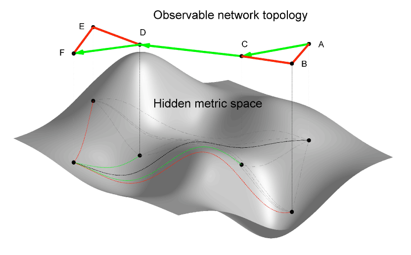
In this work, we show how network navigability depends on the structural parameters characterising the two most prominent and common properties of real complex networks: (1) scale-free (power-law) node degree distributions characterising the heterogeneity in the number of connections that different nodes have, and (2) clustering, a measure of the number of triangles in the network topology. We assume the existence of a hidden metric space, an underlying geometric frame that contains all nodes of the network, shapes its topology, and guides routing decisions, as illustrated in Fig. 1. Nodes are connected in the observable topology, but a full view of their global connectivity is not available at any node. Nodes are also positioned in the hidden metric space and identified by their co-ordinates in it. Distances between nodes in this space abstract their similarity Watts et al. (2002); Girvan and Newman (2002); Menczer (2002); Leicht et al. (2006); Crandall et al. (2008); Clauset et al. (2008). These distances influence both the observable topology and routing function: (1) the smaller the distance between two nodes in the hidden space, i.e., the more similar the two nodes, the more likely they are connected in the observable topology; (2) nodes also use hidden distances to select, as the next hop, the neighbour closest to the destination in the hidden space. Kleinberg introduced the term greedy routing to describe this forwarding process Kleinberg (2000a). Greedy routing and its modifications have been studied extensively in recent computer science literature Kleinberg (2000b, 2001); Manku et al. (2004); Martel (2004); Nguyen and Martel (2005, 2008); Simsek and Jensen (2005); Lebhar and Schabanel (2004); Fraigniaud (2005); Fraigniaud et al. (2006, 2007); Fraigniaud and Gavoille (2008); Chaintreau et al. (2008) (see also Kleinberg’s review Kleinberg (2006) and references therein). However, most of these works do not study greedy routing on scale-free topologies, which are known as the common signature of many large-scale self-evolving complex networks Albert and Barabási (2002); Newman (2003); Dorogovtsev and Mendes (2003).

We use the class of network models developed in recent work Ángeles Serrano et al. (2008). They generate networks with topologies similar to those of real networks –small-world, scale-free, and with strong clustering– and, simultaneously, with hidden metric spaces lying underneath. The simplest model in this class (the details are in Appendix A) uses a one-dimensional circle as the underlying metric space, in which nodes are uniformly distributed. The model first assigns to each node its expected degree $k$, drawn from a power-law degree distribution $P(k)\sim k^{-\gamma}$, with $\gamma>2$, and then connects each pair of nodes with connection probability $r(d;k,k^{\prime})$ that depends both on the distance $d$ between the two nodes in the circle and their assigned degrees $k$ and $k^{\prime}$,

$$r(d;k,k^{\prime}) \equiv r(d/d_{c})=\left(1+d/d_{c}\right)^{-\alpha},$$

where $$\alpha>1 d_{c}\sim kk^{\prime}$$ and ,

which means that the probability of link connection between two nodes in the network decreases with the hidden distance between them (as $\sim d^{-\alpha}$) and increases with their degrees (as $\sim(kk^{\prime})^{\alpha}$).

These two properties have a clear interpretation. The connection cost increases with hidden distance, thus discouraging long-range links. However, in making connections, rich (well-connected, high-degree) nodes care less about distances (connection costs) than poor nodes. Further, the characteristic distance scale $d_{c}$ provides a coupling between node degrees and hidden distances, and ensures the following three topological characteristics that we commonly see in real networks. First, pairs of richly connected, high-degree nodes –hubs– are connected with high probability regardless of the hidden distance between them because their characteristic distance $d_{c}$ is so large that any actual distance $d$ between them will be short in comparison: regardless of $d$, connection probability $r$ in Eq. (II) is close to 1 if $d_{c}$ is large. Second, pairs of low-degree nodes will not be connected unless the hidden distance $d$ between them is short enough to compare with the small value of their characteristic distance $d_{c}$. Third, following similar arguments, pairs composed of hubs and low-degree nodes are connected only if they are located at moderate hidden distances.

The parameter $\alpha$ in Eq. (II) determines the importance of hidden distances for node connections. The larger $\alpha$, the more preferred are connections between nodes close in the hidden space. Consequently, the triangle inequality in the metric space leads to stronger clustering in the network, cf. Fig. 1. Clustering has a clear interpretation in our approach as a reflection of the network’s metric strength: the more powerful is the influence of the network’s underlying metric space on the observable topology, the more strongly it is clustered.

Although our toy model is not designed to exactly match any specific real network, it generates graphs that are surprisingly similar to some real networks, such as the Internet at the autonomous system level or the USA airport network. See Appendix D for details.

III Navigability of modelled networks

Figure 2: Average length of greedy-routing paths. The left plot shows the average hop length of successful paths, $\tau$, as a function of the network size $N$ for different values of $\gamma$ and $\alpha$. Results for values of $\gamma>2.5$ look similar but with longer paths and are omitted for clarity. In all cases, the path length grows polylogarithmically with the network size: the observed values of $\tau$ are fit well by $\tau(N)=A[\log{N}]^{\nu}$ (solid lines), where $A$ and $\nu$ are some constants. The right plot shows $\tau$ as a function of $\gamma$ and $\alpha$ for networks of fixed size $N\approx 10^{5}$. The effect of the two parameters on average path length is straightforward: paths are shorter for smaller exponents $\gamma$ and stronger clustering (larger $\alpha$’s).

Figure 3: Success probability of greedy routing. Left plots: success probability $p_{s}$ as a function of network size $N$ for different values of $\gamma$ with weak (top) and strong (bottom) clustering. The top-right plot shows $p_{s}$ as a function of $\gamma$ and $\alpha$ for networks of fixed size $N\approx 10^{5}$. In the bottom-right plot, parameter $\alpha$ is mapped to clustering coefficient $C$ Watts and Strogatz (1998) by computing $C$ for each network with given $\gamma$ and $\alpha$. For each value of $C$, there is a critical value of $\gamma=\gamma_{c}(C)$ such that the success ratio in networks with this $C$ and $\gamma>\gamma_{c}(C)$ decreases with the network size ($p_{s}(N)\xrightarrow[N\to\infty]{}0$), while $p_{s}(N)$ reaches a constant value for large $N$ in networks with $\gamma<\gamma_{c}(C)$. The solid line in the plot shows these critical values $\gamma_{c}(C)$, separating the low-$\gamma$, high-$C$ navigable region, in which greedy routing remains efficient in the large-graph limit, from the high-$\gamma$, low-$C$ non-navigable region, where the efficiency of greedy routing degrades for large networks. The plot labels measured values of $\gamma$ and $C$ for several real complex networks. Internet is the global Internet topology of autonomous systems as seen by the Border Gateway Protocol (BGP) Mahadevan et al. (2006); Web of trust is the Pretty Good Privacy (PGP) social network of mutual trust relationships Boguñá et al. (2004a); Metabolic is the network of metabolic reactions of E. coli Jeong et al. (2000); and Airports is the network of the public air transportation system Barrat et al. (2004).

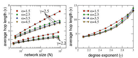
We use the model to generate scale-free networks with different values of power-law degree distribution exponent $\gamma$ and clustering strength $\alpha$, covering the observed values in a vast majority of documented complex networks Albert and Barabási (2002); Newman (2003); Dorogovtsev and Mendes (2003). We then simulate greedy routing for a large sample of paths on all generated networks, and compare the following two navigability parameters: 1) the average hop length $\tau$ from source to destination of successful greedy-routing paths, and 2) the success ratio $p_{s}$, defined as the percentage of successful paths. Unsuccessful paths are paths that get stuck at nodes without neighbours closer to the destination in the hidden space than themselves. These nodes usually have small degrees. See Appendix B for simulation details.

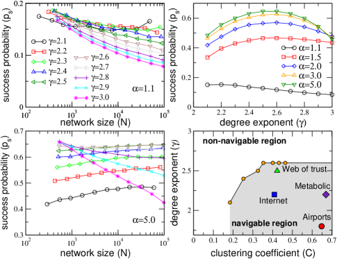
Fig. 2 shows the impact of the network’s degree distribution and clustering on the average length $\tau$ of greedy routing paths. We observe a straightforward dependency: paths are shorter for smaller exponents $\gamma$ and stronger clustering (larger $\alpha$’s). The dependency of the success ratio (the fraction of successful paths) $p_{s}$ on the two topology parameters $\gamma$ and $\alpha$ is more intertwined. Fig. 3 shows that the effect of one parameter, $\gamma$, on the success ratio depends on the other parameter, the level of clustering. If clustering is weak (low $\alpha$), the percentage of successful paths decays with network size $N$ regardless of the value of $\gamma$ (Fig. 3 top-left). However, with strong clustering (large $\alpha$), the percentage of successful paths increases with $N$ and attains a maximum for large networks if $\gamma\lesssim 2.6$, whereas it degrades for large networks if $\gamma>2.6$ (Fig. 3 bottom-left). Fig. 3 top-right shows this effect for networks of the same size ($N=10^{5}$) with different $\gamma$ and $\alpha$. The value of $\gamma=2.6\pm 0.1$ maximises the number of successful paths once clustering is above a threshold, $\alpha\geq 1.5$. These observations mean that for a fixed clustering strength, there is a critical value of the exponent $\gamma$ (Fig. 3 bottom-right) below which networks remain navigable as their size increases, but above which their navigability deteriorates with their size.

In summary, strong clustering improves both navigability metrics. We also find a delicate trade-off between values of $\gamma$ close to $2$ minimising path lengths, and higher values – not exceeding $\gamma\approx 2.6$ – maximising the percentage of successful paths. We explain these findings in the next section, but we note here that qualitatively, this navigable parameter region contains a majority of complex networks observed in reality Albert and Barabási (2002); Newman (2003); Dorogovtsev and Mendes (2003), as confirmed in Fig. 3 (bottom-right), where we juxtapose few paradigmatic examples of communication, social, biological, and transportation networks vs. the identified navigable region of clustering and degree distribution exponent. Interestingly, power grids, which propagate electricity rather than route information, are neither scale-free nor clustered Watts and Strogatz (1998); Amaral et al. (2000).

IV Air travel by greedy routing as an explanation

Figure 4: Greedy routing in the airport network. Top: the structure of the single greedy-routing path from Toksook Bay to Ibiza. At each intermediate airport, the next hop is the airport closest to Ibiza geographically. Sizes of symbols representing the airports are proportional to the logarithm of their degrees. The bottom left figure shows the changing distance to Ibiza (in the $x$ axis) vs. the degree of the visited airports ($y$ axis, in logarithmic scale). Bottom right: the structure of greedy-routing paths between a collection of airports in the USA USA . We include an airport pair in the collection if the distance between the airports is between $3900$ and $4100$ kilometers. The number of airport pairs in this collection is $7620$. We use colour to indicate how often paths in the collection go through an airport of a given degree located at a given geographical distance from the destination: blue/red indicates exponentially less/more visits to those airports, or more specifically, the color is the logarithm of the normalised density of visited airports.

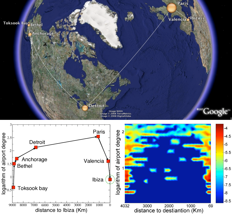
We illustrate the greedy routing function, and the structure of networks conductive to such routing, with an example of passenger air travel. Suppose we want to travel from Toksook Bay, Alaska, to Ibiza, Spain, by the public air transportation network. Nodes in this network are airports, and two airports are connected if there is at least one flight between them. We travel according to the greedy routing strategy using geography as the underlying metric space. At each airport we choose the next-hop airport geographically closest to the destination. Under these settings, our journey goes first to Bethel, then to Anchorage, to Detroit, over the Atlantic to Paris, then to Valencia and finally to Ibiza, see Fig. 4. The sequence and sizes of airport hops reveal the structure of our greedy-routing path. The path proceeds from a small airport to a local hub at a small distance, from there to a larger hub at a larger distance, and so on until we reach Paris. At that point, when the distance to the destination becomes sufficiently small, greedy routing leads us closer to our final destination by choosing not another hub, but a less connected neighbouring airport.

We observe that the navigation process has two, somewhat symmetric phases. The first phase is a coarse-grained search, travelling longer and longer distances per hop toward hubs, thus “zooming out” from the starting point. The second phase corresponds to a fine-grained search, “zooming in” onto the destination. The turning point between the two phases appears naturally: once we are in a hub near the destination, the probability that it is connected to a bigger hub closer to the destination sharply decreases, but at this point we do not need hubs anyway, and greedy routing directs us to smaller airports at shorter distances next to the destination.

This zoom out/zoom in mechanism works efficiently only if the coupling between the airport network topology and the underlying geography satisfies the following two conditions: the sufficient hubs condition and the sufficient clustering condition. The first condition ensures that a network has enough hub airports (high-degree nodes) to provide an increasing sequence during the zoom out phase. This condition is fulfilled by the real airport network and by other scale-free networks with small values of degree distribution exponent $\gamma$, because the smaller the $\gamma$, the larger the proportion of hubs in the network.

However, the presence of many hubs does not ensure that greedy routing will use them. Unlike humans, who can use their knowledge of airport size to selectively travel via hub airports, greedy routing uses only one constraint at each hop: minimise distance to the destination. Therefore, the network topology must satisfy the second condition, which ensures that Bethel is larger than Toksook Bay, Anchorage larger than Bethel, and so on. More generally, this condition is that the next greedy hop from a remote low-degree node likely has a higher degree, so that greedy paths typically head first toward the highly connected network core. But the network metric strength is exactly the required property: preference for connections between nodes nearby in the hidden space means that low-degree nodes are less likely to have connectivity to distant low-degree nodes; only high-degree nodes can have long-range connection that greedy routing will effectively select. The stronger this coupling between the metric space and topology (the higher $\alpha$ in Eq. (II)), the stronger the clustering in the network.

To illustrate, imagine an airport network without sufficient clustering, one where the airport closest to our destination (Ibiza) among all airports connected to our current node (Toksook Bay, Alaska) is not Bethel, which is bigger than Toksook Bay, but Nightmute, Alaska, a nearby airport of comparable size to Toksook Bay. As greedy routing first leads us to Nightmute, then to another small nearby airport, and then to another, we can no longer get to Ibiza in few hops. Worse, travelling via these numerous small airports, we could reach one with no connecting flights heading closer to Ibiza. Our greedy routing would be stuck at this airport with an unsuccessful path.

These factors explain why the most navigable topologies correspond to scale-free networks with small exponents of the degree distribution, i.e., a large number of hubs, and with strong clustering, i.e., strong coupling between the hidden geometry and the observed topology.

V The structure of greedy-routing paths

Figure 5: Probability that greedy routing travels to higher-degree nodes. More precisely, the probability $P_{up}(k,d)$ that the greedy-routing next hop after a node of degree $k$ located at distance $d$ from a destination has higher degree $k^{\prime}\geq k$ and is closer to the destination. The distance legend in the right-bottom plot applies to all the plots. The results are for the large-graph limit $N\to\infty$.

Figure 6: The structure of greedy-routing paths. We visualise the results of our simulation of greedy routing in modelled networks with different values of $\gamma$ and $\alpha$ observed in real complex networks. The hidden distance between the starting point and the destination is always approximately $10^{4}$, and the network size $N$ and number of attempted paths is always $10^{5}$ for each $(\gamma,\alpha)$ combination, but the number of successful paths and path hop-lengths vary, cf. Figs. 2,3. All paths start and end at low-degree nodes located, respectively, in the left- and right-bottom corners of the diagrams (see top left plot). For each $(\gamma,\alpha)$ we depict a single typical path in black and, as in Fig. 4, use colour to indicate how often paths included a node of a given degree located at a given distance from the destination. The simulations confirm that only when $\gamma$ is small and $\alpha$ is large does the average path structure follow the zoom-out/zoom-in pattern that characterises successful greedy routing in real networks, e.g., in the airport network in Fig. 4.

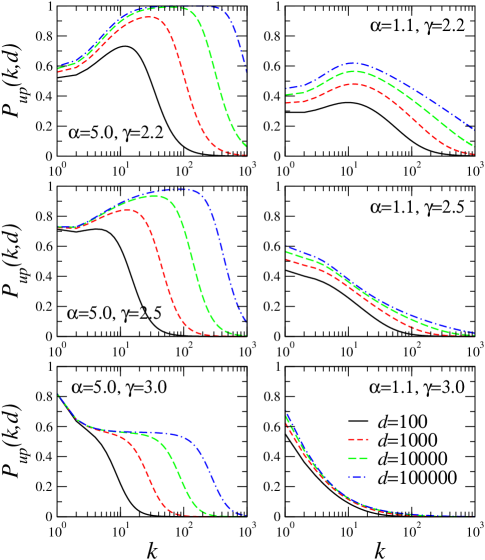
We observe the discussed zoom-out/zoom-in mechanism in analytical calculations and numerical simulations. Specifically, we calculate (in Appendix F) the probability that the next hop from a node of degree $k$ located at hidden distance $d$ from the destination has a larger degree $k^{\prime}>k$, in which case the path moves toward the high-degree network core, see Fig. 5. In the most navigable case, with small degree-distribution exponent and strong clustering, the probability of increasing the node degree along the path is high at low-degree nodes, and sharply decreases to zero after reaching a node of a critical degree value, which increases with distance $d$. This observation implies that greedy-routing paths first propagate up to higher-degree nodes in the network core and then exit the core toward low-degree destinations in the periphery. In contrast, with low clustering, paths are less likely to find higher-degree nodes regardless of the distance to the destination. This path structure violates the zoom-out/zoom-in pattern required for efficient navigation.

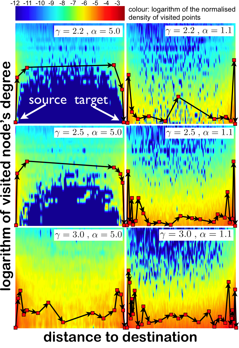
Fig. 6 shows the structure of greedy-routing paths in simulations, further confirming our analysis. We again see that for small degree-distribution exponents and strong clustering (upper left and middle left), the routing process quickly finds a way to the high-degree core, makes a few hops there, and then descends to a low-degree destination. In the other, non-navigable cases, the process can almost never get to the core of high-degree nodes. Instead, it wanders in the low-degree periphery increasing the probability of getting lost at low-degree nodes.

VI Discussion

Our main motivation for this work comes from long-standing scalability problems with the Internet routing architecture Meyer et al. (2007). To route information packets to a given destination, Internet routers must communicate to maintain a coherent view of the global Internet topology. The constantly increasing size and dynamics of the Internet thus leads to immense and quickly growing communication and information processing overhead, a major bottleneck in routing scalability Krioukov et al. (2007) causing concerns among Internet experts that the existing Internet routing architecture may not sustain even another decade Meyer et al. (2007). Discovery of the Internet’s hidden metric space would remove this bottleneck, eliminating the need for the inherently unscalable communication of topology changes. Instead routers would be able to just forward packets greedily to the destination based on hidden distances.

In a similar manner, reconstruction of hidden metric spaces underlying other real networks may prove practically useful. For example, in social or communication networks (e.g., the Web, overlay, or online social networks) hidden spaces would yield efficient strategies for searching specific individuals or content based only on local knowledge. The metric spaces hidden under some biological networks (such as neural, gene regulatory networks, signalling or even protein folding Ravasz et al. (2007) pathways) can become a powerful tool in studying the structure of information or signal flows in these networks, enabling investigation of such processes without detailed global knowledge of the network structure or organisation.

The natural question we thus face is how to proceed toward discovery of the explicit structure of hidden metric spaces underlying real networks. We do not expect spaces underlying different networks to be exactly the same. For example, the similarity spaces of Web pages Menczer (2002) and Wikipedia editors Crandall et al. (2008) likely differ. However, the main contribution of this work establishes the general mechanisms behind navigability of scale-free, strongly clustered topologies that characterise many different real networks. The next step is to find the common properties of hidden spaces that render them congruent with these mechanisms. Specifically, we are interested in what geometries of hidden spaces lead to such congruency Krioukov et al. (2008).

In general, we believe that the present and future work on hidden metric spaces and network navigability will deepen our understanding of the fundamental laws describing relationships between structure and function of complex networks.

Appendix A A model with the circle as a hidden metric space.

In our model we place all nodes on a circle by assigning them a random variable $\theta$, i.e., their polar angle, distributed uniformly in $[0,2\pi)$. The circle radius $R$ grows linearly with the total number of nodes $N$, $2\pi R=N$, in order to keep the average density of nodes on the circle fixed to $1$. We next assign to each node its expected degree $\kappa$ drawn from some distribution $\rho(\kappa)$. The connection probability between two nodes with hidden co-ordinates $(\theta,\kappa)$ and $(\theta^{\prime},\kappa^{\prime})$ takes the form

$$r(\theta,\kappa;\theta^{\prime},\kappa^{\prime})=\left(1+\frac{d(\theta,\theta^{\prime})}{\mu\kappa\kappa^{\prime}}\right)^{-\alpha},\quad\mu=\frac{(\alpha-1)}{2\langle k\rangle},$$ (2)

where $d(\theta,\theta^{\prime})$ is the geodesic distance between the two node on the circle, while $\langle k\rangle$ is the average degree. One can show that the average degree of nodes with hidden variable $\kappa$, $\bar{k}(\kappa)$, is proportional to $\kappa$.Boguñá and Pastor-Satorras (2003)   This proportionality guarantees that the shape of the node degree distribution $P(k)$ in generated networks is approximately the same as the shape of $\rho(\kappa)$. The choice of $\rho(\kappa)=(\gamma-1)\kappa_{0}^{\gamma-1}\kappa^{-\gamma}$, $\kappa>\kappa_{0}\equiv(\gamma-2)\langle k\rangle/(\gamma-1)$, $\gamma>2$, generates random networks with a power-law degree distribution of the form $P(k)\sim k^{-\gamma}$, where $\gamma$ is a model parameter that regulates the heterogeneity of the degree distribution in the network. This parameter abstracts the heterogeneity of node degrees in real networks, where degree distributions may not perfectly follow power laws, or may exhibit various forms of high-degree cut-offs M. Giot et al. (2003); Mahadevan et al. (2006). The specific effects are less important than the overall measure of heterogenity. We note that instead of a circle in our model we could use any isotropic space of any dimension Ángeles Serrano et al. (2008).

Appendix B Numerical simulations.

Our model has three independent parameters: exponent $\gamma$ of power-law degree distributions, clustering strength $\alpha$, and average degree $\langle k\rangle$. We fix the latter to $6$, which is roughly equal to the average degree of some real networks of interest Mahadevan et al. (2006); Boguñá et al. (2004a), and vary $\gamma\in[2.1,3]$ and $\alpha\in[1.1,5]$, covering their observed ranges in documented complex networks Albert and Barabási (2002); Newman (2003); Dorogovtsev and Mendes (2003). For each $(\gamma,\alpha)$ pair, we produce networks of different sizes $N\in[10^{3},10^{5}]$ generating, for each $(\gamma,\alpha,N)$, a number of different network instances—from $40$ for large $N$ to $4000$ for small $N$. In each network instance $G$, we randomly select $10^{6}$ source-destination pairs $(a,b)$ and execute the greedy-routing process for them starting at $a$ and selecting, at each hop $h$, the next hop as the $h$’s neighbour in $G$ closest to $b$ in the circle. If for a given $(a,b)$, this process visits the same node twice, then the corresponding path leads to a loop and is unsuccessful. We then average the measured values of path hop lengths $\tau$ and percentage of successful paths $p_{s}$ across all pairs $(a,b)$ and networks $G$ for the same $(\gamma,\alpha,N)$. Note that we are not concerned with the absolute values of the success ratio $p_{s}$. Instead we use it as a measure of navigability to compare networks with different $(\gamma,\alpha,N)$. For this purpose we could use the success ratio of any (improved) modification of standard greedy routing.

Appendix C Shortest path vs. shortest time.

All results derived in the present paper are about finding short paths across a network topology. The total physical time from source to destination is implicitly assumed to be proportional to the number of hops. In real transportation systems, e.g. the Internet or the airport network, the finite capacity of nodes implies that the end-to-end path latency may be longer when intermediate nodes are congested. While our results most cleanly apply to uncongested systems, there are obvious modifications, such as choosing the second or third nearest rather than the nearest neighbor, that could still find nearly shortest paths while reducing and balancing load on the system.

Appendix D The model vs. real networks: the Autonomous System level map of the Internet and the US Airport Network

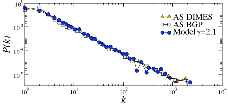
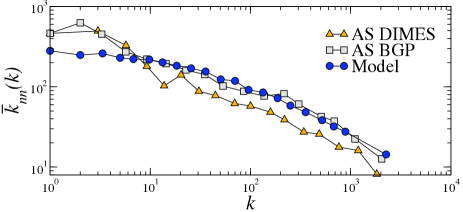
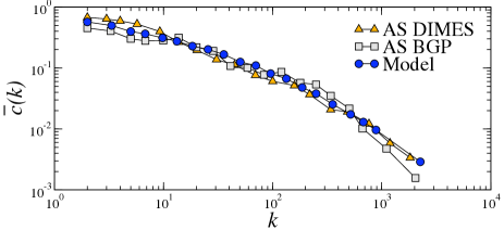
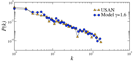
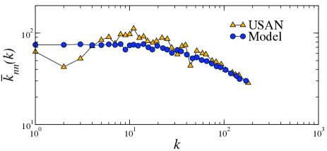
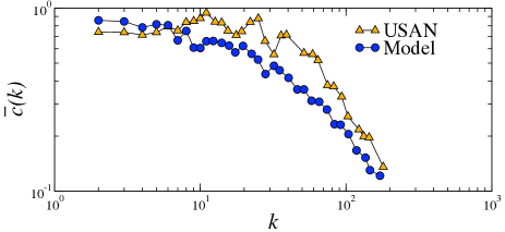
The model we use in this work is not meant to reproduce any particular system but to generate a set of general properties, like heterogeneous degree distributions, high clustering, and a metric structure lying underneath. Yet, despite its simplistic assumptions, the model generates graphs that are surprisingly close to some real networks of interest, in particular the Internet at the Autonomous System level (AS) Mahadevan et al. (2006); Shavitt and Shir (2005) and the network of airline connections among airports within the United States during 2006 (USAN) USA . In the case of the Internet, we use two different data sets, the Internet as viewed by the Border Gateway Protocol (BGP) Mahadevan et al. (2006) and the DIMES project Shavitt and Shir (2005). The BGP (DIMES) network has a size of $N\sim 17446$ ($N=19499$) ASs, average degree $\langle k\rangle=4.7$ ($\langle k\rangle=5$), and average clustering $C=0.41$ ($C=0.6$). The US Airport Network is composed of US airports connected by regular flights (with more than 1000 passengers per year) during the year $2006$. This results in a network of $N=599$ airports, average degree $\langle k\rangle\sim 10.8$ and average clustering coefficient $C=0.72$.

Figs. 7 and 8 show a comparison of the basic topological properties of these networks with graphs generated with the model. In the case of the AS map, we use a truncated power law distribution $\rho(\kappa)\sim\kappa^{-\gamma}$, $\kappa<\kappa_{c}$ with exponent $\gamma=2.1$ and $\kappa_{c}$ such that the maximum degree of the network is $k_{c}=2400$. For the USAN, we use $\gamma=1.6$ and a maximum degree $k_{c}=180$, as observed in the real network. As it can be appreciated in both figures, the matching of the model with the empirical data is surprisingly good except for very low degree vertices. This is particularly interesting since we are not enforcing any mechanism to reproduce higher order statistics like the average nearest neighbours degree $\bar{k}_{nn}(k)$ or the degree-dependent clustering coefficient $\bar{c}(k)$. This can be understood as a consequence of the high heterogeneity of the degree distribution that introduces structural constraints in the network Park and Newman (2003); Boguñá et al. (2004b).

The airport network differs in several ways from our modelled networks: the distribution of airports in the geographic space is far from uniform; the airport degree distribution does not perfectly follow a power law; and it exhibits a sharp high-degree cut-off. However, the structure of greedy paths is surprisingly similar to that in our modelled networks in Fig. 6. The success ratio $p_{s}\approx 0.64$ and average length of successful paths $\tau\approx 2.1$ are also similar to those in our modelled networks of the corresponding size, clustering, and degree distribution exponent. These similarities indicate that the network navigability characteristics depend on clustering and heterogeneity of the airport degree distribution, and less so on how perfectly it follows a power law.

Appendix E Hierarchical organization of modeled networks

The routing process in our framework resembles guided searching for a specific object in a complex collection of objects. Perhaps the simplest and most general way to make a complex collection of heterogenous objects searchable is to classify them in a hierarchical fashion. By “hierarchical,” we mean that the whole collection is split into categories (i.e., sets), sub-categories, sub-sub-categories, and so on. Relationships between categories form (almost) a tree, whose leaves are individual objects in the collection Watts et al. (2002); Girvan and Newman (2002); Clauset et al. (2008); Krioukov et al. (2008). Finding an object reduces to the simpler task of navigating this tree.

Figure 7: Degree distribution $P(k)$, average nearest neighbours’ degree $\bar{k}_{nn}(k)$, and degree-dependent clustering coefficient $\bar{c}(k)$ generated by our model with $\gamma=2.1$ and $\alpha=2$ compared to the same metrics for the real Internet map as seen by BGP data and the DIMES project.

Figure 8: Degree distribution $P(k)$, average nearest neighbours’ degree $\bar{k}_{nn}(k)$, and degree-dependent clustering coefficient $\bar{c}(k)$ generated by our model with $\gamma=1.6$, $\alpha=5$ and a cut-off at $k_{c}=180$ compared to the same metrics for the real US airport network.

Figure 9: $k$-core decompositions of real and modeled networks. The first two rows show LaNet-vi Alvarez-Hamelin et al. (2006) network visualizations. All nodes are color-coded based on their coreness (right legends) and size-coded based on their degrees (left legends). Higher-coreness nodes are closer to circle centers. The third row shows the $k$-core spectrum, i.e., the distribution ${\cal S}(k)$ of sizes of node sets with coreness $k$. The first column depicts two real networks: the AS-level Internet as seen by the Border Gateway Protocol (BGP) in Mahadevan et al. (2006) and the Pretty Good Privacy (PGP) social network from Boguñá et al. (2004a). The rest of the columns show modeled networks for different values of power-law exponent $\gamma$ in cases with weak ($\alpha=1.1$) and strong ($\alpha=5.0$) clustering. The network size $N$ for all real and modeled cases is approximately $10^{4}$. Similarity between real networks and modeled networks with low $\gamma$ and high $\alpha$ is remarkable.

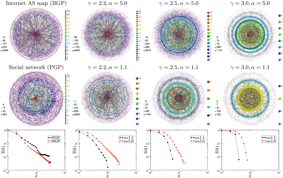
$k$-core decomposition Bollobás (1998); Dorogovtsev et al. (2006) is possibly the most suitable generic tool to expose hierarchy within our modeled networks. The $k$-core of a network is its maximal subgraph such that all the nodes in the subgraph have $k$ or more connections to other nodes in the subgraph. A node’s coreness is the maximum $k$ such that the $k$-core contains the node but the $k+1$-core does not. The $k$-core structure of a network is a form of hierarchy since a $k+1$-core is a subset of a $k$-core. One can estimate the quality of this hierarchy using properties of the $k$-core spectrum, i.e., the distribution of $k$-core sizes. If the maximum node coreness is large and if there is a rich collection of comparably-sized $k$-cores with a wide spectrum of $k$’s, then this hierarchy is deep and well-developed, making it potentially more navigable. It is poor, non-navigable otherwise.

In Fig. 9 we feed real and modeled networks to the Large Network visualization tool (LaNet-vi) Alvarez-Hamelin et al. (2006) which utilizes node coreness to visualize the network. Fig. 9 shows that networks with stronger clustering and smaller exponents of degree distribution possess stronger $k$-core hierarchies. These hierarchies are directly related to how networks are constructed in our model, since nodes with higher $\kappa$ and, consequently, higher degrees have generally higher coreness, as we can partially see in Fig. 9.

Appendix F The one-hop propagator of greedy routing

To derive the greedy-routing propagator in this appendix, we adopt a slightly more general formalism than in the main text. Specifically, we assume that nodes live in a generic metric space $\cal H$ and, at the same time, have intrinsic attributes unrelated to $\cal H$. Contrary to normed spaces or Riemannian manifolds, generic metric spaces do not admit any coordinates, but we still use the coordinate-based notations here to simplify the exposition below, and denote by ${\bf x}$ nodes’ coordinates in $\cal H$ and by $\omega$ all their other, non-geometric attributes, such as their expected degree $\kappa$. In other words, hidden variables ${\bf x}$ and $\omega$ in this general formalism represent some collections of nodes’ geometric and non-geometric hidden attributes, not just a pair of scalar quantities. Therefore, integrations over ${\bf x}$ and $\omega$ in what follows stand merely to denote an appropriate form of summation in each concrete case.

As in the main text, we assume that ${\bf x}$ and $\omega$ are independent random variables so that the probability density to find a node with hidden variables $({\bf x},\omega)$ is

$$\rho({\bf x},\omega)=\delta({\bf x})\rho(\omega)/N,$$ (3)

where $\rho(\omega)$ is the probability density of the $\omega$ variables and $\delta({\bf x})$ is the concentration of nodes in ${\cal H}$. The total number of nodes is

$$N=\int_{\cal H}\delta({\bf x})d{\bf x},$$ (4)

and the connection probability between two nodes is an integrable decreasing function of the hidden distance between them,

$$r({\bf x},\omega;{\bf x}^{\prime},\omega^{\prime})=r[d({\bf x},{\bf x}^{\prime})/d_{c}(\omega,\omega^{\prime})],$$ (5)

where $d_{c}(\omega,\omega^{\prime})$ a characteristic distance scale that depends on $\omega$ and $\omega^{\prime}$.

We define the one-step propagator of greedy routing as the probability $G({\bf x}^{\prime},\omega^{\prime}|{\bf x},\omega;{\bf x}_{t})$ that the next hop after a node with hidden variables $({\bf x},\omega)$ is a node with hidden variables $({\bf x}^{\prime},\omega^{\prime})$, given that the final destination is located at ${\bf x}_{t}$.

To further simplify the notations below, we label the set of variables $({\bf x},\omega)$ as a generic hidden variable $h$ and undo this notation change at the end of the calculations according to the following rules:

$$\begin{array}[]{rcl}({\bf x},\omega)&\longrightarrow&h\\ \rho({\bf x},\omega)&\longrightarrow&\rho(h)\\ d{\bf x}d\omega&\longrightarrow&dh\\ r({\bf x},\omega;{\bf x}^{\prime},\omega^{\prime})&\longrightarrow&r(h,h^{\prime}).\end{array}$$ (6)

We begin the propagator derivation assuming that a particular network instance has a configuration given by $\{h,h_{t},h_{1},\cdots,h_{N-2}\}\equiv\{h,h_{t};\{h_{j}\}\}$ with $j=1,\cdots,N-2$, where $h$ and $h_{t}$ denote the hidden variables of the current hop and the destination, respectively. In this particular network configuration, the probability that the current node’s next hop is a particular node $i$ with hidden variable $h_{i}$ is the probability that the current node is connected to $i$ but disconnected to all nodes that are closer to the destination than $i$,

$$\mbox{Prob}(i|h,h_{t};\{h_{j}\})=r(h,h_{i})\displaystyle{\prod_{j(\neq i)=1}^{N-2}}\left[1-r(h,h_{j})\right]^{\Theta\left[d(h_{i},h_{t})-d(h_{j},h_{t})\right]},$$ (7)

where $\Theta(\cdot)$ is the Heaviside step function. Taking the average over all possible configurations $\{h_{1},\cdots,h_{i-1},h_{i+1},\cdots,h_{N-2}\}$ excluding node $i$, we obtain

$$\mbox{Prob}(i|h,h_{t};h_{i})=r(h,h_{i})\left(1-\frac{1}{N-3}\bar{k}(h|h_{i},h_{t})\right)^{N-3},$$ (8)

where

$$\bar{k}(h|h_{i},h_{t})=(N-3)\int_{d(h_{i},h_{t})<d(h^{\prime},h_{t})}\rho(h^{\prime})r(h,h^{\prime})dh^{\prime}$$ (9)

is the average number of connections between the current node and nodes closer to the destination than node $i$, excluding $i$ and $t$.

The probability that the next hop has hidden variable $h^{\prime}$, regardless of its label, i.e., index $i$, is

$$\mbox{Prob}(h^{\prime}|h,h_{t})=\sum_{i=1}^{N-2}\rho(h^{\prime})\mbox{Prob}(i|h,h_{t};h^{\prime}).$$ (10)

In the case of sparse networks, $\bar{k}(h|h^{\prime},h_{t})$ is a finite quantity. Taking the limit of large $N$, the above expression simplifies to

$$\mbox{Prob}(h^{\prime}|h,h_{t})=N\rho(h^{\prime})r(h,h^{\prime})e^{-\bar{k}(h|h^{\prime},h_{t})}.$$ (11)

Yet, this equation is not a properly normalized probability density function for the variable $h^{\prime}$ since node $h$ can have degree zero with some probability. If we consider only nodes with degrees greater than zero, then the normalization factor is given by $1-e^{-\bar{k}(h)}$. Therefore, the properly normalized propagator is finally

$$G(h^{\prime}|h,h_{t})=\displaystyle{\frac{N\rho(h^{\prime})r(h,h^{\prime})e^{-\bar{k}(h|h^{\prime},h_{t})}}{1-e^{-\bar{k}(h)}}}.$$ (12)

We now undo the notation change and express this propagator in terms of our mixed coordinates:

$$G({\bf x}^{\prime},\omega^{\prime}|{\bf x},\omega;{\bf x}_{t})=\frac{\delta({\bf x}^{\prime})\rho(\omega^{\prime})}{1-e^{-\bar{k}({\bf x},\omega)}}r\left[\frac{d({\bf x},{\bf x}^{\prime})}{d_{c}(\omega,\omega^{\prime})}\right]e^{-\bar{k}({\bf x},\omega|{\bf x}^{\prime},{\bf x}_{t})},$$ (13)

with

$$\bar{k}({\bf x},\omega|{\bf x}^{\prime},{\bf x}_{t})=\int_{d({\bf x}^{\prime},{\bf x}_{t})>d({\bf y},{\bf x}_{t})}d{\bf y}\int d\omega^{\prime}\delta({\bf y})\rho(\omega^{\prime})r\left[\frac{d({\bf x},{\bf y})}{d_{c}(\omega,\omega^{\prime})}\right].$$ (14)

In the particular case of the $\mathbb{S}^{1}$ model, we can express this propagator in terms of relative hidden distances instead of absolute coordinates. Namely, $G(d^{\prime},\omega^{\prime}|d,\omega)$ is the probability that an $\omega$-labeled node, e.g., a node with expected degree $\kappa=\omega$, at hidden distance $d$ from the destination has as the next hop an $\omega^{\prime}$-labeled node at hidden distance $d^{\prime}$ from the destination. After tedious calculations, the resulting expression reads:

$$\footnotesize G(d^{\prime},\omega^{\prime}|d,\omega)=\left\{\begin{array}[]{ll}\frac{(\gamma-1)}{\omega^{\prime\gamma}}\left[\frac{1}{(1+\frac{d-d^{\prime}}{\mu\omega\omega^{\prime}})^{\alpha}}+\frac{1}{(1+\frac{d+d^{\prime}}{\mu\omega\omega^{\prime}})^{\alpha}}\right]\mbox{exp}\left\{\frac{(1-\gamma)\mu\omega}{\alpha-1}\left[{\cal B}(\frac{d-d^{\prime}}{\mu\omega},\gamma-2,2-\alpha)-{\cal B}(\frac{d+d^{\prime}}{\mu\omega},\gamma-2,2-\alpha)\right]\right\}&;d^{\prime}\leq d\\[14.22636pt] \frac{(\gamma-1)}{\omega^{\prime\gamma}}\left[\frac{1}{(1+\frac{d^{\prime}-d}{\mu\omega\omega^{\prime}})^{\alpha}}+\frac{1}{(1+\frac{d+d^{\prime}}{\mu\omega\omega^{\prime}})^{\alpha}}\right]\mbox{exp}\left\{\frac{(1-\gamma)\mu\omega}{\alpha-1}\left[\frac{2}{\gamma-2}-{\cal B}(\frac{d^{\prime}-d}{\mu\omega},\gamma-2,2-\alpha)-{\cal B}(\frac{d+d^{\prime}}{\mu\omega},\gamma-2,2-\alpha)\right]\right\}&;d^{\prime}>d\end{array}\right.,$$ (15)

where we have defined function

$${\cal B}(z,a,b)\equiv z^{-a}\int_{0}^{z}t^{a-1}(1+t)^{b-1}dt,$$ (16)

which is somewhat similar to the incomplete beta function $B(z,a,b)=\int_{0}^{z}t^{a-1}(1-t)^{b-1}dt$.

Figure 10: Probability $P_{up}(\omega/d^{1/2},d)$.

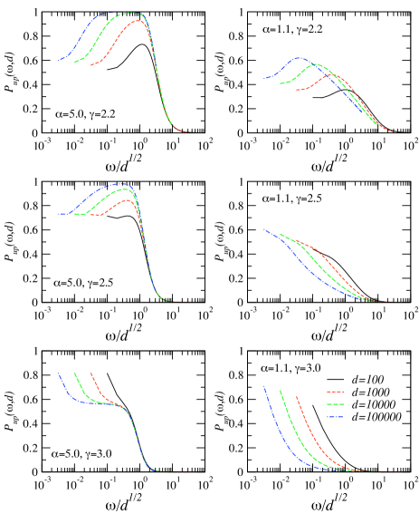
One of the informative quantities elucidating the structure of greedy-routing paths is the probability $P_{up}(\omega,d)$ that the next hop after an $\omega$-labeled node at distance $d$ from the destination has a higher value of $\omega$. The greedy-routing propagator defines this probability as

$$P_{up}(\omega,d)=\int_{\omega^{\prime}\geq\omega}d\omega^{\prime}\int_{d^{\prime}<d}dd^{\prime}G(d^{\prime},\omega^{\prime}|d,\omega),$$ (17)

and we show $P_{up}(\omega/d^{1/2},d)$ in Fig. 10. We see that the proper scaling of $\omega_{c}\sim d^{1/2}$, where $\omega_{c}$ is the critical value of $\omega$ above which $P_{up}(\omega,d)$ quickly drops to zero, is present only when clustering is strong. Furthermore, $P_{up}(\omega,d)$ is an increasing function of $\omega$ for small $\omega$’s only when the degree distribution exponent $\gamma$ is close to $2$. A combination of these two effects guarantees that the layout of greedy routes properly adapts to increasing distances or graph sizes, thus making networks with strong clustering and $\gamma$’s greater than but close to $2$ navigable.

References

- Albert and Barabási (2002) R. Albert and A.-L. Barabási, Rev. Mod. Phys. 74, 47 (2002).
- Newman (2003) M. E. J. Newman, SIAM Rev 45, 167 (2003).
- Dorogovtsev and Mendes (2003) S. N. Dorogovtsev and J. F. F. Mendes, Evolution of networks: From biological nets to the Internet and WWW (Oxford University Press, Oxford, 2003).
- Boccaletti et al. (2006) S. Boccaletti, V. Latora, Y. Moreno, M. Chavez, and D.-U. Hwang, Phys. Rep. 424, 175 (2006).
- Castells (1996) M. Castells, The rise of the network society (Blackwell Publishing, Oxford, 1996).
- Pastor-Satorras and Vespignani (2004) R. Pastor-Satorras and A. Vespignani, Evolution and Structure of the Internet. A Statistical Physics Approach (Cambridge University Press, Cambridge, 2004).
- Watts et al. (2002) D. J. Watts, P. S. Dodds, and M. E. J. Newman, Science 296, 1302 (2002).
- Girvan and Newman (2002) M. Girvan and M. E. J. Newman, Proc. Nat. Acad. Sci. USA 99, 7821 (2002).
- Menczer (2002) F. Menczer, Proc. Nat. Acad. Sci. USA 99, 14014 (2002).
- Leicht et al. (2006) E. A. Leicht, P. Holme, and M. E. J. Newman, Phys Rev E 73, 026120 (2006).
- Crandall et al. (2008) D. Crandall, D. Cosley, D. Huttenlocher, J. Kleinberg, and S. Suri, in Proceedings of the ACM International Conference on Knowledge Discovery and Data Mining (ACM, 2008).
- Clauset et al. (2008) A. Clauset, C. Moore, and M. E. J. Newman, Nature 453, 98 (2008).
- Ángeles Serrano et al. (2008) M. Ángeles Serrano, D. Krioukov, and M. Boguñá, Phys Rev Lett 100, 078701 (2008).
- Travers and Milgram (1969) J. Travers and S. Milgram, Sociometry 32, 425 (1969).
- Watts and Strogatz (1998) D. J. Watts and S. H. Strogatz, Nature 393, 440 (1998).
- Kleinberg (2000a) J. Kleinberg, Nature 406, 845 (2000a).
- Kleinberg (2000b) J. Kleinberg, in STOC ’00: Proceedings of the thirty-second annual ACM symposium on Theory of computing (ACM, New York, NY, USA, 2000b), pp. 163–170, ISBN 1-58113-184-4.
- Kleinberg (2001) J. M. Kleinberg, in NIPS, edited by T. G. Dietterich, S. Becker, and Z. Ghahramani (MIT Press, 2001), pp. 431–438.
- Manku et al. (2004) G. S. Manku, M. Naor, and U. Wieder, in Proceedings of the 36th ACM Symposium on Theory of Computing (STOC) (ACM, 2004), pp. 54–63.
- Martel (2004) C. Martel, in 23rd ACM Symp. on Principles of Distributed Computing (PODC) (ACM Press, 2004), pp. 179–188.
- Nguyen and Martel (2005) V. Nguyen and C. Martel, in SODA ’05: Proceedings of the sixteenth annual ACM-SIAM symposium on Discrete algorithms (Society for Industrial and Applied Mathematics, Philadelphia, PA, USA, 2005), pp. 311–320, ISBN 0-89871-585-7.
- Nguyen and Martel (2008) V. Nguyen and C. Martel, in Proceedings of the Fourth Workshop on Analytic Algorithmics and Combinatorics (SIAM, 2008), pp. 213–227.
- Simsek and Jensen (2005) Ö. Simsek and D. Jensen, in IJCAI, edited by L. P. Kaelbling and A. Saffiotti (Professional Book Center, 2005), pp. 304–310, ISBN 0938075934.
- Lebhar and Schabanel (2004) E. Lebhar and N. Schabanel, in ICALP, edited by J. Díaz, J. Karhumäki, A. Lepistö, and D. Sannella (Springer, 2004), vol. 3142 of Lecture Notes in Computer Science, pp. 894–905, ISBN 3-540-22849-7.
- Fraigniaud (2005) P. Fraigniaud, in ESA, edited by G. S. Brodal and S. Leonardi (Springer, 2005), vol. 3669 of Lecture Notes in Computer Science, pp. 791–802, ISBN 3-540-29118-0.
- Fraigniaud et al. (2006) P. Fraigniaud, C. Gavoille, and C. Paul, Distrib Comput 18, 279 (2006).
- Fraigniaud et al. (2007) P. Fraigniaud, C. Gavoille, A. Kosowski, E. Lebhar, and Z. Lotker, in SPAA, edited by P. B. Gibbons and C. Scheideler (ACM, 2007), pp. 1–7, ISBN 978-1-59593-667-7.
- Fraigniaud and Gavoille (2008) P. Fraigniaud and C. Gavoille, in SPAA, edited by F. M. auf der Heide and N. Shavit (ACM, 2008), pp. 62–69, ISBN 978-1-59593-973-9.
- Chaintreau et al. (2008) A. Chaintreau, P. Fraigniaud, and E. Lebhar, in ICALP (1), edited by L. Aceto, I. Damgård, L. A. Goldberg, M. M. Halldórsson, A. Ingólfsdóttir, and I. Walukiewicz (Springer, 2008), vol. 5125 of Lecture Notes in Computer Science, pp. 133–144, ISBN 978-3-540-70574-1.
- Kleinberg (2006) J. Kleinberg, Proc. Int. Congr. Math. (ICM) 3, 1019 (2006).
- Mahadevan et al. (2006) P. Mahadevan, D. Krioukov, M. Fomenkov, B. Huffaker, X. Dimitropoulos, kc claffy, and A. Vahdat, Comput Commun Rev 36, 17 (2006).
- Boguñá et al. (2004a) M. Boguñá, R. Pastor-Satorras, A. Díaz-Guilera, and A. Arenas, Phys Rev E 70, 056122 (2004a).
- Jeong et al. (2000) H. Jeong, B. Tombor, R. Albert, Z. N. Oltvai, and A.-L. Barabási, Nature 407, 651 (2000).
- Barrat et al. (2004) A. Barrat, M. Barthélemy, R. Pastor-Satorras, and A. Vespignani, Proc. Natl. Acad. Sci. USA 101, 3747 (2004).
- Amaral et al. (2000) L. A. N. Amaral, A. Scala, M. Barthélemy, and H. E. Stanley, Proc. Nat. Acad. Sci. 97, 11149 (2000).
- (36) Data available at http://www.transtats.bts.gov/.
- Meyer et al. (2007) D. Meyer, L. Zhang, and K. Fall, eds., RFC4984 (The Internet Architecture Board, 2007).
- Krioukov et al. (2007) D. Krioukov, kc claffy, K. Fall, and A. Brady, Comput Commun Rev 37, 41 (2007).
- Ravasz et al. (2007) E. Ravasz, S. Gnanakaran, and Z. Toroczkai, Network structure of protein folding pathways (2007), arXiv:0705.0912.
- Krioukov et al. (2008) D. Krioukov, F. Papadopoulos, M. Boguñá, and A. Vahdat, Efficient navigation in scale-free networks embedded in hyperbolic metric spaces (2008), arXiv:0805.1266.
- Boguñá and Pastor-Satorras (2003) M. Boguñá and R. Pastor-Satorras, Phys Rev E 68, 036112 (2003).
- M. Giot et al. (2003) M. Giot et al., Science 302, 1727 (2003).
- Shavitt and Shir (2005) Y. Shavitt and E. Shir, Comput Commun Rev 35 (2005).
- Park and Newman (2003) J. Park and M. E. J. Newman, Phys. Rev. E 68, 026112 (2003).
- Boguñá et al. (2004b) M. Boguñá, R. Pastor-Satorras, and A. Vespignani, European Physical Journal B 38, 205 (2004b).
- Alvarez-Hamelin et al. (2006) J. I. Alvarez-Hamelin, L. Dall’Asta, A. Barrat, and A. Vespignani, in Advances in Neural Information Processing Systems 18, edited by Y. Weiss, B. Schölkopf, and J. Platt (MIT Press, Cambridge, MA, 2006), pp. 41–50.
- Bollobás (1998) B. Bollobás, Modern Graph Theory (Springer-Verlag, New York, 1998).
- Dorogovtsev et al. (2006) S. N. Dorogovtsev, A. V. Goltsev, and J. F. F. Mendes, Phys Rev Lett 96, 040601 (2006).