Improving the consensus performance via predictive mechanisms

Abstract

Considering some predictive mechanisms, we show that ultrafast average-consensus can be achieved in networks of interconnected agents. More specifically, by predicting the dynamics of the network several steps ahead and using this information in the design of the consensus protocol of each agent, drastic improvements can be achieved in terms of the speed of consensus convergence, without changing the topology of the network. Moreover, using these predictive mechanisms, the range of sampling periods leading to consensus convergence is greatly expanded compared with the routine consensus protocol. This study provides a mathematical basis for the idea that some predictive mechanisms exist in widely-spread biological swarms, flocks, and networks. From the industrial engineering point of view, inclusion of an efficient predictive mechanism allows for a significant increase in the speed of consensus convergence and also a reduction of the communication energy required to achieve a predefined consensus performance.

I Introduction

Over the last decade, scientists have been looking for some common, possibly universal, features of the collective behaviors of animals ma07 , bacteria bud95 , cells yo04 , molecular motors as94 , as well as driven granular objects vi95 . The collective motion of a group of autonomous agents (or particles) is currently a subject of intensive research that has potential applications in biology, physics and engineering. One of the most remarkable characteristics of complex dynamical systems such as flocks of birds, schools of fish, or swarms of locusts, is the emergence of a state of collective orders in which the agents move in the same direction, i.e. an ordered state vi95 ; gr04 ; al07 . This ordered state seeking problem can be further generalized to a consensus problem sa04 ; re07 , where a group of self-propelled agents agree upon certain quantities of interest such as attitude, position, temperature, voltage, etc. Furthermore, solving consensus problems using distributed computational methods has direct implications on sensor network data fusion, load balancing, swarms/flocks, unmanned air vehicles (UAVs), attitude alignment of satellite clusters, congestion control of communication networks, multi-agent formation control, and so on ak02 ; og04 ; ar02 .

Among the most important early works on consensus problems, Fiedler fi73 showed that the second smallest eigenvalue $\lambda_{2}$, namely the algebraic connectivity, of the Laplacian matrix $L$ associated with the graph defining the network topology is directly related to the consensus speed of the network. It was also shown that a network with high algebraic connectivity is robust to both node-failures and edge-failures. In sa04 , Olfati-Saber and Murray analyzed consensus problems in networks of agents with continuous-time dynamics (basically integrators), switching topology and time-delays, and proved that decreasing the largest eigenvalue $\lambda_{N}$ of the Laplacian matrix $L$ improves the consensus robustness of the network to time-delays. Consequently, the condition number $\lambda_{N}/\lambda_{2}$ provides a measure of the consensus performance of the considered network in the sense that the smaller its value, the better the consensus performance (consensus speed and robustness to time-delays). Moreover, in sa04 , the authors also provided a feasible range of sampling rates leading to consensus in the case of discrete-time dynamic networks. In this way, the theoretical foundations of general consensus problems were established. To improve the speed of convergence towards consensus, they further proposed a method based on the addition of a few long links to a regular lattice, thus transforming it into a small-world network sa05 ; st01 . In xi04 , Xiao and Boyd transformed the fastest distributed linear averaging problem into a convex optimization problem by considering a particular per-step convergence optimization index. Additionally, they proved that, when the network topology is symmetric, the problem of finding the fastest converging linear iteration can be cast as a semidefinite programming problem, and thus can be efficiently and globally solved. In ya06 , consensus problems in a heterogeneous influence network were investigated by Yang at al. and it was shown that, by decreasing the scaling exponent in the associated power-law distribution, the ability of the network to reach direction consensus among its agents is significantly enhanced due to the leading roles played by a few hub agents.

In summary, most of the previous works achieved performance improvements, such as increasing the consensus speed, improving the robustness to nodes and edges failures, or improving the ability to deal with time-delays, solely based on the currently available information flows on the network. In these works, the computing abilities of an agent of the network is fairly limited: the agent can only observe the current behavior (state) of its neighbors and update its state according to this observation. However, in natural bio-groups, individuals generally possess some higher level of predictive computing capabilities that they use for updating their state. Experiments revealing the use of prediction mechanisms by individuals of a network have been described in the literature previously. In particular, as early as 1959, Woods wo59 designed some bee swarms experiments and provided evidences for the existence of certain predictive mechanism in bee swarms formation. In 1995, Montague et al. proposed simple hebbian learning rules to explain the predictive mechanisms used by bees when foraging in uncertain environments mo95 . Apart from the investigation of the predictive mechanisms used during swarming and foraging, several researchers focused on the predictive functions of the optical and acoustical apparatuses of individuals inside bio-groups, especially the retina and cortex go03 ; su06 ; me07 . Based on intensive experiments on the bio-eyesight systems, it was found that, when an individual observer prepared to eye-follow a displacement of the visual stimulus, the visual form of adaptation was transferred from the current fixation to the future gaze position. These reported investigations support the conjecture of the existence of some predictive mechanisms inside many bio-groups.

Figure 1: (Color online) Illustration of the predictive nature of flocks, swarms and networks.

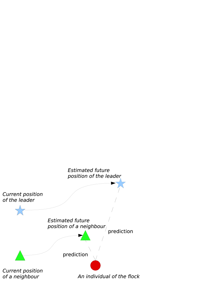
In this paper, we show that, by introducing a predictive mechanism, it is possible to either significantly enhance the consensus speed obtainable under the constraint of a fixed amount of communication energy or to decrease the communication energy required to ensure a prescribed consensus speed. This observation allows us to infer that prediction mechanisms may exist universally in many natural bio-groups. A general physical picture illustrating this paradigm is given in Fig. 1, which is interpreted as follows: in widely-spread natural bio-groups composed of animals, bacteria, cells, etc., the next-step behavioral decision of each individual/particle/agent is not only based on the current available state information (position, velocity, etc.) of the other (neighboring) agents inside the group, but is also based on their predicted future states. More precisely, bearing in mind a few past states of its leader and neighbors, an agent can estimate their future states several steps ahead and then make a decision on its own action. Estimation of these future states by each agent can eliminate the requirement of intensive communication among the agents so that the overall communication energy of the group can be reduced effectively.

From an industrial application point of view, the phenomena and mechanisms reported in this paper may be applicable in some relevant prevailing engineering areas such as autonomous robot formations, sensor networks and UAVs ak02 ; og04 ; ar02 . Each agent in such a group typically has limited power to send messages, and thus a larger sampling period is generally desirable to save communication energy. Since using a predictive mechanism can sharply expand the range of feasible sampling periods, it should be useful for industrial applications where overall communication energy is limited.

The rest of this paper is organized as follows. In Section II, the two main problems addressed in this paper are formulated. In Section III, the all-to-all link model predictive control (MPC) average-consensus protocol is presented together with its convergence analysis and some statistical simulation results. In Section IV, the MPC consensus protocol is generalized to partial link networks. Additionally, conditions that guarantee asymptotic convergence of the proposed protocol are provided, and simulation results showing its main characteristics and advantages are presented. Finally, conclusions are drawn in Section V.

II Problem description

In order to discuss and illustrate the role of prediction mechanisms in networks of interconnected agents, we consider one of the simplest type of networks, i.e. networks of linearly interconnected integrators. The interconnection structure of such networks can typically be represented by a directed graph (called digraph for short). In this representation of the network, the $N$ nodes of the digraph represent the $N$ agents of the network and a weighted edge $a_{ij}$ from node $i$ to node $j$ indicates the existence of a communication link from agent $i$ to agent $j$ in the network. The digraph is denoted by $G=(\mathcal{V},\mathcal{E},A)$, where $\mathcal{V}=\left\{v_{1},\ldots,v_{N}\right\}$ is the set of nodes, $\mathcal{E}\subset\mathcal{V}\times\mathcal{V}$ is the set of edges, and $A$ is the associated weighted adjacency matrix, i.e. $A=\left\{a_{ij}\right\}_{i,j=1,\ldots,N}\in\mathbb{R}^{N\times N}$, with nonnegative elements $a_{ij}$ which are zero when there is no communication link from $i$ to $j$. Furthermore, we assume that there is no self-cycle, i.e. $a_{ii}=0$, $\forall i=1,\ldots,N$.

Let $x_{i}(t)\in\mathbb{R}$ denote the state of node $i$, which might represent physical quantities such as attitude, position, temperature, voltage, etc. To obtain a full representation of the dynamic network under consideration, we refer to it as $G_{x}=(G,x)$ where $x\in\mathbb{R}^{N}$ denotes the network state and $G$ its topology (or information flow). Generally, we say that the nodes of a network have reached consensus if and only if $x_{i}=x_{j}$ for all $i,j\in\mathcal{V}$. Whenever the nodes of a network are all in agreement, their common value is called the group decision value. If the group decision value is $\overline{x}(0)\triangleq 1/N(\sum_{i=1}^{N}x_{i}(0))$, the network is said to have reached the average-consensus. In the rest of the paper, for brevity, we denote average-consensus by consensus.

Agents with continuous-time models are typically described by the integrator dynamics

$$\dot{x}_{i}(t)=u_{i}(t),$$ (1)

while agents with discrete-time models are described by the difference dynamics

$$x_{i}(k+1)=x_{i}(k)+\epsilon u_{i}(k),$$ (2)

where $\epsilon$ denotes the sampling period or step-size. Average-consensus is typically asymptotically reached using the routine consensus protocol

$$u_{i}(t)=-\sum_{j=1}^{N}a_{ij}\Delta x_{i,j}(t),~{}~{}i,j=1,\ldots,N,$$ (3)

where $\Delta x_{i,j}(t)\triangleq x_{i}(t)-x_{j}(t)$ denotes the state difference between the $i^{th}$ and the $j^{th}$ agents of the network. It has been proven in sa04 that, in a network $G_{x}$ with fixed topology and continuous-time dynamics determined by (1), the routine protocol (3) globally and asymptotically solves the consensus problem if and only if $G$ is strongly connected and balanced. The assumption of a strongly connected network amounts to imposing that any two distinct nodes can be connected via a path that follows the direction of the edges of the digraph. The balanced network assumption corresponds to $\sum_{j}a_{ij}=\sum_{j}a_{ji},~{}i=1,\ldots,N$ which is obviously more general than the symmetric network condition, in which $a_{ij}=a_{ji},~{}i,j=1,\ldots,N$.

Considering the routine protocol (3), the dynamics of a network of continuous-time integrator agents is defined by:

$$\dot{x}(t)=-Lx(t),$$ (4)

where $L=\left\{l_{ij}\right\}_{i,j=1,\ldots,N}\in\mathbb{R}^{N\times N}$ is called the graph Laplacian matrix induced by the topology $G$ and is defined as $l_{ii}=\sum_{l\neq i}^{N}a_{il}$, $\forall i=1,\ldots,N$ and $l_{ij}=-a_{ij}$, $\forall i\neq j$, where $a_{ij}$ denotes the $(i,j)$ element of the adjacency matrix associated with $G$. By construction, the Laplacian matrix has zero row sum, i.e. $L\textit{{1}}=0$ with $\textit{{1}}\triangleq[1,\ldots,1]^{T}_{N\times 1}$.

For agents with discrete-time dynamics (2), applying the discrete-time version of the routine consensus protocol (3) yields the following discrete-time network dynamics:

$$x(k+1)=P_{\epsilon}x(k)$$ (5)

with $P_{\epsilon}=I_{N}-\epsilon L$ (see sa04 ). Let $d_{\max}=\max_{i}\left(l_{ii}\right)$ denote the maximum node out-degree of the digraph $G$. As shown in sa04 and sa07 , if the network is strongly connected and balanced, and the sampling period $\epsilon\in(0,1/d_{\max})$, the routine consensus protocol (3) ensures global asymptotic convergence to consensus.

Some previous works were devoted to accelerating the speed of convergence towards consensus (see for example sa04 ; sa07 ; sa05 ; xi04 ) since high-speed consensus is obviously always desirable in engineering practice. On the other hand, extension of the consensus feasible range of the sampling period $\epsilon$ is also important as it typically allows for a reduction in the required communication energy and may provide an explanation for the fundamental mechanisms used by bio-groups to exhibit collective behaviors. Accordingly, two naturally-motivated problems are addressed in this paper:

• the increase of the average-consensus speed;

• the extension of the feasible range of the sampling period.

The approach to be taken is based on the introduction of some predictive mechanism.

For simplicity, we assume that all the networks considered in the rest of the paper are strongly connected.

III Model predictive consensus protocol for all-to-all link networks

In this section, we first introduce an MPC algorithm to solve the average-consensus problem for all-to-all link networks (or complete graphs in which each pair of vertices is connected by an edge). We then provide some theorems that support this algorithm. Afterwards, we give some simulation results to illustrate the feasibility and superiority of this MPC consensus algorithm.

III.1 Algorithm

In order to improve the consensus performances, we replace the routine control protocol given in (3) by the following MPC consensus protocol:

$$u_{i}(k)=\sum_{j=1}^{N}a_{ij}\Delta x_{i,j}(k)+v_{i}(k),$$ (6)

where $v_{i}(k)$ is an additional term representing the MPC action, and the state difference $\Delta x_{i,j}(k)\triangleq x_{i}(k)-x_{j}(k)$. With this MPC protocol, the network dynamics are given by

$$x(k+1)=P_{\epsilon}x(k)+v(k)$$ (7)

with $v(k)=[v_{1}(k),\ldots,v_{N}(k)]^{T}$ representing the MPC decision values for the $N$ nodes of $G$. The MPC element $v(k)$ will be calculated by solving the optimization problem associated with a specific moving-horizon optimization index function (see (12), for example).

Using the consensus protocol (6), the future network state can be predicted based on the current state value $x(k)$ as follows:

$$\begin{array}[]{c}x(k+2)=P_{\epsilon}^{2}x(k)+P_{\epsilon}v(k)+v(k+1),\\ \vdots\\ x(k+H_{u})=P_{\epsilon}^{H_{u}}x(k)+\sum_{j=0}^{H_{u}-1}(P_{\epsilon}^{H_{u}-j-1}v(k+j)),\\ x(k+H_{u}+1)=P_{\epsilon}^{H_{u}+1}x(k)+\sum_{j=0}^{H_{u}-2}(P_{\epsilon}^{H_{u}-j}v(k+j))\\ +(P_{\epsilon}+I)v(k+H_{u}-1),\\ \vdots\\ x(k+H_{p})=P_{\epsilon}^{H_{p}}x(k)+\sum_{j=0}^{H_{u}-2}(P_{\epsilon}^{H_{p}-j-1}v(k+j))\\ +\sum_{j=0}^{H_{p}-H_{u}}P_{\epsilon}^{j}v(k+H_{u}-1).\end{array}$$

Here, the integers $H_{p}$ and $H_{u}$ represent the prediction and control horizons, respectively. More specifically, $H_{p}$ defines the number of future steps which have to be predicted, while $H_{u}$ is the length of the future predicted control sequence. By definition, the following relation holds: $H_{u}\leq H_{p}$.

In this way, the future evolution of the network can be predicted $H_{p}$ steps ahead, as

$$X(k+1)=P_{X}x(k)+P_{U}U(k),$$ (8)

with

$$\begin{array}[]{l}X^{T}(k+1)=\left[x^{T}(k+1),\ldots,x^{T}\left(k+H_{p}\right)\right]_{1\times H_{p}N},\\ U^{T}(k)=\left[v^{T}(k),\ldots,v^{T}(k+H_{u}-1)\right]_{1\times H_{u}N},\end{array}$$

$P_{X}^{T}=\left[P_{\epsilon}^{T},\ldots,\left(P_{\epsilon}^{H_{p}}\right)^{T}\right]_{H_{p}N\times N}$, and the expression of $P_{U}$ given by (41) in Appendix .1.

Bearing in mind the goal of consensus protocol, i.e. eliminating the disagreement of all the individuals of the network, we first calculate the state difference of agents $i$ and $j$ in the network, $m~{}(1\leq m\leq H_{p})$ steps ahead, using the operator

$$\Delta x_{i,j}(k+m)\triangleq x_{i}(k+m)-x_{j}(k+m)=e_{i,j}x(k+m),$$ (9)

where $e_{i,j}\triangleq e_{i}-e_{j}$ and $e_{j}\triangleq[0,\cdots,0,\underbrace{1}_{j^{th}},0,\cdots,0]_{1\times N}$. Based on (9), the network state difference vector $m~{}(1\leq m\leq H_{p})$ steps ahead can be defined by

$$\begin{array}[]{l}\Delta x(k+m)\triangleq\left[\Delta x^{T}_{1,2}(k+m),\ldots,\Delta x^{T}_{1,N}(k+m),\Delta x^{T}_{2,3}(k+m),\right.\\ \left.\ldots,\Delta x^{T}_{2,N}(k+m),\ldots,\Delta x^{T}_{N-1,N}(k+m)\right]^{T}_{N(N-1)/2\times 1}.\end{array}$$

Consequently, the future evolution of the network’s state difference can be predicted $H_{p}$ steps ahead as follows:

$$\begin{array}[]{c}\Delta x(k+1)=ex(k+1),\\ \vdots\\ \Delta x(k+H_{p})=ex(k+H_{p})\end{array}$$ (10)

with $e\triangleq[e^{T}_{1,2},\ldots,e^{T}_{1,N},e^{T}_{2,3},\ldots,e^{T}_{2,N},\ldots,e^{T}_{N-1,N}]_{N(N-1)/2\times N}^{T}$, $e_{i,j}\triangleq e_{i}-e_{j}$.

It then follows from (10) that

$$\Delta X(k+1) \triangleq \left[\Delta x(k+1)^{T},\ldots,\Delta x(k+H_{p})^{T}\right]^{T}_{H_{p}N(N-1)/2\times 1}$$ (11)

$$= EX(k+1)=E(P_{X}x(k)+P_{U}U(k))$$

$$= P_{XE}x(k)+P_{UE}U(k)$$

with $E\triangleq\mbox{diag}(e,\ldots,e)_{H_{p}N(N-1)/2\times H_{p}N}$, $P_{XE}\triangleq EP_{X}$ and $P_{UE}\triangleq EP_{U}$.

To solve the consensus problem, we first set the moving horizon optimization index that defines the MPC consensus problem as follows:

$$J(k)=\left\|\Delta X(k+1)\right\|_{Q}^{2}+\left\|U(k)\right\|_{R}^{2},$$ (12)

where $Q$ and $R$ are compatible real, symmetric, positive definite weighting matrices, and $\|M\|_{Q}^{2}=M^{T}QM$. In general, the weighting matrices can be set as

$$Q=qI_{H_{p}N(N-1)/2}~{}(q>0)~{}~{}\mbox{and}~{}~{}R=I_{H_{u}N}.$$ (13)

In the optimization index (12), the first term penalizes the state difference between each pair of states over the future $H_{p}$ steps, while the second term penalizes the additional MPC control energy $v(k)$. In order to minimize (12), we compute $\partial J(k)/\partial U(k)=0$, and obtain the optimal MPC action as:

$$v(k)=P_{MPC}x(k),$$ (14)

where

$$P_{MPC} = -\left[I_{N},\mathbf{0}_{N},\ldots,\mathbf{0}_{N}\right]_{N\times H_{u}N}$$ (15)

$$\cdot(P_{UE}^{T}QP_{UE}+R)^{-1}P_{UE}^{T}QP_{XE},$$

$I_{N}\in\mathbb{R}^{N\times N}$ and $\mathbf{0}_{N}\in\mathbb{R}^{N\times N}$ are the identity and zero matrices of dimension $N$, respectively. The associated closed-loop dynamics can then be written as

$$\begin{array}[]{l}x(k+1)=(P_{\epsilon}+P_{MPC})x(k).\end{array}$$ (16)

Interestingly, the proposed algorithm shows some consistency with the routine protocol (3). More precisely, the latter is solely based on the current state difference $\Delta x_{i,j}(k)$ of each pair in the network while the former roots not only in the current state difference $\Delta x_{i,j}(k)$ but also in the future state difference $\Delta x_{i,j}(k+m)$, which constitutes the main improvement of this method.

III.2 Analysis

For symmetric all-to-all link networks, it can be shown that $P_{MPC}$ and $P_{\epsilon}$ share the same eigenvectors. The following theorem states this eigenvector conservation property in more details.

Theorem 1 (Eigenvector conservation theorem)

Consider an $N$-node, all-to-all, symmetric network whose dynamics are described by (7) and (14), and with the associated weighting matrices given by (13). If $\lambda_{i}$ and $\eta_{i}$ denote the $i^{th}$ eigenvalue and the corresponding eigenvector of $P_{\epsilon}$, respectively, then $P_{MPC}$ (see (15)) satisfies the following relations:

1. $P_{MPC}\cdot\eta_{i}=\nu_{i}\cdot\eta_{i}$, where $\nu_{i}$ is the $i^{th}$ eigenvalue of $P_{MPC}$ corresponding to $\eta_{i}$;

2. $P_{MPC}^{T}=P_{MPC}$.

Proof: See Appendix .1. $~{}~{}\hfill\blacksquare$

It follows from Theorem 1 that

$$\lambda_{i}\left(P_{\epsilon}+P_{MPC}\right)=\lambda_{i}\left(P_{\epsilon}\right)+\lambda_{i}\left(P_{MPC}\right),~{}i=1,\ldots,N,$$ (17)

where $\lambda_{i}(A)$ denotes the $i^{th}$ eigenvalue of the matrix $A$. For an arbitrary eigenvalue $\lambda_{i}~{}(1\leq i\leq N)$ of $P_{\epsilon}$, the associated eigenvalue of $P_{MPC}$, $\nu_{i}$, is given by

$$\nu_{i}=-\gamma^{*}_{1}(H_{u},H_{p},\lambda_{i},q),$$ (18)

which can be calculated by (44) given in Appendix .1.

In particular, the eigenvalue of $P_{MPC}$ corresponding to the trivial eigenvector 1 is $\nu_{1}=0$. This latter property can be generalized to balanced networks as summarized in the following corollary.

Corollary 1

Consider an all-to-all $N$-node network whose dynamics are described by (7) and (14), and with associated weighting matrices given by (13). If the network is balanced, then the matrix $P_{MPC}$ (see (15)) is balanced in the sense that $P_{MPC}\textit{{1}}=P_{MPC}^{T}\textit{{1}}=\textit{{0}}$ with $\textit{{0}}\triangleq 0\cdot\textbf{{1}}$.

Proof: For balanced networks $P_{\epsilon}$ (see (5)), it is obvious that

$$P_{\epsilon}\textit{{1}}=P_{\epsilon}^{T}\textit{{1}}=\textit{{1}}.$$ (19)

Using (19), a similar proof as the one given to Theorem 1 shows that $P_{XE}\textit{{1}}_{H_{p}N\times 1}=EP_{X}\textit{{1}}_{H_{p}N\times 1}=E[\textit{{1}},\ldots,\textit{{1}}]^{T}_{H_{p}N\times 1}=[0,\ldots,0]^{T}_{H_{p}N(N+1)/2\times 1}$, which leads to $P_{MPC}\textit{{1}}=\textit{{0}}$. In other words, the eigenvalue of $P_{MPC}$ associated with the trivial eigenvector 1 is $0$. Moreover, it is easy to see that

$$\textit{{1}}^{T}\left[I_{N},\mathbf{0}_{N},\ldots,\mathbf{0}_{N}\right]_{N\times H_{u}N}=\left[\textit{{1}}^{T},\textit{{0}}^{T},\ldots,\textit{{0}}^{T}\right](P_{UE}^{T}QP_{UE}+R).$$ (20)

Since $P_{UE}^{T}QP_{UE}+R$ is invertible, it follows from (20) that

$$\begin{array}[]{c}\textit{{1}}^{T}\left[I_{N},\mathbf{0}_{N},\ldots,\mathbf{0}_{N}\right]_{N\times H_{u}N}(P_{UE}^{T}QP_{UE}+R)^{-1}\\ =\left[\textit{{1}}^{T},\textit{{0}}^{T},\ldots,\textit{{0}}^{T}\right].\end{array}$$ (21)

Substituting (21) into (15) yields that $\textit{{1}}^{T}P_{MPC}=\textit{{0}}^{T}$. Thus, $P_{MPC}$ is balanced in the sense that $\textit{{1}}^{T}P_{MPC}=\textit{{0}}^{T}$ and $P_{MPC}\textit{{1}}=\textit{{0}}.$ $~{}~{}\hfill\blacksquare$

A direct consequence of Corollary 1 is that the state matrix of the MPC protocol $P_{\epsilon}+P_{MPC}$ is balanced in the sense that $(P_{\epsilon}+P_{MPC})^{T}\textit{{1}}=(P_{\epsilon}+P_{MPC})\textit{{1}}=\textit{{1}}$.

Note that balanced networks are more general than symmetric networks, thus Corollary 1 is more general than Theorem 1.

Based on Theorem 1 and Corollary 1, we give hereafter necessary and sufficient conditions guaranteeing asymptotic convergence to the average-consensus for the proposed MPC protocol (see (7) and (14)).

Lemma 1

For any matrix $W\in\mathbb{R}^{N\times N}$, the equation

$$\lim_{k\rightarrow\infty}~{}W^{k}=\textbf{{1}}\textbf{{1}}^{T}/N$$ (22)

holds if and only if either assumptions A1 and A2 hold or assumptions A1 and A3 hold

1. $$\textbf{{1}}^{T}W=\textbf{{1}}^{T}~{}~{}~{}\mbox{and}~{}~{}~{}W\textbf{{1}}=\textbf{{1}};$$ (23)

2. $$\rho(W-\textbf{{1}}\textbf{{1}}^{T}/N)<1,$$ (24)

   where $\rho(\cdot)$ denotes the spectral radius of a matrix;

3. the matrix $W$ has a simple eigenvalue at $1$ and all its other eigenvalues in the open unit circle.

Proof: The property “Equation (22) $\Leftrightarrow$ Assumptions A1 and A2 hold” has been proven in xi04 . The proof of the the property “Equation (22) $\Leftrightarrow$ A1 and A3 hold” is provided in Appendix .2. $~{}~{}\hfill\blacksquare$

Based on Lemma 1 and Corollary 1, some necessary and sufficient condition of the proposed MPC protocol (see (7) and (14)) is provided as follows.

Theorem 2

For the closed-loop system (16) associated with an $N$-node all-to-all, balanced network whose dynamics are described by (7) and (14), the system state $x(k)$ asymptotically converges to the equilibrium point $\bar{x}(0)\textit{{1}}$ with $\bar{x}(0)\triangleq 1/N\sum_{i=1}^{N}x_{i}(0)$ if and only if either of the following two assumptions holds

1. $\rho(P_{\epsilon}+P_{MPC}-\textbf{{1}}\textbf{{1}}^{T}/N)<1$;

2. the matrix $P_{\epsilon}+P_{MPC}$ has a simple eigenvalue at $1$ and all its other eigenvalues in the open unit circle.

Proof: The asymptotic state value $x^{*}$ of the closed-loop system (16) is given by

$$x^{*}=\lim_{k\rightarrow\infty}(P_{\epsilon}+P_{MPC})^{k}x(0).$$ (25)

Let $W=P_{\epsilon}+P_{MPC}$. Then, Corollary 1 implies that (23) holds. It then follows from Lemma 1 that

$$x^{*}=\lim_{k\rightarrow\infty}(P_{\epsilon}+P_{MPC})^{k}x(0)=\textbf{{1}}\textbf{{1}}^{T}/N\cdot x(0)=\bar{x}(0)\textit{{1}}$$

if and only if either of the two Assumptions A4 or A5 holds. $~{}~{}\hfill\blacksquare$

Bearing in mind the balanced feature of $P_{MPC}$, it can be proven, using the Ger$\check{s}$gorin Disc Theorem ho90 , that (i) for fixed values of $\epsilon$, the MPC protocol can compress the corresponding cluster of eigenvalues and drive it to approach the origin; (ii) the MPC protocol can significantly expand the feasible range of $\epsilon$. Details of these statements are given in the following lemma and theorem.

Lemma 2 (Ger$\check{s}$gorin Theorem ho90 )

Let $A=\left\{a_{ij}\right\}_{i,j=1,\ldots,N}\in\mathbb{R}^{N\times N}$, and let $R_{i}^{{}^{\prime}}(A)\triangleq\sum_{j=1,j\neq i}^{N}|a_{ij}|,~{}i=1,2,\ldots,N$. Then all the eigenvalues of $A$ are located in the union of the $N$ discs

$$\cup_{i=1}^{n}\left\{z\in\mathbb{C}:|z-a_{ii}|\leq R_{i}^{{}^{\prime}}(A)\right\}.$$ (26)

Figure 2: (Color online) Illustration of Theorem 3

Theorem 3

Consider an all-to-all, strongly connected, balanced network whose dynamics are described by (7) and (14). Denote each entry of $P_{\epsilon}+P_{MPC}$ by $\beta_{ij},~{}i,j=1,\ldots,N.$ Under the assumptions that $\beta_{ij}\geq 0~{}(i\neq j)$ and $\beta_{ii}\in(0,1]$, the network state $x(k)$ will asymptotically converge to $\bar{x}(0)\textit{{1}}$. In other words, average-consensus will be achieved asymptotically.

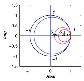
Proof: It follows from Corollary 1 that $(P_{\epsilon}+P_{MPC})\textit{{1}}=\textit{{1}}$. Moreover, since $\beta_{ij}\geq 0~{}(i\neq j)$, one has $R_{i}^{{}^{\prime}}(P_{\epsilon}+P_{MPC})=\sum_{j=1,j\neq i}^{N}\beta_{ij}=1-\beta_{ii}$. From Lemma 2, one obtains that all the eigenvalue of $P_{\epsilon}+P_{MPC}$ are located in the union of the $N$ discs

$$\cup_{i=1}^{n}\left\{z\in\mathbb{C}:|z-\beta_{ii}|\leq 1-\beta_{ii}\right\},$$ (27)

as shown in Fig. 2. Therefore, if $\beta_{ii}\in(0,1]$, then all the eigenvalues of the state matrix $P_{\epsilon}+P_{MPC}$ are in the open unit circle, except the simple eigenvalue $1$. Moreover, if the $\beta_{ii}$, $i=1,\ldots,N$ are arranged in non-ascending order, i.e. $0<\beta_{NN}\leq\beta_{N-1,N-1}\leq\ldots\leq\beta_{11}\leq 1$, as shown in Fig. 2, then the union of the $N$ discs (27) equals

$$\left\{z\in\mathbb{C}:|z-\beta_{NN}|\leq 1-\beta_{NN}\right\}.$$ (28)

Thus, taking Theorem 2 into consideration, one can conclude that average-consensus will be achieved asymptotically. $~{}~{}\hfill\blacksquare$

Remark 1

The assumptions $\beta_{ij}\geq 0~{}(i\neq j)$ and $\beta_{ii}\in(0,1]$ can be easily satisfied in general. Indeed, it can be numerically checked that in the $3$-dimensional space spanned by the parameters $H_{u}$, $H_{p}$, and $q$, there is a fairly large region in which these two assumptions are satisfied (such as the region corresponding to the common parameter settings $H_{u}\in[1,10]$, $H_{p}\in[H_{u},10]$, and $q\in[0.1,10]$). Moreover, the circle determined by (28) shrinks with increasing values of $\beta_{NN}~{}(\beta_{NN}\in(0,1))$, and the conditions given in Theorem 3 thus become more and more restrictive. Fortunately, for the common parameter settings $H_{u}\in[1,10]$, $H_{p}\in[H_{u},10]$, and $q\in[0.1,10]$, it can be shown by simulations that $\beta_{NN}$ is generally very close to zero when $\epsilon\leq 20/d_{\max}$, thereby reducing the conservativeness of the conditions of Theorem 3. In this way, the feasible range of the sampling period $\epsilon$ is significantly broadened. Indeed, when the routine state matrix $P_{\epsilon}$ is not discrete-time Hurwitz (which happens for $1/d_{\max}\leq\epsilon$ sa07 ), the MPC state matrix $P_{\epsilon}+P_{MPC}$ will still be discrete-time Hurwitz if $1/d_{\max}\leq\epsilon\leq\bar{\epsilon}$ where $\bar{\epsilon}$ is a certain threshold, typically much larger than $1/d_{\max}$. As shown in Theorem 3, this is due to the fact that the MPC consensus protocol is able to compress the cluster of eigenvalues and drive it to approach the origin when $\epsilon$ grows larger than the threshold value $1/d_{\max}$, as will be illustrated later, in the case study.

III.3 Case study

To vividly illustrate the advantages of the MPC consensus protocol, we present some simulation results comparing the convergence speeds obtained using the routine protocol given in (3) and the proposed MPC protocol given in (7), (14) for the particular case of all-to-all, balanced networks.

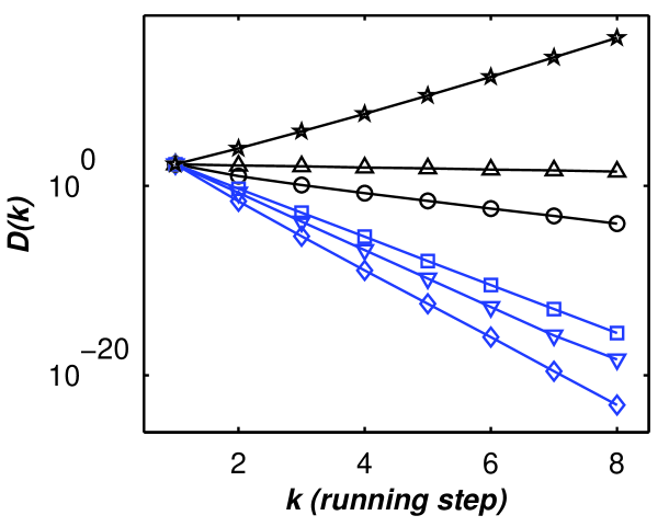
We first consider an all-to-all, symmetric network of $10$ nodes. Since the objective is to reach average-consensus, the instantaneous disagreement index is typically set as $D(k)\triangleq\|x(k)-\textbf{{1}}\bar{x}(0)\|_{2}^{2}$ and the consensus steps $T_{c}$ can be defined as the running steps required for $D(k)$ to reach a specified neighborhood of the origin and stay therein afterwards, i.e.

$$T_{c}(D_{c})=\min\left\{T\in\mathbb{R}^{+}:D(k)\leq D_{c},\,\forall k\geq T\right\},$$ (29)

where $D_{c}$ is a positive number defined as the consensus threshold, and $\|x\|_{2}=(x^{T}x)^{1/2}$. It is clear that $1/T_{c}(D_{c})$ gives a reasonable measurement of the consensus speed.

(a)	(b)

Figure 3: (Color online) (a) Comparison of the routine (black curves) and MPC (blue curves) protocols on the time evolution of the instantaneous disagreement index $D(k)$ corresponding to an all-to-all, symmetric network with different sampling periods $\epsilon$. Here, $l_{ij}=-1~{}(i\neq j)$ and $l_{ii}=N-1$. Case 1: $\epsilon=1/9=1/d_{\max}$, $\lozenge$: MPC, $\bigcirc$: routine protocol; Case 2: $\epsilon=0.03<1/d_{\max}$, $\bigtriangledown$: MPC, $\bigtriangleup$: routine protocol; Case 3: $\epsilon=2.00\gg 1/d_{\max}$, $\square$: MPC, $\bigstar$: routine protocol.   (b) Comparison of FDLA (black curves) and MPC (blue curves) protocols on a symmetric network with each off-diagonal entry $l_{ij}=l_{ji}~{}(i\neq j)$ selected randomly in $[-1,0]$. Here $\lozenge$: MPC; $+$: FDLA1; $\square$: FDLA2, $\epsilon=0.20$ and $d_{\max}\simeq 5$. In both (a) and (b), the MPC parameters are $N=10$, $H_{u}=2$, $H_{p}=4$, $q=2$, and the initial states $x_{i}(0),~{}i=1,\ldots,N$ are selected randomly in $[0,15]$.

As shown in Fig. 3(a), the addition of the predictive mechanism defined in (14), yields a drastic increase in convergence speed towards consensus. In particular, for $\epsilon\ll 1/d_{\max}$ ($d_{\max}=\max_{i}\left(l_{ii}\right)$), the convergence speed is increased more than $20$ times by using the proposed MPC protocol. Furthermore, even when the routine convergence conditions are violated, i.e. $\epsilon>1/d_{\max}$, it is observed that the MPC consensus protocol still allows asymptotic convergence with a high-speed.

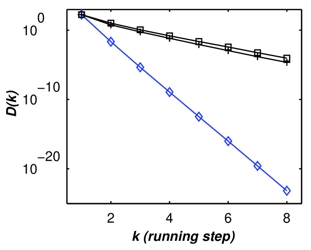
To further illustrate the advantages of the MPC protocol, comparison results of this latter protocol with the fastest distributed linear averaging (FDLA) protocols proposed in xi04 are presented in Fig. 3(b). More precisely, there are mainly three kinds of FDLA: if the dynamics of the considered network is determined by $x(k+1)=Wx(k)$, then

• in FDLA1, namely the best constant method, $W=I_{N}-\alpha L$ with $\alpha=2/(\lambda_{2}(L)+\lambda_{N}(L))$. FDLA1 is applicable only to symmetric networks;

• in FDLA2, namely the maximum-degree weight method, $W=I_{N}-\alpha L$ with $\alpha=1/d_{\max}$. FDLA2 is applicable only to symmetric networks;

• in FDLA3, namely the spectral norm minimization method, $W$ is the solution of the following spectral norm minimization problem:

  $$\begin{array}[]{c}\min_{W}~{}~{}~{}\|W-\textbf{{1}}\textbf{{1}}^{T}/N\|\\ s.t.~{}~{}~{}W\in\mathcal{E},~{}~{}\textbf{{1}}^{T}W=\textbf{{1}}^{T},~{}W\textbf{{1}}=\textbf{{1}}.\end{array}$$ (30)

It has been proven that the optimization problem (30) in FDLA3 is convex, thus FDLA3 can yield a global optimum $W^{*}$ for the consensus problemxi04 . Additionally, we note that FDLA2 is typically slower than FDLA1. The convergence properties of both FDLA1 and FDLA2 are described in xi04 .

It can be observed from Fig. 3(b) that the consensus speed of the proposed MPC protocol is much faster than that of FDLA1 and FDLA2, which is due to the larger degree of freedom allowed by the state matrix $W=P_{\epsilon}+P_{MPC}$. As to FDLA3, one can get that the optimum $W^{*}=\textbf{{1}}^{T}\textbf{{1}}/N$ for all-to-all link networks. As a consequence, $x(1)=Wx(0)=\textbf{{1}}\bar{x}$, namely, the disagreement index $D(k)$ will be zero in just one step, making FDLA3 the fastest possible consensus algorithm for all-to-all link networks. We have proven in Theorem 2 that the state matrix of the MPC protocol satisfies $\lim_{k\rightarrow\infty}(P_{\epsilon}+P_{MPC})^{k}=W^{*}$, provided that the matrix $P_{\epsilon}+P_{MPC}$ has a simple eigenvalue at $1$ and all its other eigenvalues in the open unit circle. Furthermore, considering all-to-all link networks, the constraints imposed in (30) are all fulfilled for $W=P_{\epsilon}+P_{MPC}$. Interestingly, we observe in Fig. 3 that $(P_{\epsilon}+P_{MPC})^{k}$ quickly approaches $W^{*}=\textbf{{1}}^{T}\textbf{{1}}/N$, which nicely illustrates the results presented in Theorem 2.

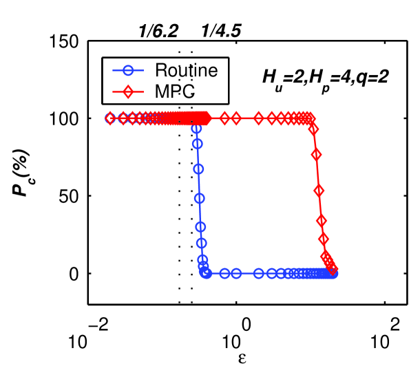
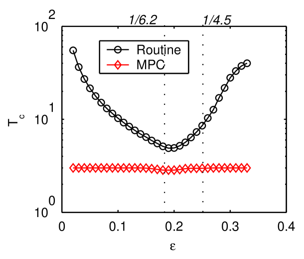
To further compare the convergence performances of the MPC and the routine protocols, we now generalize the above all-to-all, symmetric networks to an all-to-all, asymmetric, balanced networks with off-diagonal entries $a_{ij},~{}i\neq j$ selected randomly from $[-1,0]$. The corresponding time evolution of the instantaneous disagreement index $D(k)$ is fairly similar to the one presented in Fig. 3 for a symmetric all-to-all topology and is thus omitted here. Nevertheless, we show their associated ultrafast-convergence probabilities $P_{c}(D_{c})$ with respect to $\epsilon$ in Fig. 4(a). Here, $P_{c}(D_{c})$ denotes the ratio of ultrafast-convergence runs over $500$ runs for each $\epsilon$. A convergence run is considered ultrafast if the consensus threshold $D_{c}=0.01$ (see (29)) can be reached within $100$ steps. It can be observed that, with the assistance of a predictive mechanism, the ultrafast-convergence probability is significantly increased for each fixed value of $\epsilon$. Furthermore, the maximum feasible ultrafast-convergence sampling period $\epsilon$ is also sharply increased (more than $40$ times from our simulation results).

To further study the effects of the predictive mechanism and analyze its impact on the feasible convergence range of sampling periods $\epsilon$, we examine in Fig. 4(b) the evolution of the consensus steps $T_{c}(0.01)$ of these two strategies with respect to increasing values of $\epsilon$. In this comparison, for each value of $\epsilon$, $T_{c}$ denotes the average of the consensus steps corresponding to the successful convergence runs over a total of $500$ runs. It can be seen that, compared with the routine protocol, the MPC protocol allows for a significant increase in the consensus speed $1/T_{c}(0.01)$ (by a factor between $6$ and $20$ in our simulation results).

(a)	(b)

Figure 4: (Color online) (a): All-to-all link network’s ultrafast-convergence probability ($P_{c}(0.01)$); (b): consensus steps ($T_{c}(0.01)$). Comparison is addressed between the MPC (red curves) and routine (blue curves) protocols with different sampling periods $\epsilon$ and $500$ independent runs for each value of $\epsilon$. In these simulations, $H_{u}=2$, $H_{p}=4$, $q=2$, the consensus threshold $D_{c}=0.01$, each entry $l_{ij}(i\neq j)$ of $L$ is selected randomly in $[-1,0]$, and $x_{i}(0)~{}(i=1,\ldots,N)$ is selected randomly in $[0,15]$. The corresponding values of $d_{\max}$ lie in the range $[4.5,6.2]$. The vertical dotted lines correspond to the minimum and maximum values of $1/d_{\max}$.

(a)	(b)
(c)	(d)

Figure 5: (Color online) Evolution of the consensus steps ($T_{c}(10^{-7})$) of the MPC consensus protocol with respect to the control horizon $H_{u}$, the prediction horizon $H_{p}$ and the weighting parameter $q$. Here, the threshold $D_{c}=10^{-7}$, and the sampling period $\epsilon=0.05$.

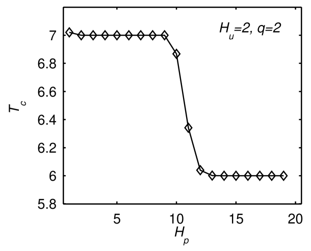
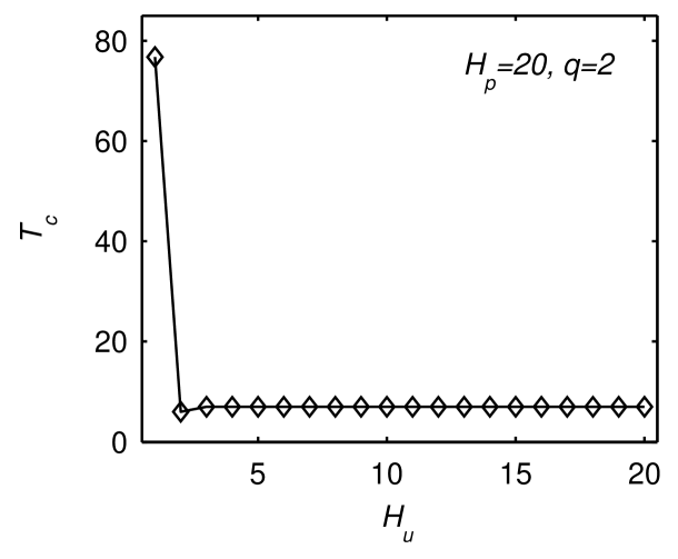
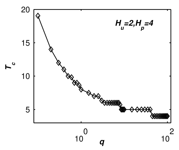
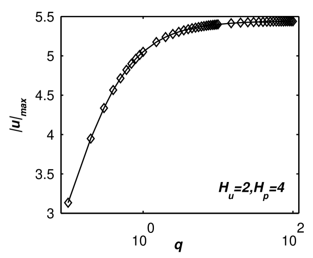
Since there are three crucial parameters determining the performances of the proposed MPC protocol, namely $H_{p}$, $H_{u}$ and $q$ (see (13)), statistical simulations have been carried out to investigate their individual influence on the convergence speed. The results of these simulations are shown in Fig. 5. One can observe that (i) the consensus speed $1/T_{c}(10^{-7})$ is enhanced with increasing values of the parameters $H_{p}$ (see Fig. 5(a)) or $q$ (see Fig. 5(c)); (ii) a global maximum of $1/T_{c}(10^{-7})$ exists at a value of $H_{u}$ (see Fig. 5(b)). Furthermore, $T_{c}(10^{-7})$ remains stable when $H_{u}$ exceeds a specified threshold (see also Fig. 5(b)).

Generally speaking, an increase in the values of $H_{p}$, $H_{u}$ and $q$, can improve the overall consensus performance. However, when their corresponding values exceed some thresholds, this improvement becomes negligible. Meanwhile the control efforts and computational burdens are still drastically increased (see Fig. 5(d)). Consequently, taking into consideration both computational complexity and consensus speed, one can find optimal parameter values according to the statistical simulation results depicted in Fig. 5.

(a)	(b)
(c)	(d)

Figure 6: (Color online) Eigenvalue distributions with respect to the sampling period $\epsilon.$ Blue $\bigcirc$ and red $+$ denote the eigenvalue distributions of $P_{\epsilon}$ and $P_{\epsilon}+P_{MPC}$ over $100$ runs, respectively. The black circle represents the unit circle in the complex plane. Here, $H_{u}=2$, $H_{p}=4$, $q=2$, and the entries $l_{ij},~{}j\neq i$ of $L$ are chosen randomly from $[-1,0]$. The corresponding values of $d_{\max}$ lie in the interval $[4.5,6.2]$ in this $100$-run simulation.

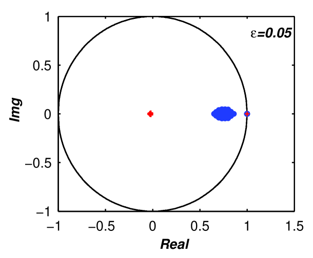
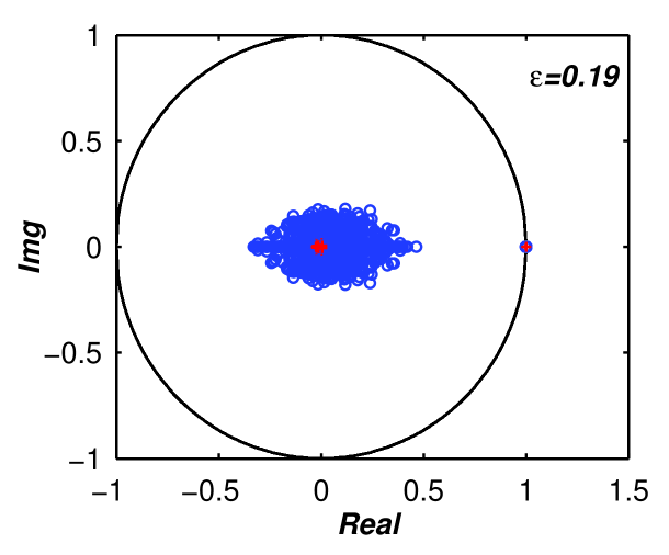
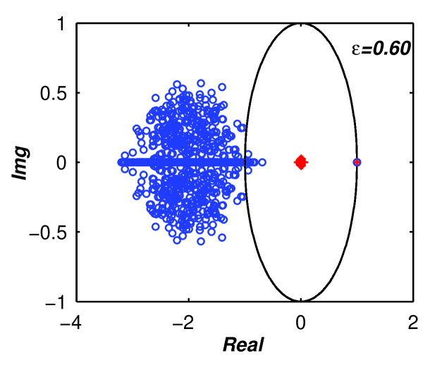
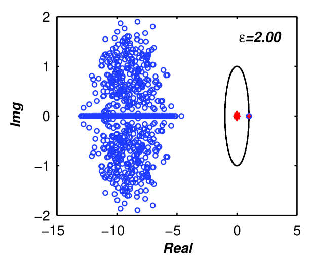
It is well known that the eigenvalue distribution of the state matrix associated with the considered consensus protocol, i.e. $P_{\epsilon}+P_{MPC}$, is closely linked to its performances. Therefore, to further study the proposed MPC protocol and better understand its ultrafast-convergence capability, we display the eigenvalue distributions of $P_{\epsilon}$ and $P_{\epsilon}+P_{MPC}$ in Fig. 6. These statistical simulations have been realized by considering $100$ different runs for a balanced, asymmetric network with entries $l_{ij},~{}i\neq j$ of the Laplacian matrix $L$ (appearing in the definition of the matrix $P_{\epsilon}$, see (5)) randomly selected from $[-1,0]$. For each run, we have considered $4$ different sampling period values for $\epsilon$. Based on these simulation results, an interesting phenomenon can be observed: the eigenvalue cluster of the matrix $P_{\epsilon}+P_{MPC}$ is always more compact around the origin than the counterpart cluster of $P_{\epsilon}$.

With these eigenvalue distributions, we can visualize the advantages of the MPC protocol more lively. Indeed, since the eigenvalue cluster of $P_{\epsilon}+P_{MPC}$ is always much smaller and closer to the origin of the complex plane than that of $P_{\epsilon}$, the MPC protocol generally has better consensus performance. When $\epsilon<1/d_{\max}$ ($\epsilon=0.05$, see Fig. 6(a)), the two eigenvalue clusters both remain inside the asymptotic stability region, i.e. the unit circle in the complex plane. However, since each eigenvalue of $P_{\epsilon}+P_{MPC}$ is much closer to the origin, the consensus speed is sharply increased in the case of the MPC protocol. Furthermore, when $\epsilon>1/d_{\max}$ ($\epsilon=0.60,2.00$, see Figs. 6(c) and (d)), some of the eigenvalues of $P_{\epsilon}$ escape the unit circle, making the disagreement function diverge, whereas all the eigenvalues of $P_{\epsilon}+P_{MPC}$ remain inside the unit circle, guaranteeing its asymptotic convergence. Finally, still worth mentioning is that the trivial eigenvalue of $P_{\epsilon}+P_{MPC}$, which corresponds to the eigenvector 1, always remains at $1$ irrespective of the value of $\epsilon$.

In summary, the advantages of the proposed MPC protocol are twofold: (i) enhancing the consensus speed associated with a fixed value of the sampling period $\epsilon$; (ii) enlarging the range of feasible convergence sampling periods. From the natural science point of view, the proposed MPC protocol, and especially its predictive mechanism, can be used to explain why individuals of bio-groups do not communicate with each others very frequently but only occasionally in a suitable manner during the whole dynamic process. From the industrial application point of view, due to the enlargement of the feasible range of the sampling periods, the use of the proposed MPC protocol allows for a significant reduction of the communication costs required to achieve a desired consensus speed.

IV Model predictive consensus protocol for partial link networks

In this section, we further compare the routine and the MPC consensus protocols in the more general case of partial link networks in which a pair of nodes is not necessarily connected. If we allow the topology of the network to be changed, in other words, if we allow the addition of some new edges in the graph, then the MPC protocol (14) proposed for all-to-all link networks can be used, and thus Theorems 1–3 and Corollary 1 remain valid. However, if we assume that the initial sparsity structure of the network is fixed, i.e. no new edge can be added in the graph, then we need to revise the MPC protocol (14) to obtain a new one suitable for this type of scenario. In the following sections, we first introduce a revised partial link, sparsity-preserving MPC consensus protocol. Afterwards, to support this latter protocol, we derive some necessary and sufficient condition guaranteeing its asymptotic convergence towards average-consensus. Finally, we provide simulation results for balanced partial link networks that show the advantages of this MPC protocol.

IV.1 Algorithm

In partial link networks, each node is allowed to communicate solely with its neighbors. To ensure that the communication structure of the network $G=(\mathcal{V},\mathcal{E},A)$ is preserved, one can slightly revise the additional MPC term $v(k)$ appearing in (7) to $v(k)=\Theta x(k)$, which leads to the following linear network dynamics

$$x(k+1)=P_{\epsilon}x(k)+\Theta x(k),$$ (31)

where $\Theta=\left\{\theta_{ij}\right\}_{i,j=1,\ldots,N}\in\mathbb{R}^{N\times N}$ satisfies the following relations:

1. the matrix $\Theta$ has the same sparsity structure as that of the network, i.e.

   $$(i,j)\notin\mathcal{E},~{}i\neq j\Rightarrow\theta_{ij}=0;$$ (32)

2. the matrix $\Theta$ will not change the symmetric property of the network, i.e.

   $$A^{T}=A\Rightarrow\Theta^{T}=\Theta;$$ (33)

3. $\Theta$ is balanced in the sense that

   $$\Theta\textit{{1}}=\Theta^{T}\textit{{1}}=\textbf{{0}}.$$ (34)

Note that these constraints are given to ensure feasibility of consensus by the proposed MPC protocol, which will be proven later. Fortunately, with these conditions, the degrees of freedom of $\Theta$ are reduced and the computational complexity of the proposed MPC algorithm is thus reduced.

By iterating the dynamic model given in (31), the evolution of the state of the $j^{th}$ agent can be predicted as

$$\begin{array}[]{l}x_{j}(k+m)=e_{j}(P_{\epsilon}+\Theta)^{m}x(k),\\ ~{}~{}~{}~{}~{}~{}~{}~{}~{}~{}~{}~{}~{}~{}~{}m=1,\cdots,H_{p};~{}j=1,\cdots,N,\end{array}$$ (35)

with $e_{j}\triangleq[0,\cdots,0,\underbrace{1}_{j^{th}},0,\cdots,0]_{1\times N}$. Similar to the all-to-all link case, the $m$-steps-ahead state difference of the $i^{th}$ and $j^{th}$ agents can be calculated by (9). However, in this partial link case, the $m$-steps-ahead network state difference vector, i.e. $\Delta x(k+m)$, is solely composed of the state differences of the neighboring pairs, i.e. $\Delta x(k+m)=\left(\mbox{col}\left(\Delta x_{i,j}(k+m)|(i,j)\in\mathcal{E}\right)\right)^{T}$. Note that if both $(i,j)$ and $(j,i)$ are in $\mathcal{E}$, only $x_{i,j}(k+m),~{}i>j$ will appear in $\Delta x(k+m)$.

Accordingly, the future evolution of the state difference can be predicted $H_{p}$ steps ahead:

$$\begin{array}[]{c}\Delta x(k+1)=\tilde{e}x(k+1),\\ \vdots\\ \Delta x(k+H_{p})=\tilde{e}x(k+H_{p}),\end{array}$$ (36)

with $\tilde{e}\triangleq\left(\mbox{col}\left(e^{T}_{i,j}|(i,j)\in\mathcal{E}\right)\right)^{T}$ and $e_{i,j}\triangleq e_{i}-e_{j}$. Note that if both $(i,j)$ and $(j,i)$ are in $\mathcal{E}$, only $e_{i,j},~{}i>j$ will appear in $\tilde{e}$. Then, substituting (31) into (36) yields

$$\begin{array}[]{c}\Delta X(k+1)\triangleq\left[\Delta x^{T}(k+1),\ldots,\Delta x^{T}(k+H_{p})\right]^{T}\\ =\tilde{E}X(k+1)=\tilde{E}\left[\left(P_{\epsilon}+\Theta\right)^{T},\ldots,\left(\left(P_{\epsilon}+\Theta\right)^{H_{p}}\right)^{T}\right]^{T}x(k),\end{array}$$ (37)

with $\tilde{E}=\mbox{diag}(\underbrace{\tilde{e},\ldots,\tilde{e}}_{H_{p}})$.

Analogous to what we have considered in the all-to-all link network case (12), the optimization index of the network here is designed as follows:

$$\begin{array}[]{c}J(\Theta,k)=\|\Delta X(k+1)\|_{Q}^{2}+\|\Theta x(k)\|_{R}^{2},\end{array}$$ (38)

where $Q$ and $R$ are positive definite symmetric weighting matrices. Thus, it follows from (37) and (38) that

$$J(\Theta,k)=x^{T}(k)J_{in}(\Theta)x(k)$$ (39)

with $J_{in}(\Theta)=\Gamma^{T}\tilde{E}^{T}Q\tilde{E}\Gamma+\Theta^{T}R\Theta$ and $\Gamma=\left[\left(P_{\epsilon}+\Theta\right)^{T},\ldots,\left(\left(P_{\epsilon}+\Theta\right)^{H_{p}}\right)^{T}\right]^{T}$.

Consequently, control law $\Theta$ can be derived as follows

$$\partial J_{in}(\Theta)/\partial\theta_{ij}|_{(i,j)\in\mathcal{E}}=0.$$ (40)

which leads to a set of polynomial equations. To solve this, Groebner basis methods can typically be used if the dimension of the problem to solve is not too high. Indeed, such methods allow to find all the solutions to a set of polynomial equations in several indeterminates, if the solution set consists of a finite set of isolated points co97 . Note that in the partial link case (31)–(40), the control horizon $H_{u}$ is always one. Certainly, one can extend $H_{u}$ by setting different values of $\Theta$ for different future steps; however, the computational burden will thereby increase remarkably. For this reason, multiple-step control horizons are not preferred for partial link networks.

IV.2 Analysis

In this section, based on Lemma 1, we provide a necessary and sufficient condition ensuring asymptotic convergence of the partial link MPC consensus protocol (see (31)–(34) and (40)) towards average-consensus.

Theorem 4

Consider a dynamical network $G_{x}$ whose dynamics are determined by the MPC protocol given in (31) and (40) and which satisfies the conditions (32) and (34). Then $\lim_{k\rightarrow\infty}x(k)=\textit{{1}}\bar{x}(0)$ (or average-consensus is reached asymptotically) if and only if either of the following two assumptions holds

1. $\rho(P_{\epsilon}+\Theta-\textbf{{1}}\textbf{{1}}^{T}/N)<1$;

2. the matrix $P_{\epsilon}+\Theta$ has a simple eigenvalue at $1$ and all its other eigenvalues in the open unit circle.

Proof: It follows from (19) and (34) that $(P_{\epsilon}+\Theta)\textit{{1}}=(P_{\epsilon}+\Theta)^{T}\textit{{1}}=\textit{{1}}$. Moreover, it can be seen from (32) that the sparsity structure of the matrix $P_{\epsilon}+\Theta$ corresponds to the one initially imposed by $\mathcal{E}$. Thus, taking into consideration of Lemma 1, the following equation holds:

$$\lim_{k\rightarrow\infty}x(k)=\lim_{k\rightarrow\infty}(P_{\epsilon}+\Theta)^{k}x(0)=\textit{{1}}\textit{{1}}^{T}/Nx(0)=\textit{{1}}\bar{x}(0)$$

if and only if either Assumption A6 or A7 is satisfied. $~{}~{}\hfill\blacksquare$

Remark 2

It will be illustrated later by simulations that Assumption A6 or A7 holds when $\epsilon$ grows to be much larger than $1/d_{\max}$. For partial link networks, one can generally compute a numerical solution (see (40)) rather than derive the corresponding analytical solution, thus the analysis cannot be formulated as thoroughly as for the all-to-all link case. However, the rationale of the predictive mechanism (31)–(40) is quite clear, i.e. the role of the routine part of the protocol ($P_{\epsilon}x(k)$) is to drive the state $x(k)$ to the average-consensus point $\textit{{1}}\bar{x}(0)$, while the role of the MPC part ($\Theta x(k)$) is to accelerate the consensus process by minimizing the future state difference between each neighboring pair in the network.

IV.3 Case study

In this section, we present some simulation results to compare the convergence speeds obtained using the routine consensus protocol given in (3), the FDLA protocol given in (30), and the proposed MPC protocol given in (31)–(34) and (40) for the case of partial link networks. Moreover, through these simulation results, one can also appreciate the difference in performances of the proposed MPC protocol for both all-to-all link and partial link networks.

(a)	(b)

Figure 7: (Color online) (a): balanced network topology; (b): time evolution of $D(k)=\|x(k)-\textbf{{1}}\bar{x}(0)\|_{2}^{2}$ when considering the MPC (blue curves), routine (black curves) and FDLA3 (red $+$ curve) protocols with different sampling periods $\epsilon$. Case 1:$\epsilon=1/3=1/d_{\max}$, $\lozenge$: MPC, $\bigcirc$: routine protocol; Case 2: $\epsilon=0.01<1/d_{\max}$, $\bigtriangleup$: routine protocol, $\bigtriangledown$: MPC; Case 3: $\epsilon=1.00>1/d_{\max}$, $\square$: MPC, $\bigstar$: routine protocol. In these simulations, $N=10$, $H_{u}=1$, $H_{p}=4$, $q=2$, and $x_{i}(0)~{}(i=1,\ldots,N)$ is selected randomly in $[0,15]$. $d_{\max}=\max_{i}\left(l_{ii}\right)=3$.

(a)	(b)

Figure 8: (Color online) (a): symmetric network topology; (b): time evolution of $D(k)=\|x(k)-\bar{x}(0)\textbf{{1}}\|_{2}^{2}$ when considering the MPC (blue curves), routine (black curve) and FDLA3 (red curves) protocols. Here $\lozenge$: MPC; $\bigtriangleup$: routine; $+$: FDLA1; $\square$: FDLA2; $\bigstar$: FDLA3. The MPC parameters are $N=10$, $H_{u}=1$, $H_{p}=4$, $q=2$, $x_{i}(0)~{}(i=1,\ldots,N)$ is selected randomly in $[0,15]$, $d_{\max}=\max_{i}\left(l_{ii}\right)=4$ and $\epsilon=0.1<1/d_{\max}$.

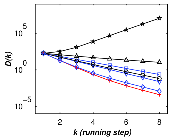
In these simulations, we have considered a $10$-node asymmetric partial link network whose topology is given in Fig. 7(a) (see sa04 ). For this partial link network $G=(\mathcal{V},\mathcal{E},A)$, the initial weights are fixed as follows: if $(i,j)\in\mathcal{E},~{}i\neq j$, then $a_{ij}=1$; otherwise, $a_{ij}=0$. As shown in Fig. 7(b), three different kinds of consensus strategies, i.e. the MPC (see (31)–(34) and (40)), routine (see (3)) and FDLA3 (see (30)) protocols, are compared. It can be observed that FDLA3 still holds the highest possible convergence speed while the addition of a predictive mechanism computed according to (31)–(34) and (40) yields a drastic increase in the convergence speed towards consensus compared with the routine protocol. Similar phenomena as those observed in the all-to-all link cases (see Fig. 3) can also be observed: for $\epsilon\ll 1/d_{\max}$, the convergence speed is increased sharply with this MPC protocol; for $\epsilon>1/d_{\max}$, the routine consensus protocol diverges while for $\epsilon$ values belonging to the interval $(1/d_{\max},\bar{\epsilon})$ with $\bar{\epsilon}\gg 1/d_{\max}$, the MPC protocol still converges with high-speed. Therefore, the feasible convergence range of $\epsilon$ is remarkably expanded by the proposed MPC protocol. More interestingly, for $\epsilon\rightarrow 1/d_{\max}$, the consensus speed of MPC approaches the fastest possible speed yielded by FDLA3 and is thus nearly maximized with the addition of a predictive mechanism.

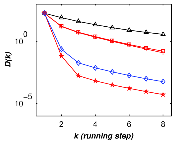
To illustrate the advantages of the MPC protocol more vividly, we present in Fig. 8(b) a comparison of the MPC, routine, FDLA1, FDLA2 and FDLA3 protocols (see (30)) when implemented on the symmetric network structure described in Fig. 8(a). In this case, the simulations were carried out with the fixed sampling period $\epsilon=0.1$. For this partial link network $G=(\mathcal{V},\mathcal{E},A)$, the initial weights are fixed as follows: if $(i,j)\in\mathcal{E},~{}i\neq j$, then $a_{ij}=1$; otherwise, $a_{ij}=0$. It can be observed from Fig. 8(b) that the consensus speeds of MPC and FDLA3 are much higher than those of FDLA1 and FDLA2, which is due to the larger degree of freedom of the corresponding state matrix $W$. Compared with MPC, FDLA3’s speed is even higher, since FDLA3 yields the global optimum $W^{*}$ in the fastest possible way xi04 . Moreover, it has been proven in Theorem 4 that consensus will be asymptotically reached provided that Assumption A6 or A7 holds. Also, it can be shown by simulations that Assumption A6 or A7 generally holds even when $\epsilon$ grows much larger than $1/d_{\max}$, and that $(P_{\epsilon}+\Theta)^{k}$ typically approaches $\textbf{{1}}\textbf{{1}}^{T}/N$ in just a few steps.

(a)	(b)

Figure 9: (Color online) (a): partial link network’s ultrafast-converge probability ($P_{c}(0.01)$) and (b): consensus steps ($T_{c}(0.01)$). Comparison is addressed between the MPC (red curves) and routine protocols (blue curves) with different sampling periods $\epsilon$ and $500$ independent runs for each $\epsilon$. For these simulations, $H_{u}=1$, $H_{p}=4$, $q=2$, the consensus threshold $D_{c}=0.01$, initial states $x_{i}(0),~{}i=1,\ldots,N$ are selected randomly in [0,15], and all non-zero entries $l_{ij}(i\neq j)$ of $L$ are selected randomly from $[-1,0]$. The corresponding values of $d_{\max}$ lie in the range $[0.9,2.7]$. The vertical dotted lines correspond to the minimum and maximum values of $1/d_{\max}$.

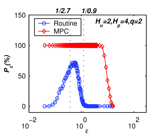
To compare the convergence performances of the MPC and routine consensus protocols for the asymmetric topology described in Fig. 7, we show their ultrafast-convergence probabilities $P_{c}(0.01)$ with respect to $\epsilon$ in Fig. 9(a). As previously, a convergence run is considered ultrafast if $D_{c}=0.01$ can be reached within $100$ steps. It can be observed that, with the assistance of the predictive mechanism, the ultrafast-convergence probability is significantly enhanced for all fixed values of $\epsilon$. Furthermore, the range of feasible convergence sampling periods is also sharply expanded (by a factor $10$ in our simulation results).

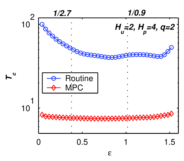
To further study the newly introduced predictive mechanism (31)–(40) and to analyze its impact on the feasible convergence range of sampling period $\epsilon$, we examine in Fig. 9(b) the evolution of the average value of the consensus steps $T_{c}(0.01)$ (see (29)) of these two strategies for the ultrafast-consensus runs. It can be seen that, compared with the routine consensus protocol, the use of MPC leads to a significant increase of the consensus speed $1/T_{c}(0.01)$ (by a factor between $5$ and $12$ in our simulation results).

Compared with the all-to-all link network case, the performance improvements of partial link networks are generally reduced. This should be attributed to the fact that each node of an all-to-all link network can use the information of all the other ones for prediction, whereas the information flow in a partial link network is constrained by its topology. Moreover, another interesting phenomenon deserving notice is that, for the routine consensus protocol, the $P_{c}(0.01)$ curve starts with a very low value for small $\epsilon$, ascends to the peak (which correspond to about $80\%$) in the left half of the $d_{\max}$ zone and finally returns to zero very quickly within the right half of the $d_{\max}$ zone. This phenomenon should also be attributed to the information flow constraints imposed by the partial link topology and the fact that the routine protocol convergence speed is maximized when $\epsilon=1/d_{\max}$ (see FDLA2 in xi04 ).

(a)	(b)
(c)	(d)

Figure 10: (Color online) partial link network’s eigenvalue distribution with respect to the sampling period $\epsilon$. Blue $\bigcirc$ and red $+$ denote the eigenvalue distributions of $P_{\epsilon}$ and $(P_{\epsilon}+P_{MPC})$ over $100$ runs, respectively. The black circle represents the unit circle in the complex plane. Here, $H_{u}=1$, $H_{p}=4$, $q=2$. According to the network topology (see Fig. 7(a)), each non-zero entry $l_{ij}~{}(i\neq j)$ of $L$ is selected randomly in $[-1,0]$, and it is calculated that $d_{\max}\in[0.9,2.7]$ in this $100$-run simulation.

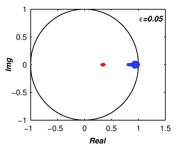
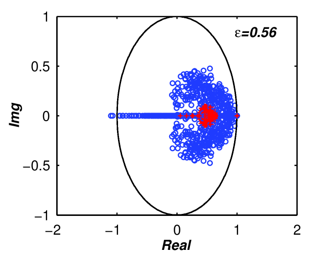
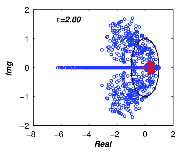
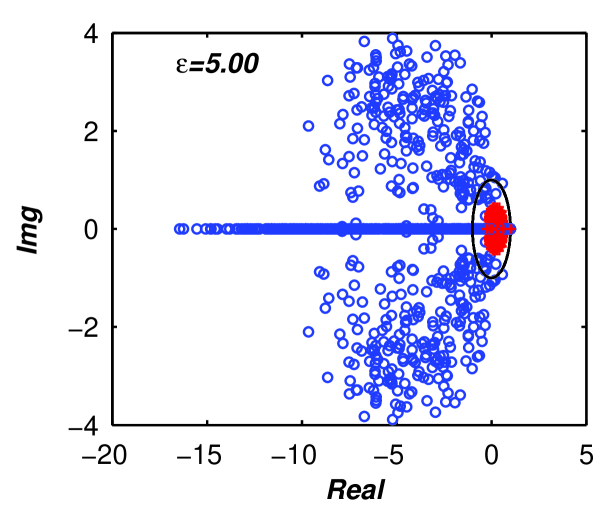
To investigate MPC’s ultrafast-consensus capabilities even more carefully, we compare the distribution of eigenvalues for the two matrices $P_{\epsilon}$ and $P_{\epsilon}+P_{MPC}$ in Fig. 10. Similar to the all-to-all link network case, these statistical simulations have been realized by considering $100$ different runs for an asymmetric balanced network with the topology shown in Fig. 7(a). In these simulations, each non-zero entry $l_{ij},~{}i\neq j$ of $L$ is selected randomly in $[-1,0]$ at each run. For each run, we have considered $4$ different sampling period values for $\epsilon$. Based on these simulation results, similar phenomena to those reported in the all-to-all link network case (see Fig. 6) can be observed. Compared with the eigenvalue-cluster of $P_{\epsilon}$, the one of $P_{\epsilon}+P_{MPC}$ is always much smaller and closer to the origin, which explains the overall higher consensus speed of the MPC protocol. Moreover, if $\epsilon$ approaches $1/d_{\max}$ ($\epsilon=0.56$, Fig. 10(b)), the eigenvalue-cluster of $P_{MPC}$ approaches that of $P_{\epsilon}$, and the overlapping area of these two clusters increases. When $\epsilon$ is increased beyond $1/d_{\max}$ (see Fig. 10(c) and (d)), some of the eigenvalues of $P_{\epsilon}$ start escaping the unit circle, making the disagreement function diverge, whereas the whole eigenvalue cluster of $P_{\epsilon}+P_{MPC}$ remains inside the unit circle, which ensures its convergence. Moreover, still worth mentioning is that the eigenvalue of $P_{\epsilon}+P_{MPC}$, which corresponds to the eigenvector 1, always remains at $1$ irrespective of the value of $\epsilon$. This is due to the balanced constraints (34) imposed on the MPC matrix $\Theta$.

Finally, as shown in Fig. 10, there are also obvious differences between the all-to-all link and partial link network cases, i.e. the eigenvalue cluster of the former is much smaller and closer to the origin than that of the latter. This difference is also attributed to the reduced information flow imposed by the partial link network topology (see Fig. 7(a)). Consequently, the improvements resulting from the use of the MPC prediction mechanism are reduced in the partial link network scenario.

V Conclusion

In this paper, in order to reveal the role of predictive mechanisms in many natural bio-groups, we have added a certain kind of predictive mechanism to the routine consensus protocol to design a novel MPC protocol. Furthermore, we have presented mathematical analysis as well as statistical simulation results to show the improvement of consensus performances through the use of such a protocol.

In particular, we have compared the routine, FDLA and MPC consensus protocols in the general cases of symmetric and asymmetric, balanced all-to-all link networks, and asymmetric balanced partial link networks. The comparisons have led to the following two conclusions: (i) the convergence speed towards consensus can be significantly increased to approach the global optimum via the predictive mechanism, namely, even short-term inspection of the future can produce a significant increase in convergence speed; (ii) the sampling period range guaranteeing convergence is increased sharply by this predictive mechanism, giving the MPC protocol the potential to effectively save communication energy. These advantages have been explained through mathematical analysis of the eigenvalue distributions.

To investigate the predictive mechanism more analytically, we have provided some necessary and sufficient conditions guaranteeing asymptotic convergence towards average-consensus for all-to-all link and partial link networks, respectively. In particular, we have considered the special case of balanced all-to-all link networks and showed that the proposed MPC protocol can effectively compress the eigenvalue cluster of the system state matrix and drive it back towards the origin of the complex plane when the sampling period is increased beyond the routine convergence threshold. In the special case of symmetric all-to-all link networks, we proved that the corresponding state matrix $P_{\epsilon}+P_{MPC}$ shares the same eigenvectors as the matrix $P_{\epsilon}$.

Furthermore, to verify the generality of these conclusions, we have also applied the proposed MPC protocol to two popular complex network models, the Vicsek model vi95 and the Attractive/Repulsive model ga03 . The corresponding results presented in zh07 show that predictive protocol outperforms the routine protocol when taking into consideration both the consensus speed and the communication cost.

For natural science, the contribution of this work lies in its ability to explain why networks of biological flocks/swarms/schools such as firefly and deep-sea fish groups do not communicate very frequently all along but only occasionally during the whole dynamical process. From the industrial application point of view, the value of this work is two-fold: the consensus speed can be significantly enhanced, and the communication energy or cost can be reduced remarkably. All these merits are at the cost of giving the agents the capabilities of making predictions, which can be efficiently achieved based on currently available information. This work is just a first attempt aiming at achieving ultrafast-consensus by injecting a prediction mechanism into classical consensus algorithms such as the routine consensus protocol, and we hope it will open up new avenues in biological and industrial applications.

Finally, we stress that the presented results rely on a centralized control approach. In ongoing works, we are developping a decentralized version of these MPC consensus algorithms.

.1 Proof of Theorem 1

First, it is easy to see that the matrix $P_{U_{{}_{H_{p}N\times H_{u}N}}}$ in (8) has the following structure

$$P_{U}=\left[\begin{array}[]{llll}I_{N}&&&\\ P_{\epsilon}&I_{N}&&\\ \vdots&&\ddots&\\ P_{\epsilon}^{H_{u}-1}&P_{\epsilon}^{H_{u}-2}&\ldots&I_{N}\\ P_{\epsilon}^{H_{u}}&\ldots&P_{\epsilon}^{2}&P_{\epsilon}+I_{N}\\ \vdots&&\vdots&\vdots\\ P_{\epsilon}^{H_{p}-1}&\ldots&P_{\epsilon}^{H_{p}-H_{u}+1}&\begin{array}[]{l}P_{\epsilon}^{H_{p}-H_{u}}\\ +P_{\epsilon}^{H_{p}-H_{u}-1}\\ +\ldots+I_{N}\end{array}\end{array}\right].$$ (41)

Furthermore, we have

$$P_{XE}\eta_{i}=\left[\lambda_{i}\eta_{i}^{T},\ldots,\lambda_{i}^{H_{p}}\eta_{i}^{T}\right]^{T}.$$

The weighting matrices $Q,R$ are selected as in (13). Straightforward calculations then show that

$$\begin{array}[]{l}P_{UE}^{T}QP_{XE}\eta_{i}=\\ \left[\left.g_{1}\right._{q}^{H_{p},H_{u}}\left(\lambda_{i}\right)\eta_{i}^{T},\ldots,\left.g_{H_{u}}\right._{q}^{H_{p},H_{u}}\left(\lambda_{i}\right)\eta_{i}^{T}\right]_{H_{u}N\times 1}^{T},\end{array}$$ (42)

where $\left.g_{1}\right._{q}^{H_{p},H_{u}}\left(\lambda_{i}\right),\ldots,\left.g_{H_{u}}\right._{q}^{H_{p},H_{u}}\left(\lambda_{i}\right)$ denote polynomial functions of $\lambda_{i}$ with orders determined by $H_{p}$, $H_{u}$ and coefficients determined by $q$.

On the other hand, for $H_{u}$ arbitrary scalars $\gamma_{i}\in\mathbb{R}~{}(i=1,\ldots,H_{u})$, one has $P_{UE}\left[\gamma_{1}\eta_{i}^{T},\ldots,\gamma_{H_{u}}\eta_{i}^{T}\right]^{T}=$ $\left[\left.h_{1}\right._{\gamma_{1},\ldots,\gamma_{H_{u}},q}^{H_{p},H_{u}}\left(\lambda_{i}\right)\eta_{i}^{T},\right.\ldots,\left.\left.h_{H_{u}}\right._{\gamma_{1},\ldots,\gamma_{H_{u}},q}^{H_{p},H_{u}}\left(\lambda_{i}\right)\eta_{i}^{T}\right]_{H_{u}N\times 1}^{T}$, where $\left.h_{1}\right._{\gamma_{1},\ldots,\gamma_{H_{u}},q}^{H_{p},H_{u}}\left(\lambda_{i}\right),\ldots,\left.h_{H_{u}}\right._{\gamma_{1},\ldots,\gamma_{H_{u}},q}^{H_{p},H_{u}}\left(\lambda_{i}\right)$ are the corresponding polynomial functions with orders determined by $H_{p}$, $H_{u}$ and coefficients determined by $\gamma_{1},\ldots,\gamma_{H_{u}}$ and $q$.

Since $P_{\epsilon}$ is symmetric and $Q=qI$, $R=I$, it follows that

$$\begin{array}[]{c}(P_{UE}^{T}QP_{UE}+R)\left[\gamma_{1}\eta_{i}^{T},\ldots,\gamma_{H_{u}}\eta_{i}^{T}\right]^{T}={}{}{}{}{}{}{}{}{}{}{}{}\\ \left[\left.f_{1}\right._{\gamma_{1},\ldots,\gamma_{H_{u}},q}^{H_{p},H_{u}}\left(\lambda_{i}\right)\eta_{i}^{T}\right.,\ldots,\left.\left.f_{H_{u}}\right._{\gamma_{1},\ldots,\gamma_{H_{u}},q}^{H_{p},H_{u}}\left(\lambda_{i}\right)\eta_{i}^{T}\right]_{H_{u}N\times 1}^{T},\end{array}$$ (43)

where $\left.f_{1}\right._{\gamma_{1},\ldots,\gamma_{H_{u}},q}^{H_{p},H_{u}}\left(\lambda_{i}\right),\ldots,\left.f_{H_{u}}\right._{\gamma_{1},\ldots,\gamma_{H_{u}},q}^{H_{p},H_{u}}\left(\lambda_{i}\right)$ are the corresponding polynomial functions of $\lambda_{i}$ with orders determined by $H_{p}$, $H_{u}$ and coefficients by $\gamma_{1},\ldots,\gamma_{H_{u}}$ and $q$.

For fixed values of $H_{u}$, $H_{p}$, $q$ and $\lambda_{i}$, it can be verified that $\left.g_{i}\right._{q}^{H_{p},H_{u}}\left(\lambda_{i}\right),~{}i=1,\ldots,H_{u}$ corresponds to a constant scalar denoted by $g_{i}$, and $\left.f_{i}\right._{\gamma_{1},\ldots,\gamma_{H_{u}},q}^{H_{p},H_{u}}\left(\lambda_{i}\right),~{}i=1,\ldots,H_{u},$ corresponds to a linear function of $\gamma_{1},\ldots,\gamma_{H_{u}}$ denoted by $f_{i}\left(\gamma_{1},\ldots,\gamma_{H_{u}}\right)$. As a result, the following set of $H_{u}$ linear equations

$$f_{i}(\gamma_{1},\ldots,\gamma_{H_{u}})=g_{i},~{}i=1,\ldots,H_{u},$$ (44)

always possesses a unique solution $\gamma_{1}=\gamma_{1}^{*},\ldots,\gamma_{H_{u}}=\gamma_{H_{u}}^{*}$. With this particular solution, the right-hand sides of (42) and (43) are equal, i.e.

$$P_{UE}^{T}QP_{XE}\eta_{i}=(P_{UE}^{T}QP_{UE}+R)\left[\gamma_{1}^{*}\eta_{i}^{T},\ldots,\gamma_{H_{u}}^{*}\eta_{i}^{T}\right]^{T}.$$

Using this last equality, the definition of $P_{MPC}$ given in (15) yields

$$\begin{array}[]{l}P_{MPC}\eta_{i}=-\left[I_{N},\mathbf{0}_{N},\ldots,\mathbf{0}_{N}\right]_{N\times H_{u}N}\left(P_{UE}^{T}QP_{UE}+R\right)^{-1}\\ \cdot P_{UE}^{T}QP_{XE}\eta_{i}=-\left[I_{N},\mathbf{0}_{N},\ldots,\mathbf{0}_{N}\right]\left[\gamma_{1}^{*}\eta_{i}^{T},\ldots,\gamma_{H_{u}}^{*}\eta_{i}^{T}\right]^{T}\\ ~{}~{}~{}~{}~{}~{}~{}~{}~{}~{}~{}~{}~{}~{}~{}~{}~{}=-\gamma_{1}^{*}\eta_{i}.\\ \end{array}$$

Therefore, $P_{\epsilon}$ and $P_{MPC}$ share the same eigenvector $\eta_{i},~{}i=1,\ldots,N$ and the corresponding eigenvalue $\nu_{i}$ of $P_{MPC}$ equals $-\gamma_{1}^{*}$ where $\gamma_{1}^{*}$ is different for each fixed value of $\lambda_{i}$. This completes the proof of the property 1) in Theorem 1.

On the other hand, recall the definition $E\triangleq\mbox{diag}(e,\ldots,e)_{H_{p}N(N-1)/2\times H_{p}N}$ and take into consideration that $Q=qI$. We have $E^{T}QE=diag(\underbrace{\Xi,\ldots,\Xi}_{H_{p}})$ with $\Xi\in\mathbb{R}^{N\times N}$ being a symmetric matrix. Then, $E^{T}QEP_{X}=\left[\left(\Xi P_{\epsilon}\right)^{T},\ldots,\left(\Xi P_{\epsilon}^{H_{p}}\right)^{T}\right]^{T}=\left[P_{\epsilon}\Xi,\ldots,P_{\epsilon}^{H_{p}}\Xi\right]^{T}$ which leads to $P_{U}^{T}E^{T}QEP_{X}=\left[h_{1}\left(P_{\epsilon},\Xi\right),\ldots,h_{H_{u}}\left(P_{\epsilon},\Xi\right)\right]^{T}_{H_{u}N\times N}$, where $h_{i}\left(P_{\epsilon},\Xi\right)~{}(i=1,\ldots,H_{u})$ are polynomial functions of $P_{\epsilon}$ and $\Xi$. Due to the symmetry of $P_{\epsilon}$ and $\Xi$, $h_{i}(P_{\epsilon},\Xi)~{}(i=1,\ldots,H_{u})$ are also symmetric. Analogously, $P_{UE}^{T}QP_{UE}+R=\left\{\psi_{i,j}(P_{\epsilon})\right\},~{}i,j=1,\ldots,H_{u}$, where $\psi_{i,j}(P_{\epsilon})$ are polynomial functions of $P_{\epsilon}$. Due to the symmetry of $P_{\epsilon}$, $\psi_{i,j}(P_{\epsilon}),~{}i,j=1,\ldots,H_{u}$ are also symmetric, thus $(P_{UE}^{T}QP_{UE}+R)^{-1}$ contains $H_{u}\times H_{u}$ symmetric matrices $\varphi_{i,j}(P_{\epsilon})$ and $-\left[I_{N},\mathbf{0}_{N},\ldots,\mathbf{0}_{N}\right]_{N\times H_{u}N}(P_{UE}^{T}QP_{UE}+R)^{-1}=-\left[\varphi_{1,1}(P_{\epsilon}),\ldots,\varphi_{1,H_{u}}(P_{\epsilon})\right]$. Accordingly, it is easy to see from (15) that $P_{MPC}=-\sum_{i=1}^{H_{u}}\varphi_{1,i}(P_{\epsilon})\cdot h_{i}(P_{\epsilon},\Xi)$. Since $\varphi_{1,i}(P_{\epsilon})$ and $h_{i}(P_{\epsilon},\Xi)$ are both symmetric, one has that $P_{MPC}$ is also symmetric. This completes the proof of the property 2) in Theorem 1.

.2 Proof of the second part of Lemma 1

Necessity: (22) $\Rightarrow$ A1 and A3 (see xi04 ).

Notice that $\lim_{k\rightarrow\infty}W^{k}$ exists if and only if there is a non-singular matrix $T$ such that

$$\lim_{k\rightarrow\infty}W=\lim_{k\rightarrow\infty}T\left[\begin{array}[]{cc}I_{m}&\mathbf{0}\\ \mathbf{0}&\mathbf{Z}\end{array}\right]T^{-1},$$

where $\mathbf{Z}$ is a convergent matrix, i.e. $\rho(\mathbf{Z})<1$. One then has that

$$\begin{array}[]{c}\lim_{k\rightarrow\infty}W^{k}=\lim_{k\rightarrow\infty}T\left[\begin{array}[]{cc}I_{m}&\mathbf{0}\\ \mathbf{0}&\mathbf{Z}^{k}\end{array}\right]T^{-1}\\ =T\left[\begin{array}[]{cc}I_{m}&\mathbf{0}\\ \mathbf{0}&\mathbf{0}\end{array}\right]T^{-1}=\sum_{i=1}^{m}\gamma_{i}\zeta_{i},\end{array}$$ (45)

where $\gamma_{i}$ and $\zeta_{i}^{T}~{}(i=1,\ldots,N)$ are columns of $T$ and rows of $T^{-1}$, respectively. Since each $\gamma_{i}\zeta_{i}^{T}$ is a rank-one matrix and $\sum_{i=1}^{N}\gamma_{i}\zeta_{i}=TT^{-1}=I_{N}$ has rank $N$, the matrix $\sum_{i=1}^{m}\gamma_{i}\zeta_{i}$ must have rank $m$. Comparing (22) and (45) gives $m=1$ and $\gamma_{1}\zeta_{1}^{T}=\textbf{{1}}\textbf{{1}}^{T}/N$, which implies that both $\gamma_{1}$ and $\zeta_{1}$ are multiples of 1. In other words, $1$ is a simple eigenvalue of $W$ and 1 is its associated left and also right eigenvectors, i.e. Assumptions A1 and A3 hold.

Sufficiency: A1 and A3 $\Rightarrow$ (22).

If A1 and A3 hold, then there is a nonsingular matrix $T$ such that

$$W=T\left[\begin{array}[]{cc}1&\mathbf{0}\\ \mathbf{0}&\mathbf{Z}\end{array}\right]T^{-1},$$

where $\mathbf{Z}$ is a convergent matrix, i.e. $\rho(\mathbf{Z})<1$ (this can be derived using the Jordan canonical form st88 ). Let $\gamma_{1},\ldots,\gamma_{N}$ be the columns of $T$ and $\zeta_{1}^{T},\ldots,\zeta_{N}^{T}$ be the rows of $T^{-1}$. Then, we have

$$\begin{array}[]{c}\lim_{k\rightarrow\infty}W^{k}=\lim_{k\rightarrow\infty}T\left[\begin{array}[]{cc}1&\mathbf{0}\\ \mathbf{0}&\mathbf{Z}^{k}\end{array}\right]T^{-1}\\ =T\left[\begin{array}[]{cc}1&\mathbf{0}\\ \mathbf{0}&\mathbf{0}\end{array}\right]T^{-1}=\gamma_{1}\zeta_{1}.\end{array}$$

It can be seen from Assumption A1 and the Jordan canonical form st88 that $\gamma_{1}$ and $\zeta_{1}$ can be selected as normalized column eigenvector $\textbf{{1}}\cdot 1/\sqrt{N}$ and row eigenvector $\textbf{{1}}^{T}\cdot 1/\sqrt{N}$, respectively (note that $\gamma_{1}$ and $\zeta_{1}$ are not unique, but their product is unique), which implies (22) immediately.

References

- (1) Corresponding author, mc274@leicester.ac.uk
- (2) S. Marinez, J. Cortes and F. Bullo, “Motion coordination with distributed information,” IEEE Control System Magazine, vol. 27, no. 4, pp. 75–88, 2007.
- (3) E. O. Budrene and H. Berg, “Dynamics of formation of symmetrical patterns by chemotactic bacteria,” Nature, vol. 376, pp. 49–53, 1995.
- (4) L. You, R. S. Cox III, R. Weiss and F. H. Arnold, “Programmed population control by cell-cell communication and regulated killing,” Nature, vol. 428, pp. 868–871, 2004.
- (5) R. D. Astumian and M. Bier, “Fluctuation driven ratchets: molecular motors,” Physical Review Letters, vol. 72, no. 11, pp. 1766–1769, 1994.
- (6) T. Vicsek, A. Czirók, E. Ben-Jacob, I. Cohen and O. Shochet, “Novel type of phase transition in a system of self-driven particles,” Physcial Review Letters, vol. 75, no. 6, pp. 1226–1229, 1995.
- (7) G. Grégoire and H. Chaté, “Onset of collective and cohesive motion,” Physcial Review Letters, vol. 92, no. 2, pp. 025702, 2004.
- (8) M. Aldana, V. Dossetti, C. Huepe, V. M. Kenkre, and H. Larralde,“Phase transitions in systems of self-propelled agents and related network models,” Physcial Review Letters, vol. 98, pp. 095702, 2007.
- (9) R. Olfati-Saber and R. Murray, “Consensus problems in networks of agents with switching topology and time-delays,” IEEE Transactions on Automatic Control, vol. 49, no. 9, pp. 1520–1533, 2004.
- (10) W. Ren, R. W. Beard and E. M. Arkins, “Information consensus in multivehicle cooperative control,” IEEE Control System Magazine, vol. 71, no. 2, pp. 71–82, 2004.
- (11) I. F. Akyildiz, W. Su, Y. Sankarasubramaniam, and E. Cayirci, “Wireless sensor networks: a survey,” Computers Network, vol. 38, no. 4, pp. 393–422, 2002.
- (12) P. Ogren, E. Fiorelli, and N. E. Leonard, “Cooperative control of mobile sensor networks:Adaptive gradient climbing in a distributed environment,” IEEE Transactions on Automatic Control, vol. 49, no. 8, pp. 1292–1302, 2004.
- (13) T. Arai, E. Pagello, and L. E. Parker, “Guest editorial advances in multirobot systems,” IEEE Transactions Robotics and Automation, vol. 18, no. 5, pp. 655–661, 2002.
- (14) M. Fiedler, “Algebraic connectivity of graphs,” Czechoslovak Mathematical Journal, vol. 23, no. 98, pp. 298–305, 1973.
- (15) R. Olfati-Saber and R. Murray, “Consensus and cooperation in networked multi-agent systems,” Proceedings of IEEE, vol. 95, no. 1, pp. 215–233, 2007.
- (16) R. Olfati-Saber, “Ultrafast consensus in small-world networks,” in Proceedings of American Control Conference, June 2005, pp. 2371–2378.
- (17) S. H. Strogatz, “Exploring complex networks,” Nature, vol. 410, pp. 268–276, 2001.
- (18) L. Xiao, S. Boyd, “Fast linear iterations for distributed averaging,” Systems Control Letters, vol. 53, no. 1, pp. 65–78, 2004.
- (19) W. Yang, L. Cao, X. F. Wang, and X. Li, “Consensus in a heterogeneous influence network,” Physical Review E, vol. 74, pp. 037101, 2006.
- (20) E. F. Woods, “Electronic prediction of swarming in bees,” Nature, vol. 184, no. 4690, pp. 842–844, 1959.
- (21) P. R. Montague, P. Dayan, C. Person, and T. J. Sejnowski, “Bee foraging in uncertain environments using predictive hebbian learning,” Nature, vol. 377, pp. 725–728, 1995.
- (22) J. A. Gottfried, J. O. Doherty and R. J. Dolan, “Encoding predictive reward value in human amygdala and orbitofrontal cortex,” Science, vol. 301, no. 5636, pp. 1104–1107, 2003.
- (23) C. Summerfield, T. Egner, M. Greene, E. Koechlin, J. Mangles and J. Hirsch, “Predictive codes for forthcoming perception in the frontal cortex,” Science, vol. 314, no. 5803, pp. 1311–1314, 2006.
- (24) D. Melcher, “Predictive remapping of visual features precedes saccadic eye movements,” Nature Neuroscience, vol. 10, no. 7, pp. 903–907, 2007.
- (25) R. A. Horn and C. R. Johnson, Matrix Analysis, Cambridge University Press, Cambridge, 1990.
- (26) B. A. Asner, “On the total nonnegativity of the Hurwitz matrix,” SIAM Journal of Applied Mathematics, vol. 18, no. 2, pp. 407–414, 1970.
- (27) D. Cox, J. Little and D. Q. Shea, Ideals, Varieties and Algorithms, Springer-Velag, New York, 1997.
- (28) V. Gazi and K. M. Passino, “Stability analysis of swarms,” IEEE Transactions on Automatic Control, vol. 48, no. 4, pp. 692–697, 2003.
- (29) H. T. Zhang, M. Z. Q. Chen and T. Zhou, “Predictive protocol of flocks with small-world connection pattern,” arXiv, 0709.0380, 2007.
- (30) G. Strang, Linear Algebra and Its Applications, Thomson Learning Inc., 1988.