Generalised thermostatistics using hyperensembles

Abstract

The hyperensembles, introduced by Crooks in a context of non-equilibrium statistical physics, are considered here as a tool for systems in equilibrium. Simple examples like the ideal gas, the mean-field model, and the Ising interaction on small square lattices, are worked out to illustrate the concepts.

1 Introduction

The starting point of superstatistics BC03 ; BC07 is the assumption that the inverse temperature $\beta$ of the Boltzmann-Gibbs distribution

$$q_{\beta}(x)=\frac{1}{Z(\beta)}e^{-\beta H(x)}$$ (1)

may itself be a fluctuating quantity, governed by a probability density $f(\beta)$. The resulting probability distribution is then determined by

$$p_{f}(x)=\int_{0}^{\infty}{\rm d}\beta\,f(\beta)q_{\beta}(x).$$ (2)

The choice of the hyperdistribution $f(\beta)$ (called the entropic distribution in CGE07 ) depends on the application at hand. Recently, Crooks CGE07 suggested that this distribution should be determined by means of the Maximum Entropy Principle (MEP) because, in general, information is lacking about what choice of $f(\beta)$ is appropriate. Additional constraints, introduced when applying the MEP, then lead to a parametrised family of probability distributions. The latter he called a hyperensemble.

The choice of constraints is crucial. Crooks proposes to use three constraints: the normalisation, the mean energy and the mean entropy. The result of applying the MEP is that the hyperdistribution is of the form

$$f(\beta)=\frac{c(\beta)}{Z(\theta,\lambda)}\exp\left(\lambda\check{S}(\beta)-\theta\langle H\rangle_{\beta}\right).$$ (3)

Here, $\theta$ is the Lagrange multiplier controlling the mean energy, $\lambda$ controls the mean entropy. The canonical entropy is denoted $\check{S}(\beta)$ to distinguish it from the entropy of the hyperensemble. The normalisation is given by

$$Z(\theta,\lambda)=\int_{0}^{\infty}c(\beta){\rm d}\beta\,\exp\left(\lambda\check{S}(\beta)-\theta\langle H\rangle_{\beta}\right).$$ (4)

The intention of Crooks is to use the notion of hyperensembles to study systems out of equilibrium. The present paper shows the usefulness of hyperensembles as a unifying concept for systems in equilibrium. In this context the parameter $\lambda$ plays no important role and may be taken equal to 1.

2 The ideal gas

Consider only the momenta $p_{1},p_{2},\cdots,p_{N}$ of an ideal gas containing $N$ particles. The Hamiltonian is

$$H(p)=\frac{1}{2m}\sum_{n=1}^{N}\sum_{\alpha=1}^{3}p_{n\alpha}^{2}.$$ (5)

The canonical probability distribution is

$$q_{\beta}(p)=\frac{1}{(2\pi mk_{B}T)^{3N/2}}e^{-\beta H(p)}.$$ (6)

The entropy and energy equal

$$\check{S}(\beta)=-\frac{3N}{2}\ln\beta,\qquad\qquad\langle H\rangle_{\beta}=\frac{3N}{2}\beta^{-1}.$$ (7)

After optimisation, the hyperdistribution becomes

$$f(\beta)=\frac{c(\beta)}{Z(\theta)}\exp\left(-\frac{3N}{2}\ln\beta-\theta\frac{3N}{2\beta}\right).$$ (8)

This is the inverse Gamma distribution, also called the inverse $\chi^{2}$-distribution. It has a maximum at $\beta=\theta$. Hence, the canonical probability distribution $q_{\beta}(p)$, with $\beta=\theta$, is the most likely distribution at inverse hypertemperature $\theta$.

The ideal gas, together with the above hyperdistribution, was already considered in the context of superstatistics TH04 ; TB05 .

3 The mean-field approximation

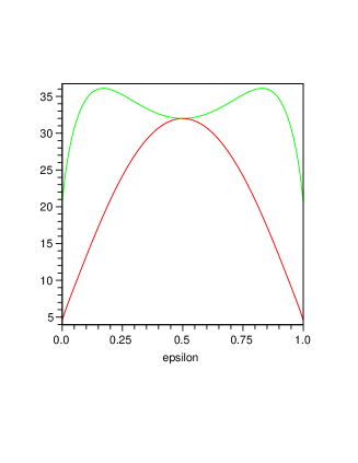
Figure 1: Hyperdistribution $f_{\beta,h}(\epsilon)$ of the mean-field model with $J=1$, $N=5$, $h=0$, and $\beta=0.6$ and $\beta=1.2$, respectively.

Consider spin variables $\sigma_{1},\sigma_{2},\cdots,\sigma_{n}$, taking on values $\pm 1$. The equilibrium states of the ideal paramagnet are the product states

$$q_{\epsilon}(\sigma)=\prod_{n=1}^{N}\epsilon^{\frac{1}{2}(1+\sigma_{n})}(1-\epsilon)^{\frac{1}{2}(1-\sigma_{n})},$$ (9)

with $0\leq\epsilon\leq 1$. The total magnetisation is $\displaystyle\langle M\rangle_{\epsilon}=N(2\epsilon-1)$. The entropy is

$$\check{S}(\epsilon)=-N\epsilon\ln\epsilon-N(1-\epsilon)\ln(1-\epsilon).$$ (10)

Here, we use $\epsilon$ as a parameter instead of $\beta$. Introduce the ferromagnetic Hamiltonian

$$H=-\frac{1}{2}\sum_{m,n=1}^{N}J_{m,n}\sigma_{m}\sigma_{n}-h\sum_{m=1}^{N}\sigma_{m}.$$ (11)

Its average, using the equilibrium distribution of the paramagnet and assuming $J_{mm}=0$, equals $\langle H\rangle_{\epsilon}=-\frac{1}{2}NJ(2\epsilon-1)^{2}-hN(2\epsilon-1)$, with

$$J=\frac{1}{N}\sum_{m,n=1}^{N}J_{m,n}.$$ (12)

The optimised hyperdistribution with parameters $\beta$ (instead of $\theta$) and $h$ is

$$f_{\beta,h}(\epsilon)=\frac{1}{Z(\beta,h)}\exp\left(\check{S}(\epsilon)-\beta\langle H\rangle_{\epsilon}\right)$$ (13)

$$= \frac{1}{Z(\beta,h)}\exp\bigg{(}N\bigg{[}-\epsilon\ln\epsilon-(1-\epsilon)\ln(1-\epsilon)+\frac{1}{2}\beta J(2\epsilon-1)^{2}+\beta h(2\epsilon-1)\bigg{]}\bigg{)}.$$ (14)

For $\beta>\beta_{\rm mf}=J^{-1}$ and $h=0$ the hyperdistribution has two maxima, corresponding to two equally likely states. See the Figure 1. At high temperature the paramagnetic state $q_{\epsilon}(\sigma)$ with $\epsilon=1/2$ is the most likely state. At low temperature the two states with $\epsilon\not=1/2$, maximising $f_{\beta,h}(\epsilon)$, are the most likely ones. This bifurcation from a paramagnetic state to a pair of ferromagnetic states as a function of the temperature $\beta^{-1}$ involves a spontaneous magnetisation of the system.

In the quantum case the ideal paramagnet is described by a density matrix of the product form $\rho_{\theta}^{\otimes N}$, with

$$\rho_{\theta}=\frac{1}{2}+\sum_{k=1}^{3}\theta_{k}\sigma_{k}.$$ (16)

The $\sigma_{k}$ are the Pauli matrices. The Hamiltonian of the Heisenberg model reads

$$H=-\frac{1}{2}\sum_{m,n=1}^{N}J_{m,n}\sum_{k=1}^{3}\sigma_{mk}\sigma_{nk}-h\sum_{n=1}^{N}\sigma_{n3}.$$ (17)

The matrix $\sigma_{mk}$ is a copy of $\sigma_{k}$ at site $m$. Without restriction, assume $J_{nn}=0$. Then the average energy in the product state is $\langle H\rangle_{\theta}=-NJ|\theta|^{2}+Nh\theta_{3}$, with $J$ as in the classical case. The von Neumann entropy of the product state equals

$$S\left(\rho_{\theta}^{\otimes N}\right) = -\frac{N}{2}(1+|\theta|)\ln\frac{1}{2}(1+|\theta|)-\frac{N}{2}(1-|\theta|)\ln\frac{1}{2}(1-|\theta|).$$ (18)

One can now calculate the hyperdistribution $f_{\beta,h}(\theta)$. Note that this is a classical distribution, not an operator. A maximum is attained when the following three equations are satisfied

$$\frac{1}{2}\frac{\theta_{k}}{|\theta|}\ln\frac{1+|\theta|}{1-|\theta|}=-2\beta J\theta_{k}-h\delta_{k,3},\quad k=1,2,3.$$ (19)

Assuming $h\not=0$, the solution requires $\theta_{2}=\theta_{3}=0$. The third parameter $\theta_{3}$ must be a solution of the usual mean-field equation $\theta_{3}=\tanh(\beta J\theta_{3}+\theta_{3}h)$.

4 The microcanonical ensemble

Following Boltzmann, the probability distribution of the microcanonical ensemble equals

$$q_{E}(x)=\frac{c(x)}{\rho(E)}\delta(E-H(x)),$$ (20)

with the density of states $\rho(E)$ given by $\displaystyle\rho(E)=\int{\rm d}x\,c(x)\delta(E-H(x))$. The Boltzmann entropy is $\displaystyle\check{S}(E)=k_{B}\ln\rho(E)$. The optimised hyperdistribution becomes

$$f_{\theta}(E)=\frac{1}{Z(\theta)}\exp\left(\check{\cal S}(E)-\theta E\right)=\frac{\rho(E)}{Z(\theta)}e^{-\theta E}.$$ (21)

The probability distribution $p_{\theta}(x)$ of the hyperensemble coincides with the canonical Boltzmann-Gibbs distribution

$$p_{\theta}(x) \equiv \int_{0}^{\infty}{\rm d}E\,f_{\theta}(E)q_{E}(x)$$ (22)

$$= \int_{0}^{\infty}{\rm d}E\,\frac{\rho(E)}{Z(\theta)}e^{-\theta E}\frac{c(x)}{\rho(E)}\delta(E-H(x))$$ (23)

$$= \frac{c(x)}{Z(\theta)}e^{-\theta H(x)}.$$ (24)

The parameter $\theta$ is the inverse temperature $\beta$.

Figure 2: Number of configurations of a 2x2 and a 3x3 Ising lattice as a function of energy and magnetisation. On the vertical axis is the number of up spins $m$, on the horizontal axis the number of non-matching neighbour pairs $n$.

As an example, involving a discrete phase space, let us consider the 2-dimensional Ising model on a square lattice of $n\times n$ Ising spins. Count the number of configurations $C(m,n)$ with $m$ spins up and $n$ pairs of unequal nearest neighbours. See the Figure 2. The entropy is $\displaystyle\check{\cal S}(m,n)=\ln C(m,n)$. The hyperdistribution is

$$f_{\beta,h}(m,n)=\frac{C(m,n)}{Z(\beta,h)}\exp\left(2\beta J(N-n)-\beta h(N-2m)\right).$$ (25)

At constant $n$ and $h=0$ it is proportional to $C(m,n)$. See the Figure 3. It shows two maxima, corresponding with the spin up and spin down phases.

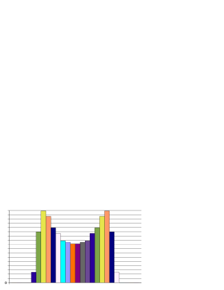
Figure 3: Normalised $C(m,n)$ as a function of $m$ at constant $n=16$ for a 5x5 Ising lattice.

5 Discussion

The aim of the paper is to show that the concept of hyperensembles, as introduced by Crooks CGE07 in a context of non-equilibrium systems, fits well into the standard theory of equilibrium statistical physics. Several situations have been considered. In the example of the ideal gas the hyperensemble approach coincides with the superstatistical treatment of TH04 ; TB05 . In the mean-field theory one starts from a simple model, such as the ideal paramagnet, to solve more complex models under the constraint that the state of the system is an equilibrium state of the simple model. The present formulation in terms of hyperensembles is a mere reformulation of what is known since long. However, it can be applied in a very general context. Such an application beyond the traditional scope of mean-field theory can be found in VdSN06 , where a random walk model is used to model polymer behaviour. In the microcanonical ensemble the probability distribution of the hyperensemble coincides with the canonical Boltzmann-Gibbs distribution. The maximum of the hyperdistribution may be degenerate. This is for instance the case in finite spin lattices with ferromagnetic Ising interaction. Hence, the most-likely microcanonical state is non-unique. Such a feature also occurs in mean-filed models and may be interpreted as a precursor of the phase transition occurring in the thermodynamic limit.

References

- (1) C. Beck and E.G.D. Cohen, Superstatistics, Physica A 322, 267 – 275 (2003).
- (2) C. Beck, Superstatistics: Theoretical concepts and physical applications, to appear in Anomalous transport: Foundations and Applications, ed. R. Klages et al. (Wiley, 2007), arXiv:0705.3832.
- (3) G.E. Crooks, Beyond Boltzmann-Gibbs statistics: Maximum entropy hyperensembles out-of-equilibrium, Phys. Rev. E 75, 041119 (2007), arXiv:cond-mat/0603120.
- (4) H. Touchette, Temperature fluctuations and mixtures of equilibrium states in the canonical ensemble, in Nonextensive Entropy, ed. M. Gell-Mann and C. Tsallis (Oxford University Press, 2004), pp. 159 – 176.
- (5) H. Touchette and C. Beck, Asymptotics of superstatistics, Phys. Rev. E 71, 016131 (2005).
- (6) E. Van der Straeten and J. Naudts, The globule-coil transition in a mean field approach, arXiv:cond-mat/0612256.