A wildland fire model with data assimilation

Abstract

A wildfire model is formulated based on balance equations for energy and fuel, where the fuel loss due to combustion corresponds to the fuel reaction rate. The resulting coupled partial differential equations have coefficients that can be approximated from prior measurements of wildfires. An ensemble Kalman filter technique with regularization is then used to assimilate temperatures measured at selected points into running wildfire simulations. The assimilation technique is able to modify the simulations to track the measurements correctly even if the simulations were started with an erroneous ignition location that is quite far away from the correct one.

, , , , , , and

1 Introduction

Modeling forest fires is a multi-scale multi-physics problem. One can try to account for the many physical processes involved at the appropriate scales, but at the cost of speed. Simplifying appropriate physical processes is one way to obtain a faster-running model. In this paper we also propose using a data assimilation technique to incorporate data in real time. The purpose of this paper is a demonstration-of-concept: we take a very simple model, develop a data assimilation technique, and show how, even with this very simple model, realistic results can be obtained even with significant errors in the initial conditions (location of the fire). This is the first step of a longer-term goal in which a more realistic model will be used.

Data assimilation is a technique used to incorporate data into a running model using sequential statistical estimation. Data assimilation is made necessary by the facts that no model is perfect, the available data is spread over time and space, and it is burdened with errors. The model solution is just one realization from a probability distribution. Data assimilation methods have achieved good success in fields like oil and gas pipeline models [29] and atmospheric, climate, and ocean modeling [52], and they are a part of virtually any navigation system, from steering the Apollo moon spaceships in the 60’s to GPS and operating unmanned drones or rovers in hostile conditions like Afghanistan or Mars today. Data assimilation can also dynamically steer the measurement process, by suggesting locations where the collection of data would result in the best reduction of uncertainty in the forecast [52].

A new paradigm in modeling beyond current techniques in data assimilation is to use Dynamic Data-Driven Application System (DDDAS) techniques [23]. Data assimilation is just one of the techniques from the DDDAS toolbox, which entails the ability to dynamically incorporate additional data into an executing application, and in reverse, the ability of an application to dynamically steer the measurement process. Other DDDAS techniques include deterministic methods such as time rollback, checkpointing, data flow computations, and optimization. One aspect of DDDAS is using data assimilation and measurement steering techniques from weather forecasting in other fields. In a DDDAS, simulations and measurements become a symbiotic feedback control system. Such capabilities promise more accurate analysis and prediction, more precise controls, and more reliable outcomes.

Our ultimate objective is to build a real-time coupled atmospheric-wildland fire modeling system based on DDDAS techniques that is steered dynamically by data, where data includes atmospheric, fire, fuel, terrain, and other data that influence the growth of fires [25, 62, 63, 64]. This work describes one stage of our investigation, that is, to develop and validate techniques to ingest fire data that might originate from in situ and remote sensors into a newly developed fire model. The purpose of this paper is to combine a data assimilation method with a partial differential equation (PDE) based model for wildland fire that achieves good physical behavior and can run faster than real time. The model in this paper does not yet include coupling with the atmosphere, though it is known that such coupling is essential for the wildland fire behavior [20]. Coupling the fire model with atmospheric dynamics as well as with data assimilation is currently under development. Models using explicit, detailed combustion physics are not feasible for prediction, since they require a large number of chemical reactions and species and extremely high resolution (grid cells $<<1m$) fluid dynamics [100]. The actual interaction between the atmosphere and the fire and vegetation is quite complicated, involving turbulence in the vegetation layer and its consequences on heat transfer and combustion [9]. The example provided in this paper is for $250\times 250$ cells of $2m$ size each. A model like FIRETEC [58, 59] could do the same, but including the full interaction between fire, vegetation, and the atmosphere, and it would come at a much higher computational cost. FIRETEC is an example of a physically-based model that simplifies parts of the physics (coarser description than in [100]), but includes the essence of atmosphere-fire interaction. Future developments of the numerics and parallelization of our model are expected to be able to handle realistic fires of the size of several $km$, coupling with the atmosphere, and assimilation of real-time data.

An important point is that our paradigm attempts to strike a balance between model complexity and fast execution. Thus, the present model is based on just two PDEs in two horizontal spatial dimensions: prognostic (predictive) equations for heat and fuel. We use a single semi-empirical reaction rate to achieve the desired combustion model results. In other words, we solve the set of equations known as the reaction-convection-diffusion problem using reaction rates based on the Arrhenius equation, which relates the rate at which a chemical reaction proceeds to the temperature.

This is the simplest combustion model and it is known to produce solutions with traveling combustion waves, that is, a propagating area of localized combustion made up of the preheated area ahead of the fire, the combustion zone, and the post-frontal burning region. One reason for considering a PDE-based model is that even simple reaction-diffusion equations are capable of the complex nonlinear, unsteady behavior such as pulsation and bifurcation that is seen in reality but cannot be reproduced by empirical models.

The characteristics of the combustion wave (maximal temperature, width of the burning region as defined by the leading and trailing edge, and the speed of propagation) are used to calibrate the parameters of the model. We note that physical behavior can be achieved by a very simple model that can reproduce realistic fire behavior very quickly on today’s computers. The PDE-based models in this paper are not necessarily original, cf., e.g., [96], and some PDE coefficients have been determined empirically from measured time-temperature curves before [10, 42, 69], though not in a reaction-diffusion PDE model like the model here. We provide a new systematic procedure for the calibration of the PDE model on real wildland fire data based on separation of nondimensional properties and solution scales. The general calibration problem is an interesting optimal control and stochastic parameter estimation problem in its own right that will be studied in detail in future works.

We then proceed to data assimilation to modify the state of the running model from data. A version of the ensemble Kalman filter (EnKF) is used. This work appears to be the first wildland fire model with data assimilation.

Future extensions of this work include coupling with a numerical weather prediction model, modeling of water content in the fuel, multiple fuel layers, separate treatment of the gas phase (i.e. pyrolysis), crown fire, modeling spotting by stochastic differential equations, preheating by long-range radiation, and contemporary numerical methods such as finite elements and level set methods. The exact number of data points (in space and time) that are necessary for recovering good predictions when the numerical solution diverges from reality depends on the particular data assimilation method used. For the method in this paper, the correction in the location of the fireline should not be larger than the width of the reaction zone. This is similar to the situation for data assimilation into hurricane models, where the correction in the location of the vortex should not be larger than the vortex size [18]. Advanced data assimilation methods that allow sparser data and larger correction are the subject of further research. While real-time data are routinely available for weather forecasting systems, in a wildland fire the data collection is less straightforward. Available data include multi-spectrum infrared airborne photographs, processed to recover the fire region and to some extent the temperature, and radioed data streams from hardened sensors put in the fire path [54, 73, 74]. For overviews of the whole project including computer science aspects, data collection, and visualization, see [64, 63, 62] and [25].

The remainder of the paper is organized as follows. In Section 2, we state our PDE-based fire model. Then in Section 3, we describe the relation of our model to other models in the literature. In Section 4, the model is derived from physical principles in more detail. In Section 5, we develop a method to determine the coefficients of the PDE model using wildland fire data. In Section 6, we describe the ensemble Kalman filter techniques for the data assimilation. In Section 7, we test the PDE and ensemble Kalman filter methods on a two-dimensional representation of a wildland fire and calibrate the models against real data. Finally, Section 8 contains our conclusions.

2 Formulation of the model

We consider the model of fire in a layer just above the ground. First, we define the following terms:

$T$ ($K$) is the temperature of the fire layer,

$S\in\left[0,1\right]$ is the fuel supply mass fraction (the relative amount of fuel remaining),

$k$ ($m^{2}s^{-1}$) is the thermal diffusivity,

$A$ ($Ks^{-1}$) is the temperature rise per second at the maximum burning rate with full initial fuel load and no cooling present,

$B$ ($K$) is the proportionality coefficient in the modified Arrhenius law,

$C$ ($K^{-1}$) is the scaled coefficient of the heat transfer to the environment,   

$C_{S}$ ($s^{-1}$) is the fuel relative disappearance rate,

$T_{a}$ ($K$) is the ambient temperature, and

$\overrightarrow{v}$ ($ms^{-1}$) is the wind speed given by atmospheric data or model.

The model is derived from the conservation of energy, balance of fuel supply, and the fuel reaction rate:

$$\frac{dT}{dt} =\nabla\cdot\left(k\nabla T\right)-\overrightarrow{v}\cdot\nabla T+A\left(Se^{-B/(T-T_{a})}-C\left(T-T_{a}\right)\right),$$ (1)

$$\frac{dS}{dt} =-C_{S}Se^{-B/(T-T_{a})},\quad T>T_{a},$$ (2)

with the initial values

$$S\left(t_{\text{init}}\right)=1\text{ and }T\left(t_{\text{init}}\right)=T_{\text{init}}\text{.}$$ (3)

The diffusion term $\nabla\cdot\left(k\nabla T\right)$ models short-range heat transfer by radiation in a semi-permeable medium, $\overrightarrow{v}\cdot\nabla T$ models heat advected by the wind, $Se^{-B/(T-T_{0})}$ is the rate fuel is consumed due to burning, and $AC\left(T-T_{a}\right)$ models the convective heat lost to the atmosphere. The reaction rate $e^{-B/(T-T_{a})}$ is obtained by modifying the reaction rate $e^{-B/T}$ from the Arrhenius law by an offset to force zero reaction at ambient temperature, with the resulting reaction rate smoothly dependent on temperature.

A more detailed derivation of the model from physical principles is contained in Section 4. Calibration of the coefficients from physically observable quantities will be described in Section 5.

3 Relation to other models

Recent surveys of wildland fire models and their histories are in [70, 75, 85].

3.1 Models based on diffusion-reaction PDEs

It is known that systems of the form (1-2) admit traveling wave solutions. The temperature in the traveling wave has a sharp leading edge, followed by an exponentially decaying cool-down trailing edge. This was observed numerically but we were not able to find a rigorous proof in the literature in exactly this case, though proofs for some related systems exist.

For a related system with fuel diffusion, the existence and speed of traveling waves were obtained by asymptotic methods already in classical work, summarized in the monograph [98]. For the system (1-2), [96] obtains approximate combustion wave speed by heuristic asymptotic methods under the assumption that no heat is lost and ambient temperature is absolute zero, which is equivalent to our setting $C=0$. Models that do not guarantee zero combustion at ambient temperature suffer from the “cold boundary difficulty”: by the time a combustion wave gets to a given location, the fuel at that location is depleted by the ongoing reaction at ambient temperature. So, no perpetual traveling combustion waves can exist, and there are only “pseudo-waves” that travel only for a finite time [13, 67, 98]. [15] derives the speed of traveling waves in a simplified model with the reaction started by ignition at a given temperature, followed by an assumed temperature indepentent reaction rate that is only proportional to the fuel remaining. This is similar to the model in [10].

Equation (1) without fuel depletion (i.e., with constant $S$) and without wind (i.e., $\overrightarrow{v}=0$) is a special case of the nonlinear reaction-diffusion equation,

$$\frac{dT}{dt}=\nabla\cdot\left(\nabla T\right)+f\left(T\right).$$ (4)

Reaction-diffusion equations of the form of equation (4) are known to possess traveling wave solutions, which switch between values close to stationary states given by $f\left(T\right)=0$ [41, 49]. The simplest model problem is Fisher’s equation with $f\left(T\right)=T\left(1-T\right)$, for which the existence of a traveling wave solution and a formula for its speed were proven in [53]. For an analytical study of the evolution of waves to a traveling waveform, see [87], and for a numerical study, see [40, 99]. [80, Ch. 8 and 11] gives proofs of the existence of solution and attractors for reaction-diffusion equations, but does not mention traveling waves. [7] proves the existence of a solution, but not traveling waves, for the reaction-diffusion equation (1) except with a nonlinear diffusion term $\nabla\cdot\left(kT^{3}\nabla T\right)$ and again without considering fuel depletion.

[85] considers a two reaction model (solid and pyrolysis gas), and argues that the modeling of pyrolysis by a separate reaction is essential for capturing realistic fire behavior. For a more complicated model of this type that includes other components, e.g., water vapor, see [43].

Various aspects of special cases of equations (1-2) have been studied in a number of papers. [95] uses a formal expansion in an Arrhenius reaction model to get the wave speed and a prediction of whether a small fire will or will not spread. [65] computes the ignition wave speed and extinction wave speed numerically. The speed and stability of combustion waves are analyzed by asymptotic expansion in [45]. An approximation to the temperature reaction equation gives the size of the reaction zone and the slope of the temperature curve. [71, 72] derive a nonlinear eigenvalue problem for a traveling wave in a different combustion problem, with fuel reaction, solve it numerically by the shooting method, and study the existence and stability of the traveling wave solution. See also [45, 46] for the gas case (i.e., also with fuel diffusion instead of just temperature diffusion).

Enriched finite element methods for the linear diffusion-advection-reaction problem are designed and error estimates given in [8, 22, 36, 37]. However, in all those works, the reaction function $f$ is replaced by a linear function, so there are no traveling wave solutions, and fuel consumption is not considered. [68] compares several time discretization techniques in the presence of nonlinear reaction terms. [6, 34] provide error estimates for mixed finite elements applied to the single species combustion equation and more general reaction-diffusion problems, but again without a fuel balance equation. [84] proposes a nonlinear Galerkin method for reaction-diffusion problems, and proves convergence by a compactness argument. Even simple nonlinear models exhibit bifurcations, which can be examined by direct simulation [90]. Approximation of Fisher’s equation by finite elements are studied numerically in [16, 81], especially regarding the correct wave speed, but no error estimates are given. For finite differences applied to a reaction-diffusion equation, see [57]. Since the common feature of the solutions of reaction-diffusion equations is the development of a sharp wave, with the solution being almost constant elsewhere, interface tracking techniques such as level set methods [86, 89] are relevant here as well.

3.2 Fireline evolution, fire spread, and empirical models

The reaction zone in reaction-diffusion models is typically very thin, and resolving it correctly requires very fine meshes. Hence, a number of models consider the evolution of the fireline instead. Combustion equations in the reaction sheet limit or large activation energy asymptotics reduce to a representation of the reaction zone (here, the fireline) as an evolving internal interface [17, 21, 24, 35, 56, 77], though this reduction does not seem to have been done for exactly the same equations as here. The asymptotic models typically compute the speed of the movement of the reaction interface in the normal direction, often involving its curvature.

Fireline evolution models often postulate empirically observed properties of the fire, such as the fire spread rate in the normal direction, instead of physically based differential equations. Modeling of fireline evolution was reviewed by [94]. [2, 3, 38] derive fire spread rates without using reaction kinetics. [78, 79] study evolution of the fireline as a curve. [27] introduces a convective term in a radiation based model in an attempt to better describe slope effects on rate of spread.

Far fewer examples exist where data was used to calibrate models. Fire spread models based on radiation like [1] are tested against data in [26]. [2, 3] calibrate a mass loss model by crib burning experiments. [82] formulate a model for surface fire spread rate with a physically based core rate of spread in zero wind on flat ground, calibrated to other wind speed and slopes using laboratory measurements. [10] use the energy balance equation coupled with a model of ignition at a threshold temperature, followed by exponential decay. Measured temperature profiles are used to identify parameters of the model. [69, 88] use laboratory data to validate predictions made with different systems of PDEs. [97] use actual fire spread data and theoretical calculations to test the effect of fire front width on surface spread rates through radiative transfer terms. [93] postulates empirical rates of fire spread and of the wind created by the fire and identifies the coefficients from experiments. The feedback between the fire and the surrounding flow is then modeled by a simple one-dimensional differential equation, which is sufficient to explain the conditions for the fire spread to stop or accelerate to a blowup.

3.3 Coupled fluid-fire models

Wildland fire models (either empirical, semi-empirical, or PDE-based) have been coupled to a fluid environment that may be (for small domains) a computational fluid dynamics model (i.e., models the flow and thermodynamics of air) or a numerical weather prediction model (i.e., a computational fluid dynamics model that also considers moist atmospheric processes, the formation of precipitation, and flow over topography).

The FIRETEC model [58, 59] simulates wildland fires by representing the average reaction rates and transport over a resolved volume, usually on the order of $1m^{3}$ in three dimensional space. This attempts to resolve the effects of heat transfer processes without representing each in detail. The ambient environment is air, but the model omits weather processes. [55] gives a multiphase, reactive, and radiative one dimensional model specialized for wildland fires. [28] adds detailed fluid modeling to the model from [55] to study crown fires in air, again with no weather processes and in two dimensions. [44] presents a complicated model of surface and canopy fire based on fluid dynamics and chemical reaction equations where prognostic equations are created for gases that have been grouped into reactive combustible gases, non-reactive combustion products, and an oxidizer ($O_{2}$). Methods of this type are standard in combustion modeling. For a flame model with detailed chemistry and physics, see [30].

An alternate approach is adopted in [19, 20], where a semi-empirical fire spread model based upon the [82] fire spread equation and a canopy fire model are coupled to a numerical weather prediction model to model the interactions between wildland fires and the atmospheric environment. Here, weather processes ranging from synoptic to boundary layer scale are simulated with good fidelity, and the combustion processes are represented by semi-empirical formulas in order to capture the sensible (temperature) and latent (water vapor) heat fluxes into the environment.

4 Derivation of the model

We consider fire in a ground layer of some unspecified finite small thickness $h$. The fire layer consists of the fuel and air just above the fuel. All modeled quantities are treated as two dimensional, homogenized in the vertical direction over the ground layer. We will not attempt to derive equations and substitute coefficients from material properties because of the degree of simplification and uncertainty present in the homogenization. Instead, physical laws will be used to derive the form of the equations and the coefficients will be identified later from the dynamical behavior of the solution. We first derive the system of PDEs based on conservation of energy and fuel reaction rate in Section 4.1 and then discuss the choice of the reaction term in Section 4.2.

4.1 Heat and fuel supply balance equations

The chemical reactions are a heat source. Heat transfer is due to radiation and convection to the atmosphere. The short-range heat transfer due to radiation and turbulence is modeled by diffusion. The two dimensional heat flux through a segment per length unit then is

$$\overrightarrow{q}_{r}=-k_{1}\nabla T\quad(Wm^{-1}).$$ (5)

The constant $k_{1}$ ($WK^{-1}$) will be identified later.

Heat is generated by the chemical reaction of burning. We model the burning as a reaction in which the rate depends on temperature only, so the reaction rate is $C_{S}r\left(T\right)$, where $C_{S}$ is a coefficient of proportionality ($1/s$), and $r$ is dimensionless. Let $F>0$ ($kg\,m^{-2}$) be the concentration of fuel remaining. Then the rate at which the fuel is lost is proportional to the rate of reaction and the amount of fuel available,

$$\frac{dF}{dt}=-FC_{S}r\left(T\right).$$ (6)

The heat generated per unit surface area is then proportional to the fuel lost,

$$q_{g}=A_{1}FC_{S}r\left(T\right),\quad(Wm^{-2})$$ (7)

where $A_{1}$ ($J\;kg^{-1}$) is the heat released per unit mass of fuel.

Heat per unit area lost due to natural convection to the atmosphere due to buoyancy is given by Newton’s law of cooling,

$$q_{c}=C_{a}(T-T_{a}),\quad\left(Wm^{-2}\right)$$ (8)

where $T_{a}$ is the ambient temperature ($K$) and $C_{a}$ ($Wm^{-2}K^{-1}$) is the heat transfer coefficient. In this model, it is assumed that the convective heat transfer is dominant, and so the effect of radiation into the atmosphere is included in (8).

The material time derivative of the temperature is given by

$$\frac{DT}{Dt}=\frac{dT}{dt}+\overrightarrow{v}\cdot\nabla T.$$ (9)

$dT/dt$ is the Eulerian (or spatial) time derivative of temperature, $\overrightarrow{v}$ is the (homogenized) velocity of the air, $\rho$ is the homogenized surface density of the fire layer ($kg\;m^{-3}$), and $c_{p}$ is the homogenized specific heat of the fire layer ($J\,kg^{-1}K^{-1}$). Again, none of the coefficients $h$, $\rho$, or $c_{p}$ can be assumed to be actually known. The units of the product $h\rho c_{p}$ are $JK^{-1}m^{-2}$.

From the divergence theorem, we now obtain the conservation of energy in the fire layer as

$$h\rho c_{p}\frac{DT}{Dt}=\nabla\cdot\overrightarrow{q}_{r}+q_{g}-q_{c}.$$ (10)

The velocity vector $\overrightarrow{v}$ is obtained from the state of the atmosphere as data, or in future work by coupling with an atmospheric model. In the present model, the velocity vector also incorporates the effect of slope: adding to the wind a small multiple of the surface gradient somewhat simulates the effect that fire spreads more readily uphill. In addition, since the speed of the air is zero at the ground level if as usual no-slip conditions are assumed, the homogenized speed through the fire layer should be approximated by scaling the given wind velocity by a constant less than one.

We now write the equations in a form suitable for identification of the coefficients (which will be formally done in Sec. 5). The goal is to obtain a system of equations with a minimal number of coefficients in as simple form as possible. In addition, we wish to relate the coefficients to the behavior of the solution for certain particular coefficient values, rather than to material and physical properties of the medium, which are in general unknown. We introduce the mass fraction of fuel by

$$S=\frac{F}{F_{0}},$$

where $F_{0}$ is the initial fuel quantity. Substituting in the appropriate values for the heat sources and fluxes, (5), (7), and (8), into (9) and (10), and some simple algebra, we obtain the energy balance and fuel reaction rate equations

$$\frac{dT}{dt} =\nabla\cdot\left(k\nabla T\right)-\overrightarrow{v}\cdot\nabla T+A\left(Sr\left(T\right)-C_{0}\left(T-T_{a}\right)\right),$$ (11)

$$\frac{dS}{dt} =-C_{S}Sr\left(T\right),$$ (12)

with

$$k=k_{1}/(h\rho c_{p}),\quad A=A_{1}C_{S}/(hc_{p}\rho),\quad\mbox{and}\quad C_{0}=C_{a}/A_{1}.$$

Alternatively, we could have taken disappearance of fuel on the left hand side of the heat balance equation (10) (fuel that has burned does not need to be heated), which would lead to an equation of the form

$$\left(1+C_{1}S\right)\frac{dT}{dt}=\nabla\cdot\left(k\nabla T\right)+\overrightarrow{v}\cdot\nabla T+A\left(Sr\left(T\right)-C_{0}\left(T-T_{a}\right)\right)$$

instead of (11). We have chosen not to do so since our goal is to work with the simplest possible model, whose coefficients can be identified. The fuel disappearance in the heat equation affects the temperature profile significantly only in the reaction zone, which is the highest part of the temperature curve. Before the ignition, there is a full fuel load, $S=1$, and after a fairly short reaction time, well before most of the cooling takes place, the remaining fuel settles to some residual value which then remains constant. The effect of the decreased heat capacity of the remaining fuel is then absorbed into the cooling term $AC_{0}$.

4.2 Reaction rate

The Arrhenius reaction rate from physical chemistry is given by

$$r\left(T\right)=e^{-B/T},$$ (13)

where the coefficient $B$ has units $K$. This equation is valid only for gas fuel premixed with a sufficient supply of oxygen. This approximation ignores fuel surface effects but it is widely used nonetheless. One consequence of (13) is that the reaction has a nonzero rate at any temperature above absolute zero. Since the time scale for burning is much smaller than the oxidation rate at ambient temperature, we modify (13) so that no oxidation occurs below some fixed temperature, $T_{0}$ (see Section 5), and take instead

$$r\left(T\right)=\left\{\begin{array}[c]{c}e^{-B/\left(T-T_{0}\right)},\quad T>T_{0},\\ 0,\quad T\leq T_{0}.\end{array}\right.$$ (14)

Note that the fuel consumption rate is a smooth function of $T$, which is favorable for a numerical solution, unlike in [7], where a cutoff function was used.

5 Identification of coefficients

We wish to use an observed behavior of the fire rather than physical material properties to identify the coefficients. It is not simple to obtain reasonable behavior of the solution from substituting physical coefficients into the equations. Further, as explained in Section 4, because of a number of simplifying assumptions employed and because of the homogenization of coefficients over a fire layer of unspecified thickness, it is not quite clear what the material properties should be anyway.

We first use basic reaction dynamics and a reduced model to find rough approximate values of the coefficients that produce a reasonable solution. Then we transform the equations to a nondimensional form, which allows us to separate the coefficients into those that determine the qualitative behavior of the solution and those that determine the scales. We propose to use the approximate coefficients obtained from the reduced models as initial values for identification of the coefficients by the nondimensionalization method to match observed temperature profiles.

5.1 Reaction rate coefficients

Consider first the hypothetical case in which $T$ is constant in space, so that only heat due to the reaction (burning) and natural convection contribute non-zero terms in the heat equation, (1), and essentially the full initial fuel supply $F_{0}$ is present at all times (the rate of fuel consumption is negligible, $C_{S}\approx 0$, so $S\approx 1$):

$$\frac{dT}{dt}=A\left(e^{-B/\left(T-T_{0}\right)}-C\left(T-T_{a}\right)\right).$$ (15)

Constant values of temperature which are solutions to (15) are called equilibrium points, and at these points the heat produced by the reaction equals the heat lost to the environment,

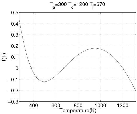
$$f(T)=e^{-B/\left(T-T_{0}\right)}-C\left(T-T_{a}\right)=0.$$ (16)

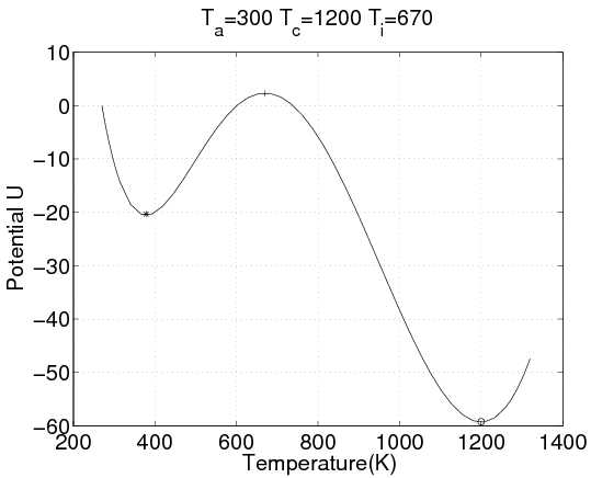
Equation (16) has at most three roots [39], see for example, Figure 1. The first zero, denoted as $T_{p}$, called the lower temperature regime by [39], is a stable equilibrium temperature. If the temperature goes below this temperature then the heat generated from the reaction dominates and the temperature rises. If the temperature goes above this temperature then convective cooling dominates and the temperature decreases. If $T_{0}<T_{a}$, then this point is typically just above the ambient temperature, $T_{a}$, since some reaction is present even at ambient temperature. The middle zero, $T_{i}$, is an unstable equilibrium point. If the temperature goes below $T_{i}$ then convective cooling dominates and the temperature decreases. Above $T_{i}$, the heat due to chemical reactions dominate and the temperature increases. We refer to $T_{i}$ as the auto-ignition temperature, the temperature above which the reaction is self-sustaining [76]. The stable equilibrium at a high temperature, $T_{c}$, is the maximum stable combustion temperature, assuming replenishing of the supply of fuel and oxygen. The temperature $T_{c}$ is called the high temperature regime by [39]. The stability properties of the equilibrium points are also clear from the graph of the potential $U(T),$ defined by $U^{\prime}(T)=f(T)$. The stable equilibrium points are local minima of the potential, while the autoignition temperature is a local maximum and thus an unstable equilibrium (see Fig. 2).

While the coefficients $B$ and $C/F_{0}$ in (16) are generally unknown, they can be found from the equilibrium temperature points. Suppose that two roots $T_{i}$ and $T_{c}$ of $f(T)$ from (16) are given such that $T_{0}\leq T_{a}<T_{i}<T_{c}$. Then simple algebra gives

$$B=\frac{\ln{\left(\frac{T_{i}-T_{a}}{T_{c}-T_{a}}\right)}}{\frac{1}{T_{c}-T_{0}}-\frac{1}{T_{i}-T_{0}}}\quad\mbox{and}\quad C=\frac{e^{-B/(T_{i}-T_{0})}}{T_{i}-T_{a}}.$$ (17)

It should be noted that the coefficients $B$ and $C$ from (17) result in three equilibrium points only when $T_{i}$ is significantly higher than $T_{a}$. When $T_{i}$ is too close to $T_{a}$, the resulting energy balance equation $f(T)=0$ has only two roots. This, however, does not occur for the values of $T_{a}$, $T_{i}$, and $T_{c}$ of interest.

.

Figure 1: Sample reaction heat balance function $f(T)$ from equation (16)

Figure 2: Reaction heat balance potential $U$

Figure 3: Solution with the Arrhenius reaction rate. Due to nonzero reaction rate at ambient temperature, fuel starts disappearing and thus a propagating combustion wave does not develop. The coefficients are $k=2.1360\times 10^{-1}m^{2}s^{-1}K^{-3}$, $A=1.8793\times 10^{2}Ks^{-1}$, $B=5.5849\times 10^{2}K$, $C=4.8372\times 10^{-5}K^{-1}$, and $C_{S}=1.6250\times 10^{-1}s^{-1}$. $T_{c}=1200K$ and $T_{i}=670K$.

Figure 4: Solution with Arrhenius reaction rate modified by temperature offset $T_{a}$ to force zero reaction rate at ambient temperature. A propagating combustion wave develops. The coefficients are $k=2.1360\times 10^{-1}m^{2}s^{-1}K^{-3}$, $A=1.8793\times 10^{2}Ks^{-1}$, $B=5.5849\times 10^{2}K$, $C=4.8372\times 10^{-5}K^{-1}$, and $C_{S}=1.6250\times 10^{-1}s^{-1}$. $T_{c}=1200K$ and $T_{i}=670K$.

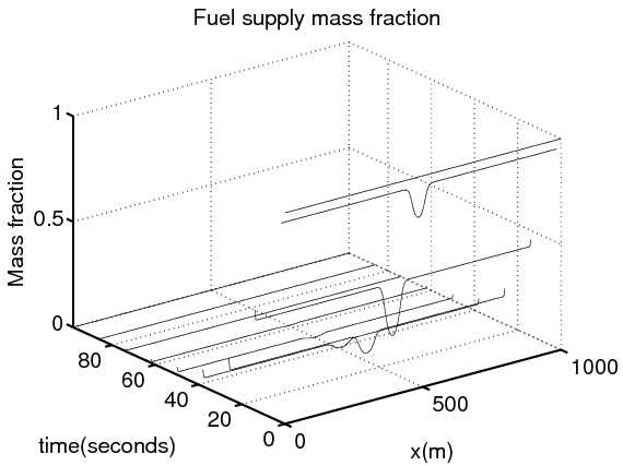
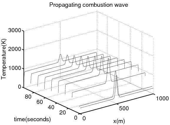
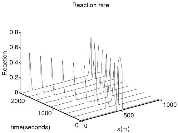
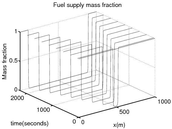
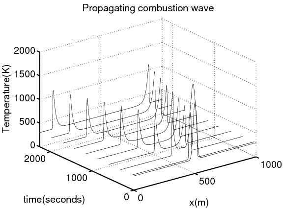
First consider the solution of (11-12) and the reaction rate (14) with $T_{0}=0$. Then the reaction is the Arrhenius rate known from chemistry and there is a nonzero reaction rate at $T=T_{a}$. This results in fuel loss everywhere, and, in our computational experiments, no traveling combustion wave developed (see Fig. 3) since, after a relatively short time, there was not enough fuel to sustain combustion. This phenomenon is known as the cold boundary effect in combustion literature [96]: a traveling combustion wave solution does not exist, and there can only be pseudo-waves that propagate for a limited time [13, 67] and then vanish. Since for the values of $B$ and $C$ obtained from realistic $T_{i}$ and $T_{c}$, the fuel disappears rather quickly, we force the reaction rate, $r(T)$, to be zero at ambient temperature by choosing the offset $T_{0}=T_{a}$. Using the offset by $T_{a}$ is essentially the same as assuming that the ambient temperature is absolute zero as commonly done in combustion literature [96]. In this case, a propagating combustion wave develops (see Figs. 4 and 5). Therefore, we use $T_{0}=T_{a}$.

It should be noted that traveling combustion waves, such as in Fig. 5, are caused by the combined effect of reaction and diffusion; convection does not play a role in this section. The reaction heat diffuses forward on the leading edge, heating the fuel ahead of the wave, until the reaction ahead of the wave can sustain itself, thus causing the combustion to spread. On the trailing edge, the reaction drops off due to fuel depletion, after which temperature decays due to cooling.

5.2 Cooling coefficient

The coefficients $B$ and $C$ in the modified reaction form (16) have been determined from reasonable values of $T_{c}$ and $T_{i}$ by (17). We want to determine the remaining coefficient, $A$. This can be done from the characteristic cooling time. Consider the trailing edge of a traveling combustion wave, after all or most of the fuel has been depleted, temperature drops, and heat generated by the reaction and diffusion drop to an insignificant level. From that point on, the temperature approximately satisfies

$$\frac{dT}{dt}=-AC(T-T_{a}).$$

Thus, at the trailing edge, given $T$ at some time $t_{0}$, we have

$$T(t)=T_{a}+\left(T(t_{0})-T_{a}\right)e^{-AC(t-t_{0})}$$

and we can define the characteristic cooling time, $t_{c}$, to be the time which the fire layer takes to cool by a factor of $1/e$, i.e.,

$$T(t_{0}+t_{c})-T_{a}=\frac{1}{e}\left(T(t_{0})-T_{a}\right),$$

which proves that$ACt_{c}=1$, or

$$A=\frac{1}{Ct_{c}}.$$ (18)

5.3 Scales and non-dimensional coefficients

We now write the model in terms of nondimensional variables, which control the qualitative behavior of the system (1-2). Again, we do not consider the wind here yet, and so

$$\frac{dT}{dt} =\nabla\left(k\nabla T\right)+A\left(Se^{-\frac{B}{T-T_{a}}}-C\left(T-T_{a}\right)\right),$$ (19)

$$\frac{dS}{dt} =-SC_{S}e^{-\frac{B}{T-T_{a}}},\qquad T>T_{a}.$$ (20)

The substitution

$$\widetilde{T}=\frac{T-T_{a}}{B},\qquad\widetilde{x}=\frac{x}{k^{1/2}B^{1/2}A^{-1/2}},\qquad\mbox{and}\qquad\widetilde{t}=\frac{tA}{B}$$

transforms (19-20) into a non-dimensional form

$$\frac{d\widetilde{T}}{d\widetilde{t}} =\widetilde{\nabla}\cdot\left(\widetilde{\nabla}\widetilde{T}\right)+\widetilde{S}e^{-1/\widetilde{T}}-\lambda\widetilde{T},$$ (21)

$$\frac{d\widetilde{S}}{d\widetilde{t}} =-\beta\widetilde{S}e^{-1/\widetilde{T}},\qquad\widetilde{T}>0,$$ (22)

with two dimensionless coefficients

$$\lambda=CB\quad\mbox{and}\quad\beta=\frac{BC_{S}}{A}.$$ (23)

Therefore, the qualitative behavior of the solution is determined only by the nondimensional coefficients $\lambda$ and $\beta$, which can be varied independently.

The nondimensional form (21-22) suggests a strategy for identification of the coefficients $k$, $A$, $B$, $C$, $C_{S}$: first match nondimensional properties of the traveling combustion wave, such as the ratio of the width of the leading edge and the trailing edge and the fuel fraction remaining after the combustion wave by varying $\lambda$ and $\beta$. The width of the wave can be measured e.g. as the distance of the points where the temperature equals 50% of the maximum. The nondimensional traveling wave solution $\widetilde{T}(\widetilde{t},\widetilde{x})$, $\widetilde{S}(\widetilde{t},\widetilde{x})$ has some (nondimensional) maximal temperature $\widetilde{T}_{\max}$, width $\widetilde{w}$, and speed $\widetilde{v}$, while the data (a measured temperature profile) has maximal temperature $T_{\max}$, the width $w$, and the speed $v$ of the traveling wave. This determines the scales

$$T_{1}=\frac{T_{\max}}{\widetilde{T}_{\max}},\quad x_{1}=\frac{w}{\widetilde{w}},\quad\mbox{and}\quad t_{1}=\frac{vw}{\widetilde{v}\widetilde{w}}.$$

By the substitution

$$\widetilde{T}=\frac{T-T_{a}}{T_{1}},\qquad\widetilde{x}=\frac{x}{x_{1}},\qquad\mbox{and}\qquad\widetilde{t}=\frac{t}{t_{1}}$$

into the system (19-20) with the coefficients

$$A=T_{1}/t_{1},\quad B=T_{1},\quad C=\lambda/T_{1},\quad C_{S}=\beta/t_{1},\quad\mbox{and}\quad k=x_{1}^{2}/\left(T_{1}^{3}t_{1}\right)$$ (24)

admits the scaled solution

$$T(t,x)=T_{1}\widetilde{T}\left(\frac{t}{t_{1}},\frac{x}{x_{1}}\right)+T_{a},\quad\mbox{and}\quad S(t,x)=\widetilde{S}\left(\frac{t}{t_{1}},\frac{x}{x_{1}}\right),$$

which has the desired nondimensional properties as well as the correct maximal temperature, width, and speed of a traveling combustion wave.

A dimensionless system similar to (21-22) is studied in [96] in the case $\lambda=0$, i.e., combustion insulated against heat loss. [96] determine the speed of the traveling wave as a function of $\beta$ numerically and by an asymptotic expansion and observe that a traveling combustion wave exists only for small values of $\beta$. By increasing $\beta$, the solution is periodic, then the period doubles, and eventually the solution becomes chaotic. We have observed that increasing $\beta$ has a similar effect for the equations (21-22) when $\lambda>0$. Also, we have observed that a sustained combustion wave is possible only when $\lambda$ is small enough. A systematic study of the properties of (21-22) for various values of $\lambda$ and $\beta$ will be done elsewhere. For a dimensionless system similar to ours, but without the temperature offset to force zero reaction at ambient temperature, see [7].

6 Data Assimilation

The goal in data assimilation on a fire model is a filter that can effectively track the location of the fireline given data in the form of temperature and remaining fuel at sample points inside of the domain. The fire application is particularly troublesome for EnKFs. The standard method for generating an initial ensemble is not sufficient for this scenario. Namely, taking an initial guess at the model state (temperature and fuel) and adding to it a smooth random field. Here, if the data indicates that the fireline has shifted away from that of the ensemble, then the Kalman Filter will generally ignore the data entirely due to the extraordinarily small data likelihood. Clearly, such an initial ensemble does not properly represent the prior uncertainty in the location of the ignition region, only that of the temperature of ignition. In order to represent this uncertainty as well, we have also perturbed the state variables by a spatial shift [50]. However, this approach leads to further potential problems for EnKF. Due to the relatively sharp temperature profile of the fireline, the temperature at each grid point will tend to be close to that of the stable ambient or burning temperatures. A similar situation occurs with the fuel near the fireline as well. This is indicative of a strongly bimodal or non-Gaussian prior distribution. Despite this violation of the underlying assumptions of EnKF, we have found that it is possible to track large changes in the fireline, as shown in the numerical results in Section 7.

The Ensemble Kalman Filter (EnKF) is a Monte-Carlo implementation of the Bayesian update problem: Given a probability distribution of the modeled system (the prior, often called the ‘forecast’ in geophysical sciences) and data likelihood, the Bayes’ theorem is used to obtain the probability distribution with the data likelihood taken into account (the posterior or the ‘analysis’). The Bayesian update is combined with advancing the model in time, with the data incorporated from time to time. The original Kalman Filter [51] relies on the assumption that the probability distributions are Gaussian (‘the Gaussian assumption’), and provides algebraic formulas for the change of the mean and covariance by the Bayesian update, and a formula for advancing the covariance matrix in time provided the system is linear. However, this is not possible computationally for high-dimensional systems. For this reason, EnKFs were developed in [31, 48]. EnKFs represent the distribution of the system state using an ensemble of simulations, and replace the covariance matrix by the covariance matrix of the ensemble. One advantage of EnKFs is that advancing the probability distribution in time is achieved by simply advancing each member of the ensemble. EnKFs, however, still rely on the Gaussian assumption, though they are of course used in practice for nonlinear problems, where the Gaussian assumption is not satisfied. Related filters attempting to relax the Gaussian assumption in EnKF include [5, 11, 12, 61, 92].

We use the EnKF following [14, 32], with only some minor differences. This filter involves randomization of data. For filters without randomization of data, see [4, 33, 91]. The data assimilation uses a collection of independent simulations, called an ensemble. The ensemble filter consists of

1. generating an initial ensemble by random perturbations,

2. advancing each ensemble member in time until the time of the data, which gives the so-called forecast ensemble

3. modifying the ensemble members by injecting the data (the analysis step), which results in the so-called analysis ensemble

4. continuing with step 2 to advance the ensemble in time again.

We now consider the analysis step in more detail. We have the forecast ensemble

$$U^{f}=[u_{1}^{f},\ldots,u_{N}^{f}]=[u_{i}^{f}]$$

where each $u_{i}^{f}$ is a column vector of dimension $n$, which contains the whole simulation state (in our case, the vector of the values of $T$ and $S$ at mesh nodes). Thus, $U^{f}$ is a matrix of dimension $n$ by $N$. The superscript ^f stands for “forecast”. The data is given as a measurement vector $d$ of dimension $m$ and data error covariance matrix $R$ of dimension $m$ by $m$. The correspondence of the data and the simulation states is given by an observation function $h(u)$ that creates synthetic data, that is, what the data would have been if the simulation and the measurements were exact. We assume that $h$ is linear,

$$h\left(u\right)=Hu.$$ (25)

Using the notation that $\propto$ means proportional and $N(x,M)$ represents a normal distribution with mean $x$ and covariance matrix $M$, the observation being assimilated is

$$Hu-d\sim N\left(0,R\right)$$ (26)

for some matrix $H$. The observation function defines the data likelihood (the probability density of $d$ given the state $u$). Assuming the data error is normally distributed, the data likelihood is

$$p\left(d|u\right)\propto e^{-\frac{1}{2}\left(h\left(u\right)-d\right)R^{-1}\left(h\left(u\right)-d\right)}.$$

The forecast ensemble $U^{f}$ is considered a sample from the prior distribution $p(u)$, and the EnKF strives to create an analysis ensemble that is a sample from the posterior distribution $p\left(u|d\right)$, which is the probability distribution of $u$ after the data has been injected. From Bayes’ theorem of probability theory, we have

$$p\left(u|d\right)\propto p\left(d|u\right)p(u),$$ (27)

[32, eq. (20)]. If $p\sim N(u^{f},Q^{f})$, then it is known that the posterior is also normally distributed with mean

$$u^{a}=u^{f}+K\left(d-Hu^{f}\right),$$ (28)

where $K$ is the Kalman gain matrix,

$$K=Q^{f}H^{\mathrm{T}}\left(HQ^{f}H^{\mathrm{T}}+R\right)^{-1}.$$ (29)

The EnKF is based on applying a version of the Kalman update (28) to each forecast ensemble member $u_{i}^{f}$ to yield the analysis ensemble member $u_{i}^{a}$. For this update, the data vector $d$ in (28) is replaced by a randomly perturbed vector

$$d_{j}=d+v_{j},\quad v_{j}\sim N\left(0,R\right).$$ (30)

Let $\bar{u}^{f}$ be the mean of the forecast ensemble,

$$\bar{u}^{f}=\frac{1}{N}\sum_{i=1}^{N}u_{i}^{f}.$$ (31)

The unknown covariance matrix $Q^{f}$ in (29) is replaced by the covariance matrix $C^{f}$ of the forecast ensemble $U^{f}$,

$$C=\frac{1}{N-1}AA^{T},\quad A=[u_{1}^{f}-\bar{u}^{f},\ldots,u_{N}^{f}-\bar{u}^{f}].$$ (32)

Define

$$D=\left[d+v_{1},\ldots,d+v_{N}\right]$$

as the matrix formed from the randomly perturbed data vectors and

$$U^{a}=[u_{1}^{a},\ldots,u_{N}^{a}]=[u_{i}^{a}]$$

as the analysis ensemble. This gives the EnKF formula,

$$U^{a}=U^{f}+CH^{T}\left(HCH^{T}+R\right)^{-1}(D-HU^{f}).$$ (33)

See [32, eq. (20)] for details. The only difference between (33) and [32, eq. (20)] is that we use the covariance matrix $R$ of the measurement error (which is assumed to be known anyway) rather than the sample covariance matrix of the randomized data. Since $R$ is in practice positive definite, there is no difficulty with the inverse in (33). The matrix $R$ is known from (26). In [32, eq. (20)], the sample covariance matrix, called $R_{e}$, of the perturbed data is used in place of $R$. For large $n$, the matrix $R_{e}$ is singular and then a more expensive pseudoinverse using an eigenvalue decomposition [32, eq. (56)] must be used. Alternately, the data perturbations have to be chosen in a special way [32, eq. (57)].

6.1 EnKF implementation

We have used the ensemble update (33) with the inverse computed by an application of the Sherman-Morrison-Woodbury formula [47]

$$\left(HCH^{T}+R\right)^{-1}=\left(R+\frac{1}{N-1}HA\left(HA\right)^{T}\right)^{-1}=$$

$$R^{-1}\left[I-\frac{1}{N-1}\left(HA\right)\left(I+\left(HA\right)^{T}R^{-1}\frac{1}{N-1}\left(HA\right)\right)^{-1}\left(HA\right)^{T}R^{-1}\right].$$ (34)

This formula is advantageous when the data error covariance matrix $R$ is of a special form such that left and right multiplications by $R^{-1}$ can be computed inexpensively. In particular, when the data errors are uncorrelated, which is usually the case in practice and the case here, the matrix $R$ is diagonal. Then the EnkF formula (33) with (34) costs $O\left(N^{3}+mN^{2}+nN^{2}\right)$ operations, which is suitable both for a large number $n$ of the degrees of freedom and a large number $m$ of data points. Also, (33) can be implemented without forming the observation matrix $H$ explicitly by only evaluating the observation function $h$ using

$$\left[HA\right]_{i} =Hu_{i}^{f}-H\frac{1}{N}\sum_{j=1}^{N}u_{i}^{f}=h\left(u_{i}^{f}\right)-\frac{1}{N}\sum_{j=1}^{N}h\left(u_{i}^{f}\right),$$

$$d-Hu_{i}^{f} =d-h\left(u_{i}^{f}\right).$$

See [60] for further details.

The ensemble filter formulas are operations on full matrices, and they were implemented in a distributed parallel environment using MPI and ScaLAPACK. EnKF is naturally parallel: each ensemble member can be advanced in time independently. The linear algebra in the Bayesian update step links the ensemble members together.

6.2 Regularization

EnKF produces the analysis ensemble in the span of the forecast ensemble. This results in nonphysical states especially if the states in the span are far away from the data. For cheap numerical methods and a highly nonlinear problem, EnKF can easily knock the state out of the stability region. In order to ease this problem, we add an independent observation

$$\bigtriangledown u^{a}-\bigtriangledown\bar{u}^{f}\sim N(0,D),$$

where $\bigtriangledown$ is the spatial gradient, computed by finite differences. This is easily implemented by running the EnKF formulas a second time. In practice, this matrix, $D$, is of the form $\rho I$, where $\rho$ is a regularization parameter. This technique prevents large, nonphysical gradients in the analysis ensemble. See [50] for further details.

7 Numerical results

7.1 Calibration of coefficients in one dimension

Figure 5: Temperature profile of traveling wave. The wave moved about 398m from the initial position in 2300s.

Figure 6: Time-temperature profile (dotted line) measured in a grass wildland fire at a fixed sensor location, digitized from [54], and a computed profile (solid line) from simulation.

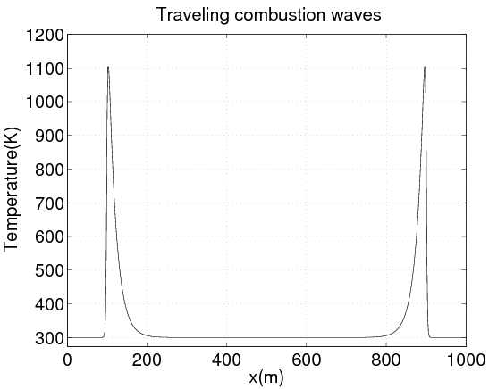
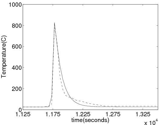
We have found initial values $B=5.5849\times 10^{4}K$, and $C=5.9739\times 10^{-4}K^{-1}$ from the values $T_{i}=670K$ and $T_{c}=1200K$ using (17), and then the value $A=1.5217\times 10^{1}Ks^{-1}$ from (18), using the value $t_{c}=110s$ from [54]. Not every initial condition gives rise to a traveling combustion wave [67]. Inspired by [66], we use an initial condition of the form $T(x,t_{0})=T_{c}e^{-\left(x-x_{0}\right)^{2}/\sigma^{2}}+T_{a}$, where $x_{0}$ is in the center of the interval and $\sigma=10\sqrt{2}m$. This initial condition is smooth. Thus, it does not excite possible numerical artifacts. It has numerically local support and for a modest $\sigma$ provides ignition sufficient to develop into two sustained combustion waves traveling from the center. We have then found empirically suitable values of $k$ and $C_{S}$ that result in traveling combustion waves, computed the nondimensional coefficients $\lambda$ and $\beta$, adjusted them using Fig. 6 (dotted line), and scaled using (24) to match the maximal temperature and the width of the wave in Fig. 6 (dotted line), and the speed of the traveling combustion wave, $0.17m/s$, from [54]. There was a small amount of wind in [54], however we have not considered the wind here. The resulting coefficients are $k=2.1360\times 10^{-1}m^{2}s^{-1}K^{-3}$, $A=1.8793\times 10^{2}Ks^{-1}$, $B=5.5849\times 10^{2}K$, $C=4.8372\times 10^{-5}K^{-1}$, and $C_{S}=1.6250\times 10^{-1}s^{-1}$. The corresponding nondimensional coefficients were $\lambda=2.7000\times 10^{-2}$ and $\beta=0.4829$. The computed traveling combustion wave (see Figs. 4, 5 and 6, solid line) is a reasonable match with the observation (see Fig. 6, dotted line). The trailing edge of the computed temperature profile (see Fig. 6, solid line) was not so well matched but this model is quite limited and other matches reported in the literature are similar [10]. The real data looks like the superposition of two exponential decay modes, possibly the fast one from cooling and the long one from the heat stored in water in the ground.

We have also noted that when the ratio $A/C_{S}$ increases the temperature in the traveling combustion wave increases, increasing the thermal diffusivity coefficient $k$ increases the width and speed of the combustion wave and that the maximum temperature in the traveling wave decreases if $C_{S}$ increases. Sufficiently small value of $C_{S}$ is needed for sustained combustion. We have noted that the numerical solution by finite differences becomes unstable when the ratio $k/h$, where $h$ is the mesh size, is too small.

7.2 Numerical results in two dimensions

We have implemented the fire model in two dimensions by central finite differences in space. The mesh size was $250$ by $250$ and the mesh step was $2m$. We have used the explicit Euler method with time step $1s$. The initial conditions were given by the ambient temperature $T_{a}=300K$ everywhere except in a $50m{\times}50m$ square ignition region which was ignited by elevating the temperature to $1200K$. The mass fraction of the fuel was initialized to be one everywhere except for a $25m$ fuel break in the center of the domain. Then, at each grid point, the fuel was shifted by a random number in $[-0.3,0.3]$. This is intended to simulate a natural uniform fuel supply and a road as a fuel break. The Neumann boundary conditions were specified on all boundaries with no ambient wind across the domain.

The initial ensemble was generated by perturbing the temperature profile of what we call the comparison solution $T_{0}$ utilizing smooth random fields in the following form:

$$\tilde{u}=\sum_{n=1}^{d}\frac{v_{n}}{1+n^{2\alpha}}e_{n},\quad v_{n}\sim N\left(0,1\right),$$ (35)

where $\alpha$ is the order of smoothness of the random field, and $\left\{e_{n}\right\}_{n=1}^{d}$ is the Fourier sine basis, ensuring that $\tilde{u}$ is real valued [31, 83]. This process can be understood as a finite dimensional version of sampling out of normal distribution on an infinite dimensional space of smooth functions, the Sobolev space $H_{0}^{\alpha}\left(\Omega\right)$ [61]. For integer $\alpha$, this is the space of functions with square integrable derivatives of order $\alpha$ and zero traces on the boundary.

A preliminary ensemble was generated by adding a smooth random field to each state variable of the comparison solution. For example, the temperature of $k^{th}$ ensemble member is given by

$$\hat{T}_{k}=T_{0}+c_{T}\tilde{u}_{k},$$ (36)

where the scalar $c_{T}$ controls the magnitude of this perturbation. Finally, the preliminary ensemble was moved spatially in both $x$ and $y$ directions by

$$T_{k}(x,y)=\hat{T}_{k}(x+c_{x}\tilde{u}_{i_{k}}(x,y),y+c_{y}\tilde{u}_{j_{k}}(x,y)).$$ (37)

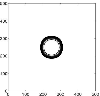
Here, $c_{x}$ and $c_{y}$ control the magnitude of the shift in each coordinate, bilinear interpolation is used to determine $\hat{T}$ on off-grid points, and the temperature outside of the computational domain is assumed to be at the ambient temperature. The given simulation was run with the initialization parameters $c_{T}=5$ and $c_{x}=c_{y}=150$. Fig. 7 shows the effect of these perturbations on a simple circular fire line on the center of the domain.

In each analysis cycle, the solution was advanced by $100s$, and then the data was injected. The data was created artificially by sampling the temperature and fuel of one fixed solution, called the reference solution, every $10m$ (or 5 grid points) across the domain. The data covariance matrix was taken to be diagonal with a variance $10$ for each sample, and the regularization was used with regularization parameter $\rho=750$. The reference solution was created in the same manner as the ensemble with an ignition region located $100m$ away in one direction. This discrepancy is intended to demonstrate the power of EnKF to attract the ensemble to the truth. After each analysis cycle, the ensemble was further perturbed by $5\%$ magnitude of the initial perturbation to assure sufficient ensemble spread for future assimilations.

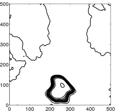
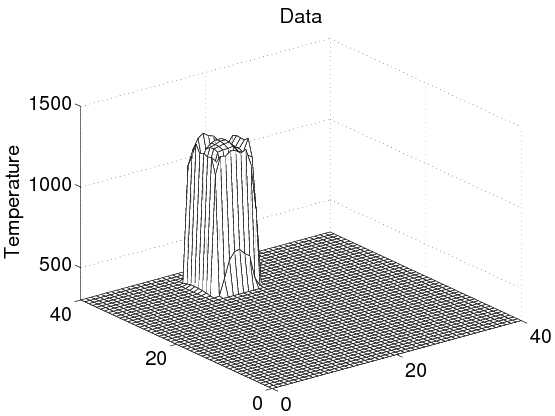
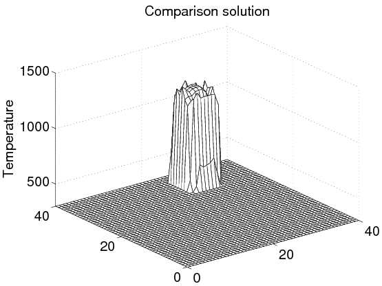
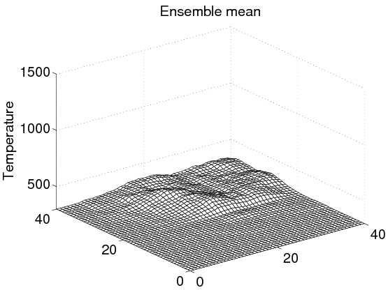
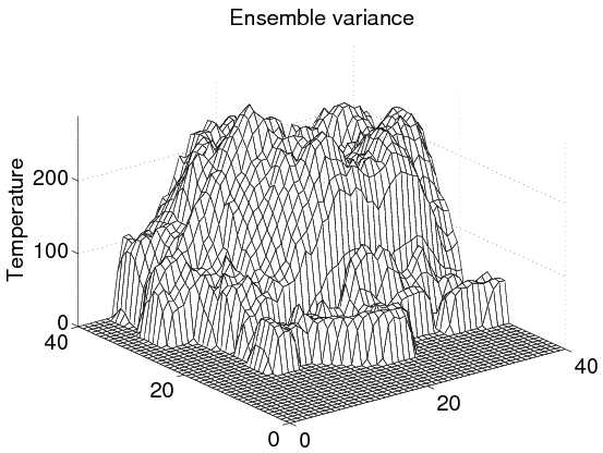
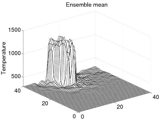
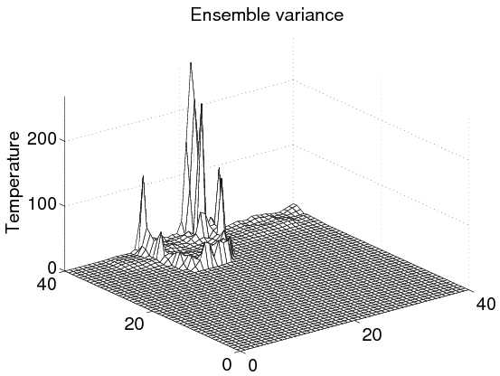
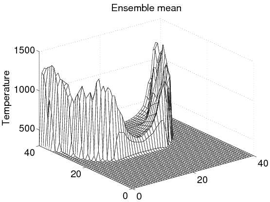
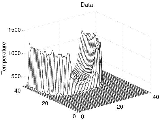
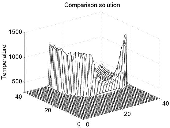
Fig. 8 shows the reference and comparison solution $100s$ after initialization, at the end of the first cycle. Fig. 9 shows the ensemble mean and variance at the same time prior to performing an assimilation. Fig. 10 shows the ensemble after applying the first assimilation. The analysis cycle was repeated $10$ times with the results shown in Figs. 11 and 12. These figures show a remarkable agreement of the ensemble mean with the reference solution, even if the simulation ensemble was ignited intentionally far away from the reference ignition region. However, it should be noted that different runs of this stochastic algorithm produce different results. Sometimes the ensemble is attracted to the reference solution, and sometimes not, depending on if there exists a good match to the data in the span of a fairly small ensemble.

(a)	(b)

Figure 7: Contour plots with $100K$ between contour lines. (a) The temperature profile of a circular ignition region in the center of domain. (b) The same profile randomly perturbed in magnitude by (36) with $c_{T}=5$ and spatially by (37) with $c_{x}=c_{y}=100$.

(a)	(b)

Figure 8: Temperature profiles representing (a) the data (reference solution, taken as the truth) and (b) an unperturbed ensemble member comparison solution $100s$ after initialization.

(a)	(b)

Figure 9: After advancing the solution in time by $100s$ before any data assimilations: Pointwise prior ensemble (a) mean and (b) variance.

(a)	(b)

Figure 10: After advancing the solution in time by $100s$ and performing a single data assimilation: Pointwise posterior ensemble (a) mean and (b) variance.

(a)	(b)

Figure 11: After $10$ analysis cycles with a $100s$ time update per cycle, (a) the ensemble mean compared to (b) the reference solution (the data).

Figure 12: Comparison solution advanced to $1000s$. This is what the solution in Fig. 11 (a) would be without data assimilation.

8 Conclusion

A simple model based on two coupled PDEs can reproduce the time-temperature curve recorded as a wildfire burns over a sensor, which is a measurable feature of fire behavior. By separating the parameters that determine the qualitative properties of the solution from the parameters that determine the temperature, time, and space scales, we were able to identify the parameters of the model from actual wildfire observations. Assimilation of data into a wildfire simulation poses a particular challenge because the combustion region is quite thin. We have shown that a version of the Ensemble Kalman filter is able to assimilate data into a wildfire simulation successfully. The filter uses penalization of nonphysical solution and perturbations by smooth random transformations of the spatial domain, in addition to standard smooth additive perturbation.

9 Acknowledgments

This material is based upon work supported by the National Science Foundation (NSF) under grants CNS-0325314, CNS-0324989, CNS-0324876, CNS-0324910, CNS-0720454, CNS-0719641, CNS-0719626, EIA-0219627, ACI-0305466, OISE-0405349, CNS-0540178, DMS-0610039, and by a National Center for Atmospheric Research (NCAR) Faculty Fellowship. Computer time on IBM BG/L was provided in part by NSF MRI Grants CNS-0421498, CNS-0420873, CNS-0420985, NSF sponsorship of the NCAR, the University of Colorado, and a grant from the IBM Shared University Research (SUR) program. TeraGrid computer time was provided by the NSF through TeraGrid resources at the National Center for Supercomputing Applications, the San Diego Supercomputing Center, the Texas Advanced Computing Center, and the Pittsburgh Supercomputing Center. The authors would like to thank Bob Kremens for suggesting an explanation for the behavior of the measured temperature in Fig. 6. The authors would like to thank an anonymous referee for useful comments that contributed to improving this paper.

References

- [1] F. A. Albini, A model for fire spread in wildland fuels by radiation - A model including fuel cooling by convection, Combustion and Science Technology 45 (1986) 101–113.
- [2] F. A. Albini, PROGRAM BURNUP: A simulation model of the burning of large woody natural fuels, final Report on Research Grant INT-92754-GR by U.S.F.S. to Montana State Univ., Mechanical Engineering Dept. (1994).
- [3] F. A. Albini, E. D. Reinhardt, Improved calibration of a large fuel burnout model, Int. J. Wildland Fire 7 (1997) 21–28.
- [4] J. L. Anderson, An ensemble adjustment Kalman filter for data assimilation, Monthly Weather Review 129 (1999) 2884–2903.
- [5] J. L. Anderson, S. L. Anderson, A Monte Carlo implementation of the nonlinear filtering problem to produce ensemble assimilations and forecasts, Monthly Weather Review 127 (1999) 2741–2758.
- [6] M. I. Asensio, L. Ferragut, Total error estimates of mixed finite element methods for nonlinear reaction-diffusion equations, Neural Parallel Sci. Comput. 8 (2) (2000) 169–189.
- [7] M. I. Asensio, L. Ferragut, On a wildland fire model with radiation, Int. J. Numer. Meth. Engrg. 54 (2002) 137–157.
- [8] M. I. Asensio, A. Russo, G. Sangalli, The residual-free bubble numerical method with quadratic elements, Mathematical Models and Methods in Applied Sciences 14 (5) (2004) 641–661.
- [9] P. G. Baines, Physical mechanisms for the propagation of surface fires, Mathematical and Computer Modelling 13 (1990) 83–94.
- [10] J. H. Balbi, P. A. Santoni, J. L. Dupuy, Dynamic modelling of fire spread across a fuel bed, International J. of Wildland Fire 9 (4) (1999) 275–284.
- [11] J. D. Beezley, J. Mandel, Morphing ensemble Kalman filters, Tellus 60A (2008) 131–140.
- [12] T. Bengtsson, C. Snyder, D. Nychka, Toward a nonlinear ensemble filter for high dimensional systems, Journal of Geophysical Research - Atmospheres 108(D24) (2003) STS 2–1–10.
- [13] H. Berestycki, B. Larrouturou, J.-M. Roquejoffre, Mathematical investigation of the cold boundary difficulty in flame propagation theory, in: P. C. Fife, A. Liñán, F. Williams (eds.), Dynamical issues in combustion theory (Minneapolis, MN, 1989), vol. 35 of IMA Vol. Math. Appl., Springer, New York, 1991, pp. 37–61.
- [14] G. Burgers, P. J. van Leeuwen, G. Evensen, Analysis scheme in the ensemble Kalman filter, Monthly Weather Review 126 (1998) 1719–1724.
- [15] D. Campos, J. E. Llebot, J. Fort, Reaction-diffusion pulses: a combustion model, J. Phys. A: Math. Gen. 37 (2004) 6609–6621.
- [16] G. F. Carey, Y. Shen, Least-squares finite element approximation of Fisher’s reaction-diffusion equation, Numer. Methods Partial Differential Equations 11 (2) (1995) 175–186.
- [17] X. Chen, Generation and propagation of interfaces in reaction-diffusion systems, Trans. Amer. Math. Soc. 334 (2) (1992) 877–913.
- [18] Y. Chen, C. Snyder, Assimilating vortex position with an ensemble Kalman filter, Monthly Weather Review 135 (2007) 1828–1845.
- [19] T. L. Clark, J. Coen, D. Latham, Description of a coupled atmosphere-fire model, Intl. J. Wildland Fire 13 (2004) 49–64.
- [20] T. L. Clark, M. A. Jenkins, J. Coen, D. Packham, A coupled atmospheric-fire model: Convective feedback on fire line dynamics, J. Appl. Meteor 35 (1996) 875–901.
- [21] A. G. Class, B. J. Matkowsky, A. Y. Klimenko, A unified model of flames as gasdynamic discontinuities, J. Fluid Mech. 491 (2003) 11–49.
- [22] R. Codina, Comparison of some finite element methods for solving the diffusion-convection-reaction equation, Comput. Methods Appl. Mech. Engrg. 156 (1-4) (1998) 185–210.
- [23] F. Darema, Dynamic data driven applications systems: A new paradigm for application simulations and measurements, in: M. Bubak, G. D. van Albada, P. M. A. Sloot, J. J. Dongarra (eds.), Computational Science-ICCS 2004: 4th International Conference, vol. 3038 of Lecture Notes in Computer Science, Springer, 2004, pp. 662–669.
- [24] J. W. Dold, R. W. Thatcher, A. A. Shah, High order effects in one step reaction sheet jump conditions for premixed flames, Combust. Theory Model. 7 (1) (2003) 109–127.
- [25] C. C. Douglas, J. D. Beezley, J. Coen, D. Li, W. Li, A. K. Mandel, J. Mandel, G. Qin, A. Vodacek, Demonstrating the validity of a wildfire DDDAS, in: V. N. Alexandrov, D. G. van Albada, P. M. A. Sloot, J. Dongarra (eds.), Computational Science ICCS 2006: 6th International Conference, Reading, UK, May 28-31, 2006, Proceedings, Part III, vol. 3993 of Lecture Notes in Computer Science, Springer, Berlin/Heidelberg, 2006, pp. 522–529.
- [26] J.-L. Dupuy, Testing two radiative physical models for fire spread through porous forest fuel beds, Combustion Science and Technology 155 (1) (2000) 149–180.
- [27] J.-L. Dupuy, M. Larini, Fire spread through a porous forest fuel bed: A radiative and convective model including fire-induced flow effects, International J. of Wildland Fire 9 (3) (1999) 155–172.
- [28] J.-L. Dupuy, D. Morvan, Numerical study of a crown fire spreading toward a fuel break using a multiphase physical model, International Journal of Wildland Fire 14 (2005) 141 –151.
- [29] H. E. Emara-Shabaik, Y. A. Khulief, I. Hussaini, A non-linear multiple-model state estimation scheme for pipeline leak detection and isolation, Proceedings of the Institution of Mechanical Engineers, Part I: Journal of Systems and Control Engineering 216 (2002) 497–512.
- [30] A. Ern, C. C. Douglas, M. D. Smooke, Detailed chemistry modeling of laminar diffusion flames on parallel computers, The International Journal of Supercomputer Applications and High Performance Computing 9 (1995) 167–186.
- [31] G. Evensen, Sequential data assimilation with nonlinear quasi-geostrophic model using Monte Carlo methods to forecast error statistics, Journal of Geophysical Research 99 (C5) (10) (1994) 143–162.
- [32] G. Evensen, The ensemble Kalman filter: Theoretical formulation and practical implementation, Ocean Dynamics 53 (2003) 343–367.
- [33] G. Evensen, Sampling strategies and square root analysis schemes for the EnKF, Ocean Dynamics 54 (2004) 539–560.
- [34] L. Ferragut, I. Asensio, Mixed finite element methods for a class of nonlinear reaction diffusion problems, Neural Parallel Sci. Comput. 10 (1) (2002) 91–112.
- [35] P. C. Fife, Dynamics of internal layers and diffusive interfaces, vol. 53 of CBMS-NSF Regional Conference Series in Applied Mathematics, Society for Industrial and Applied Mathematics (SIAM), Philadelphia, PA, 1988.
- [36] L. P. Franca, A. L. Madureira, F. Valentin, Towards multiscale functions: enriching finite element spaces with local but not bubble-like functions, Comput. Methods Appl. Mech. Engrg. 194 (27-29) (2005) 3006–3021.
- [37] L. P. Franca, J. V. A. Ramalho, F. Valentin, Enriched finite element methods for unsteady reaction-diffusion problems, Communications in Numerical Methods in Engineering 22 (2006) 519–526.
- [38] W. H. Frandsen, Fire spread through porous fuels from conservation of energy, Combustion and Flame 16 (1971) 9–16.
- [39] D. A. Frank-Kamenetskii, Diffusion and heat exchange in chemical kinetics, Princeton University Press, 1955.
- [40] J. Gazdag, J. Canosa, Numerical solution of Fisher’s equation, J. Appl. Probability 11 (1974) 445–457.
- [41] B. H. Gilding, R. Kersner, Travelling waves in nonlinear diffusion-convection reaction, Progress in Nonlinear Differential Equations and their Applications, 60, Birkhäuser Verlag, Basel, 2004.
- [42] F. Giroud, J. Margerit, C. Picard, O. Séro-Guillaume, Data assimilation: The need for a protocole, in: D. X. Viegas (ed.), Forest Fire Research: Proceedings 3rd International Conference on Forest Fire Research and 14th Conference on Fire and Forest Meteorology, Louso, Coimbra, Portugal, 16–18 November, 1998, vol. 1, Associação para o Desenvolvimento da Aerodinamica Industrial, 1998, pp. 583–598.
- [43] A. M. Grishin, General mathematical model for forest fires and its applications, Combustion Explosion and Shock Waves 32 (1996) 503–519.
- [44] A. M. Grishin, O. V. Shipulina, Mathematical model for spread of crown fires in homogeneous forests and along openings, Combustion Explosion and Shock Waves 38 (2002) 622–632.
- [45] V. Gubernov, G. N. Mercer, H. S. Sidhu, R. O. Weber, Evans function stability of combustion waves, SIAM J. Appl. Math. 63 (4) (2003) 1259–1275.
- [46] V. V. Gubernov, G. N. Mercer, H. S. Sidhu, R. O. Weber, Evans function stability of non-adiabatic combustion waves, Proc. R. Soc. Lond. Ser. A Math. Phys. Eng. Sci. 460 (2048) (2004) 2415–2435.
- [47] W. W. Hager, Updating the inverse of a matrix, SIAM Rev. 31 (2) (1989) 221–239.
- [48] P. Houtekamer, H. L. Mitchell, Data assimilation using an ensemble Kalman filter technique, Monthly Weather Review 126 (3) (1998) 796–811.
- [49] E. Infeld, G. Rowlands, Nonlinear waves, solitons and chaos, 2nd ed., Cambridge University Press, Cambridge, 2000.
- [50] C. J. Johns, J. Mandel, A two-stage ensemble Kalman filter for smooth data assimilation, Environmental and Ecological Statistics, in print, published online, DOI:10.1007/s10651-007-0033-0 (2007).
- [51] R. E. Kalman, A new approach to linear filtering and prediction problems, Transactions of the ASME – Journal of Basic Engineering, Series D 82 (1960) 35–45.
- [52] E. Kalnay, Atmospheric Modeling, Data Assimilation and Predictability, Cambridge University Press, 2003.
- [53] A. Kolmogorov, I. Petrovskii, N. Piscounov, A study of the diffusion equation with increase in the amount of substance, and its application to a biological problem, in: V. M. Tikhomirov (ed.), Selected Works of A. N. Kolmogorov I, Kluwer, 1991, pp. 248–270, translated by V. M. Volosov from Bull. Moscow Univ., Math. Mech. 1, 1–25, 1937.
- [54] R. Kremens, J. Faulring, C. C. Hardy, Measurement of the time-temperature and emissivity history of the burn scar for remote sensing applications, Paper J1G.5, Proceedings of the 2nd Fire Ecology Congress, Orlando FL, American Meteorological Society (2003).
- [55] M. Larini, F. Giroud, B. Porterie, J. C. Loraud, A multiphase formulation for fire propagation in heterogeneous combustible media, International Journal of Heat and Mass Transfer 41 (1998) 881–897.
- [56] C. K. Law, B. H. Chao, A. Umemura, On closure in activation energy asymptotics of premixed flames, Combust. Sci. Technol. 88 (1993) 59– 88.
- [57] W. Liao, J. Zhu, A. Q. M. Khaliq, A fourth-order compact algorithm for nonlinear reaction-diffusion equations with Neumann boundary conditions, Numer. Methods Partial Differential Equations 22 (3) (2006) 600–616.
- [58] R. Linn, J. Reisner, J. J. Colman, J. Winterkamp, Studying wildfire behavior using FIRETEC, Int. J. of Wildland Fire 11 (2002) 233–246.
- [59] R. R. Linn, Transport model for prediction of wildfire behavior, ph.D. Thesis, Department of Mechanical Engineering, New Mexico State University (1997).
-
[60]
J. Mandel, Efficient implementation of the ensemble Kalman filter, CCM Report
231, University of Colorado Denver (2006).
URL http://www.math.cudenver.edu/ccm/reports/rep231.pdf -
[61]
J. Mandel, J. D. Beezley, Predictor-corrector ensemble filters for the
assimilation of sparse data into high dimensional nonlinear systems, CCM
Report 232, University of Colorado Denver (2006).
URL http://www.math.cudenver.edu/ccm/reports/rep232.pdf - [62] J. Mandel, J. D. Beezley, L. S. Bennethum, J. L. C. Soham Chakraborty, C. C. Douglas, J. Hatcher, M. Kim, A. Vodacek, A dynamic data driven wildland fire model, in: Y. Shi, G. D. van Albada, P. M. A. Sloot, J. J. Dongarra (eds.), Computational Science-ICCS 2007: 7th International Conference, vol. 4487 of Lecture Notes in Computer Science, Springer, 2007, pp. 1042–1049.
- [63] J. Mandel, L. S. Bennethum, M. Chen, J. L. Coen, C. C. Douglas, L. P. Franca, C. J. Johns, M. Kim, A. V. Knyazev, R. Kremens, V. Kulkarni, G. Qin, A. Vodacek, J. Wu, W. Zhao, A. Zornes, Towards a dynamic data driven application system for wildfire simulation, in: V. S. Sunderam, G. D. van Albada, P. M. A. Sloot, J. J. Dongarra (eds.), Computational Science - ICCS 2005, vol. 3515 of Lecture Notes in Computer Science, Springer, 2005, pp. 632–639.
- [64] J. Mandel, M. Chen, L. P. Franca, C. Johns, A. Puhalskii, J. L. Coen, C. C. Douglas, R. Kremens, A. Vodacek, W. Zhao, A note on dynamic data driven wildfire modeling, in: M. Bubak, G. D. van Albada, P. M. A. Sloot, J. J. Dongarra (eds.), Computational Science - ICCS 2004, vol. 3038 of Lecture Notes in Computer Science, Springer, 2004, pp. 725–731.
- [65] G. N. Mercer, R. O. Weber, Combustion wave speed, Proceedings Of the Royal Society Of London Series A 450 (1995) 193–198.
- [66] G. N. Mercer, R. O. Weber, Combustion waves in two dimensions and their one-dimensional approximation, Combust. Theory Modelling 1 (1997) 157–165.
- [67] G. N. Mercer, R. O. Weber, B. F. Gray, A. Watt, Combustion pseudo-waves in a system with reactant consumption and heat loss, Mathl. Comput. Modelling 24 (8) (1996) 29–38.
- [68] R. E. Mickens, A nonstandard finite difference scheme for a PDE modeling combustion with nonlinear advection and diffusion, Math. Comput. Simulation 69 (5-6) (2005) 439–446.
- [69] F. Morandini, P. A. Santoni, J. H. Balbi, The contribution of radiant heat transfer to laboratory-scale fire spread under the influences of wind and slope, Fire Safety Journal 36 (2001) 519–543.
- [70] D. Morvan, M. Larini, J. L. D. P. Fernandes, A. I. Miranda, J. Andre, O. Sero-Guillaume, D. Calogine, P. Cuinas, Behaviour modelling of wildland fires: a state of the art, Euro-Mediterranean Wildland Fire Laboratory, a ‘wall-less’ Laboratory for Wildland Fire Sciences and Technologies in the Euro-Mediterranean Region (2002).
- [71] J. Norbury, A. M. Stuart, Travelling combustion waves in a porous medium. Part I-existence, SIAM Journal on Applied Mathematics 48 (1) (1988) 155–169.
- [72] J. Norbury, A. M. Stuart, Travelling combustion waves in a porous medium. Part II-stability, SIAM Journal on Applied Mathematics 48 (2) (1988) 374–392.
- [73] A. Ononye, A. Vodacek, R. Kremens, Improved fire temperature estimation using constrained spectral unmixing, Remote Sensing for Field Users, Proc. 10th Biennial USDA Forest Service Remote Sensing Applications Conference. Salt Lake City, UT., Am. Soc. Photogram. Remote Sens., CD-ROM (2005).
- [74] A. E. Ononye, A. Vodacek, E. Saber, Automated extraction of fire line parameters from multispectral infrared images, Remote Sensing of Environment 108 (2007) 179–188.
- [75] E. Pastor, L. Zarate, E. Planas, J. Arnaldos, Mathematical models and calculations systems for the study of wildland fire behavior, Prog. Energy. Combust. Sci. 29 (2003) 139–153.
- [76] J. G. Quintiere, Principles of Fire Behavior, Delmar Publishers, Albany, NY, 1998.
- [77] Y. Rastigejev, M. Matalon, Numerical simulation of flames as gas-dynamic discontinuities, Combustion Theory and Modelling 10 (2006) 459–481.
- [78] G. D. Richards, A general mathematical framework for modelling two-dimensional wildland fire spread, Int. J. Wildland Fire 5 (1995) 63–72.
- [79] G. D. Richards, The mathematical modelling and computer simulation of wildland fire perimeter growth over a 3-dimensional surface, International J. of Wildland Fire 9 (3) (1999) 213–221.
- [80] J. C. Robinson, Infinite-dimensional dynamical systems, Cambridge Texts in Applied Mathematics, Cambridge University Press, Cambridge, 2001.
- [81] J. Roessler, H. Hüssner, Numerical solution of the -dimensional Fisher’s equation by finite elements and the Galerkin method, Math. Comput. Modelling 25 (3) (1997) 57–67.
- [82] R. C. Rothermel, A mathematical model for predicting fire spread in wildland fires, USDA Forest Service Research Paper INT-115 (1972).
- [83] F. Ruan, D. McLaughlin, An efficient multivariate random field generator using the fast Fourier transform, Advances in Water Resources 21 (1998) 385–399.
- [84] J. Šembera, M. Beneš, Nonlinear Galerkin method for reaction-diffusion systems admitting invariant regions, J. Comput. Appl. Math. 136 (1-2) (2001) 163–176.
- [85] F. J. Serón, D. Gutiérrez, J. Magallón, L. Ferragut, M. I. Asensio, The evolution of a wildland forest fire front, Visual Computer 21 (2005) 152–169.
- [86] J. A. Sethian, Level set methods and fast marching methods, vol. 3 of Cambridge Monographs on Applied and Computational Mathematics, 2nd ed., Cambridge University Press, Cambridge, 1999.
- [87] J. A. Sherratt, On the transition from initial data to travelling waves in the Fisher-KPP equation, Dynam. Stability Systems 13 (2) (1998) 167–174.
- [88] A. Simeoni, P. A. Santoni, M. Larini, J. H. Balbi, On the wind advection influence on the fire spread across a fuel bed: modelling by a semi-physical approach and testing with experiments, Fire Safety Journal 36 (2001) 491–513.
- [89] M. Sussman, P. Smereka, S. Osher, A level set approach for computing solutions to incompressible two-phase flow, J. Comput. Phys. 114 (1994) 146–159.
- [90] C. Theodoropoulos, Y. Qian, I. Kevrekidis, Coarse stability and bifurcation analysis using time-steppers: A reaction-diffusion example, Proc. Natl. Acad. Sci. USA 97 (2000) 9840 –9843.
- [91] M. K. Tippett, J. L. Anderson, C. H. Bishop, T. M. Hamill, J. S. Whitaker, Ensemble square root filters, Monthly Weather Review 131 (2003) 1485–1490.
- [92] P. van Leeuwen, A variance-minimizing filter for large-scale applications, Monthly Weather Review 131 (9) (2003) 2071–2084.
- [93] D. X. Viegas, A mathematical model for forest fires blow-up, Combustion Science and Technology 177 (2005) 1–25.
- [94] R. O. Weber, Modelling fire spread through fuel beds, Prog. Energy Combust. 17 (1991) 67–82.
- [95] R. O. Weber, Toward a comprehensive wildfire spread model, Int. J. Wildland Fire 1 (4) (1991) 245–248.
- [96] R. O. Weber, G. N. Mercer, H. S. Sidhu, B. F. Gray, Combustion waves for gases () and solids (), Proceedings of the Royal Society of London Series A 453 (1960) (1997) 1105–1118.
- [97] B. M. Wotton, R. S. McAlpine, M. W. Hobbs, The effect of fire front width on surface fire behaviour, International Journal of Wildland Fire 9 (1999) 247–253.
- [98] Y. B. Zeldovich, G. I. Barrenblatt, V. B. Librovich, G. M. Makhviladze, The Mathematical Theory of Combustion and Explosions, Consultants Bureau, New York, 1985.
- [99] S. Zhao, G. W. Wei, Comparison of the discrete singular convolution and three other numerical schemes for solving Fisher’s equation, SIAM J. Sci. Comput. 25 (1) (2003) 127–147.
- [100] X. Zhou, S. Mahalingam, Evaluation of a reduced mechanism for modeling combustion of pyrolysis gas in wildland fire, Combustion Science and Technology 171 (2001) 39–70.