Entropy calculation for a toy black hole
Abstract
In this note we carry out the counting of states for a black hole in loop quantum gravity, however assuming an equidistant area spectrum. We find that this toy-model is exactly solvable, and we show that its behavior is very similar to that of the correct model. Thus this toy-model can be used as a nice and simplifying ‘laboratory’ for questions about the full theory.
1 Introduction
The present paper is concerned with the description of black holes and calculation of their entropy in the framework of loop quantum gravity (see [1, 2] for some general introduction to loop quantum gravity). The literature on this subject is large and includes (but is by no means limited to) the pioneering work [3], the introduction of a precise formalism [4, 5], the reformulation and approximate solution of the combinatorial problems involved [6, 7]. Although the basics are by now quite well understood, there still are surprises in store. One example are the structures that were found in a computer analysis of the spectrum of states [18, 19].
The calculation of the entropy of a non-rotating black hole in loop quantum gravity boils down to a rather complicated combinatorial problem. It can be treated to a very good approximation in an asymptotic regime [6, 7], and proportionality of entropy to area has been established.
In the present paper we will develop a model that drastically simplifies the technical aspects of the entropy calculation while – as our results will show – retaining many of the qualitative features of the actual situation. In particular, the combinatorial problem for our model can be solved exactly, so any question that one may have about it can be answered with relative ease.
The simplifying assumption that we will make is a rather obvious and simple one. One of the hallmarks of loop quantum gravity is a complicated, non-equidistant area spectrum. In particular, the area eigenvalues for a non-rotating isolated horizon of a black hole are sums of numbers ,
| (1) |
where is the Barbero-Immirzi parameter, and the Planck-length. The are obviously not equidistant, however they become approximately equidistant for large . Our approximation in this paper consists in using
| (2) |
instead of (1), i.e. effectively changing the area operator of the theory. One may interpret (2) as the first two terms in the series111Take , expand around and evaluate at .
| (3) |
We are certainly not the first use an approximation like this. For example, it has been used in [6] to give bounds on the Barbero-Immirzi parameter.
We should also point out that it has been argued [8] that a very similar equidistant spectrum,
does arise in loop quantum gravity, upon quantizing the area of a non-rotating black hole following an alternative route. We will give results on the entropy for this modification of the area spectrum in the appendix.
The nice thing about the approximation (2) is that it simplifies the calculation of black hole entropy in the theory tremendously. We can easily calculate the generating function corresponding to the combinatorial problem of enumerating the horizon states. From the generating function, a lot of information can then be obtained, as we will demonstrate.
Because of this simplicity our model may be useful, for example to do a first quick check on some hypothesis, before attempting to check it for the actual system. We demonstrate this by studying – and ruling out – some admittedly far fetched proposal about describing rotating black holes within this formalism (Section 2.3).
The paper is organized as follows: In the following section we calculate the generating function for the problem and derive various results about the asymptotic growth of the number of states and thus the entropy. In Section 3 we will show that our results parallel those of [7] for the full spectrum, and discuss some ramifications. In an appendix we give results for the modified area spectrum .
2 Counting
In the literature on the subject, slightly different things have been counted when calculating black hole entropy in loop quantum gravity [6, 9, 10, 11, 12]. This has to do with the fact that one has to distinguish between bulk- and boundary-states222Barring some sort of holography (for which there is currently little evidence in LQG), there are infinitely many different bulk states for a black hole of a given area, so counting those does not even make mathematical sense. and this distinction is not entirely trivial. In practice, there arise two different way to count the entropy, and both lead to the same results on a qualitative level.
While we do not want to commit ourselves to either of these ways to count on physical grounds here (we may have to say more about this elsewhere), we still restrict to only one way to count in the present article. This is merely to keep the presentation straightforward. We do not see any problem to extend our results to the alternative way of counting [9, 10, 12].
We will follow the definitions of [5, 6]: Let us call the number of surface states with an area smaller or equal (the superscript ‘true’ is meant to indicate that this is with respect to the actual area spectrum (1)). can be obtained [5] by counting ordered sequences of integers modulo which sum to zero and satisfy certain additional requirements, namely: There exist sequences , and , such that333 has to be integer – it represents the level of the Chern-Simons theory on the horizon [5].
as well as
| (4) |
According to the philosophy laid out in the introduction, we will just change the area spectrum, and keep all else unchanged. We will denote by the number of sequences of integers modulo which sum to zero and such that there are , and as above, except for that we ask
instead of (4). In [6] it was shown that the definition of is equivalent to a much simpler one: is the number of ordered sequences , such that
The same arguments can be applied to . It is easy to see that it is the number of ordered sequences , such that
| (5) |
Let us also define , the number of such sequences that satisfy (5) with ‘’ replaced by ‘’.
It was realized in [6, 7] that the counting problem can be simplified by implementing the two conditions of (5) in separate steps. We will follow this strategy and define
Similarly we define
| (6) |
Note that etc.
A useful way to think about the counting problem for is the following: is the number ways to move, in an arbitrary number of steps, on the integer lattice , from the point to the point , such that the total length of the path, plus the number of steps, is .
The numbers obey a recursion relation similar to the ones given in [7]. It is simple to calculate for low using a computer. Here are the first few values:
where runs horizontally from -10 to 10 and vertically from 0 to 11.
We will now compute the generating function
To that end, we refer back to the description of in terms of paths on . Consider paths with just one step. There is just one such path from to and it has total length . Hence the one-step generating function is
The generating function for paths with steps is just , and thus we get for the generating function for our problem of interest (i.e. paths with arbitrary many steps)
Because the are partial sums of the , the generating function can be obtained as [14]
| (7) |
These generating functions contain information about the counting problem in a very compact and accessible form. In the following we will extract some of this information.
2.1 The asymptotics of and
The physical states of the black hole horizon [4, 6] correspond, in our simplified model, to the states with . Therefore the numbers and are of special interest. We will calculate their generating functions , and asymptotic behavior.
The generating function is the coefficient of in ,
where is a certain contour. Poles of are
with residues
Choosing the contour around and gives
| (8) | ||||
According to (7), the generating function for can be obtained as
Let us now look at the asymptotic behavior. The coefficients in the series expansion of the second term in (8) are constant, so they do not contribute at all to asymptotic growth, and we can focus on the first term. Its singularity at is the one closest to the origin and thus we suspect that to leading order. Since the singularities are algebraic, one uses Darboux’s lemma (ex. [14]) to verify this. It states that for a function of the form with and analytic in a region containing the unit disc, expanding around gives an asymptotic expansion of the function. In particular
where we have introduced the notation for the coefficient of in the series expansion around zero.
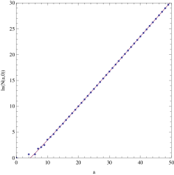
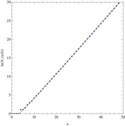
Applied to our case we find
to highest order. An almost identical calculation gives
These approximations are compared with the actual , in Figure 1.
2.2 The asymptotics of unrestricted states
Our next task is to compute the number of states without taking into account the restriction ,
The generating function for is simply ,
so that we find and hence and hence . For we find
whence and as well.
2.3 Asymptotics in both variables
Finally we take a look at the joint asymptotics for and large and comparable. This is in part motivated by the following curious observation: In [7], the asymptotics is calculated to be
where and are certain numerical constants of order one. This is reminiscent of an expansion of the Smarr formula for the area of a Kerr Black hole
if one identifies with and and with . is bounded by [6] so this identification would not lead out of the range of allowed spins for a Kerr black hole. It should also be noted that a similar suggestion has been before [13]. So, could it be that the states with describe rotating black holes?
There are a lot of reasons to doubt that, including that the meaning of really should be area, not mass squared, that states with are un-physical according to the framework of [4], and that there is a sophisticated treatment of rotating black holes in loop quantum gravity [15] that works quite differently. In fact we find that the asymptotics we calculate do not match this hypothesis at all, as follows:
Determining the asymptotics of multivariate sequences using generating functions is not a very well known subject and can become quite technical. There is however a beautifully developed general theory that one can rely on (see for example [16] for the generic case). We will use these results in the form presented in [17]. The upshot is that the asymptotics of the multivariate sequence in a certain direction is governed by one or more critical points, certain singular points of the generating function. In the case of a two variable generating function , critical points are given as solutions to
where gives the direction in which the asymptotics of the sequence is be taken. and have to satisfy several properties, for which we refer the reader to [17]. Which of the critical points actually contribute to the asymptotics can be determined by a straightforward but rather tedious analysis which we will circumvent here. If a critical point does contribute to the asymptotics of the sub-sequence of the multivariate sequence , it does so by a factor to highest order.
We are interested in the asymptotics of for constant. With the help of mathematica we compute the critical points for the problem at hand. There are eight critical points, all depending . Instead of doing a lengthy analysis as to which of these solutions contributes we simply pick the solution with the right limiting values at . It reads
where we have used the abbreviation
The asymptotic behavior is thus given by
| (9) |
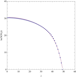
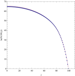
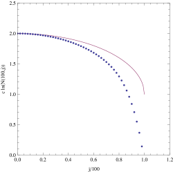
This asymptotic formula works quite well. For comparison we have plotted (9) and the actual values for two different values of .
What about the Smarr formula? We have found that, to highest order, is indeed a function of the form . However, the function is very complicated and not what one would expect if the suggested interpretation were correct. Moreover the numerical fit is quite bad, as Figure 3 demonstrates. There we have plotted the numeric result in terms of (and appropriately normalized), together with the function
| (10) |
Thus we have ample reason to throw out the hypothesis that we stated in the beginning of this subsection.
3 Conclusions
Let us summarize our results and compare them to what is known [7] about the counting for black holes using the correct area spectrum (1). To start out, all the statements made in [7] for the full spectrum are also borne out in our model on a qualitative level. In particular we see:
-
•
The number of states grows exponentially with area.
-
•
The number of (un-physical) states with arbitrary grows with same rate as that of the physical states () to highest order.
-
•
The highest order growth of and is the same.
-
•
The next to leading order term in the logarithm of the number of -states is .
This confirms the present model as a nice and simplified ‘laboratory’ for questions about the full theory. Vice versa the present note can be read as giving confirmation of the results [7]. We should however note that all the numerical factors appearing in our model are different from (although close to) the ones for the correct spectrum. To give an example, the Barbero-Immirzi-parameter obtained in [7] is whereas the one that would result if our model were correct is . This is not so surprising if one remembers a result from [6] that shows that states with higher than 1/2 certainly contribute substantially to the overall counting, however their numbers are increasingly suppressed with increasing . Thus, among all the states to be counted, the ones for which our approximation (3) is relatively bad, are most numerous.
It is curious that the coefficient of the (area)-term in the entropy seems to be very robust, as it is -1/2 in the present framework as well as in [7], [18], and elsewhere.
There is one last point worth mentioning, one that on first sight seems trivial: Since the spectrum is equidistant, the number of black hole states, and hence the entropy will grow in discrete steps. The height of the steps may vary with area, but the size of the steps is always . Surprisingly, a similar (but certainly more complex) behavior has been observed [18, 19] for the state counting in the full theory. One might at first think that this is not an accident. After all, the ‘ladder’ observed in [18, 19] may perhaps be understood as a perturbation of the half integer steps in the present model, much as the full spectrum (1) can be viewed as a perturbation (3) around the equidistant one. We will investigate this point in much more detail in a forthcoming paper [20]. The upshot is that the explanation of the ‘ladder’ is not that simple. It is related to properties of the area spectrum, in particular also to (3), but in a rather involved way.
Acknowledgements
I want to thank Willem Westra for suggesting the use of generating functions and for a lot of help in learning how to use them. I am grateful to Parthasarathi Mitra for pointing out an error in the bibliography of an earlier version of this paper.
I also gratefully acknowledge funding for this work through a Marie Curie Fellowship of the European Union.
Appendix A An alternative modified area spectrum
The form of the modified area spectrum (2) in the main text was chosen so as to approximate the actual spectrum arising in loop quantum gravity as good as possible while affording drastic simplification by being equidistant. There is another equidistantly spaced modification of the area spectrum that has been considered in the literature. It differs form (2) by removing the constant ,
| (11) |
It can be argued that this spectrum does arise in loop quantum gravity, upon quantizing the area of a non-rotating black hole following an alternative route [8].444This alternative quantization is only possible for the black hole horizon. For other surfaces, only (1) applies. In this appendix we will derive results for the asymptotic behavior of the entropy obtained with the spectrum (11). We will however be more terse than in the main text. We will get rid of all units and some constants by considering the quantity
A useful way to think about this is the following: is the number of ways to move, in an arbitrary number of steps, on the integer lattice , from the point to the point , such that the total length of the path is .
The numbers obey a recursion relation similar to the ones given in [7]. Up to simple changes of variables, they are A035002 in [21], and they are closely related to the combinatorial problems in [22].555See especially Section 7 in [22] where the object under study is essentially .
It is simple to calculate for low using a computer. Here are the first few values:
where runs horizontally and vertically.
The one step generating function for is
| (12) |
The generating function for paths with steps is just , and thus we get for the generating function for
A.1 The asymptotics of
The generating function for is (formally) the coefficient of in ,
where is a certain contour. Poles of are
with residues
Choosing the contour around and gives
The singularities suggest that to leading order. ‘Darboux’s lemma’ confirms this. We find indeed
to highest order.
A.2 The asymptotics of unrestricted states
Our next task is to compute the number of states without taking into account the restriction ,
The generating function for is simply ,
so that we find and hence .
A.3 Extremal states
Out of curiosity, let us also calculate the number of ‘extremal configurations’, . It this is easiest by going back to (12) and modifying it appropriately. In this case we only need one variable and we have
whence
(This is the well known formula for the number of ordered partitions of an integer .) Hence and .
A.4 Asymptotics in both variables
Finally we take a look at the asymptotics of for constant. With the help of Mathematica we compute the critical points for the problem at hand. There are four critical points, all depending . Instead of doing a lengthy analysis as to which of these solutions contributes we simply pick the solution with the right limiting values at . It reads
where we have used the abbreviation
The asymptotic behavior is thus given by
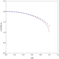
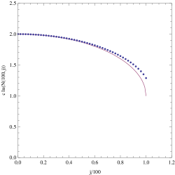
What about the Smarr formula in this case? We have found that, to highest order, is indeed a function of the form . However, the function is very complicated and not what one would expect if the suggested interpretation were correct. However, the situation is not catastrophic either: In Figure 4 we have plotted the numeric result in terms of (and appropriately normalized), together with the function
| (13) |
One sees that the numerical correspondence is not bad, but certainly not convincing.
References
- [1] T. Thiemann, “Introduction to modern canonical quantum general relativity,” arXiv:gr-qc/0110034.
- [2] A. Ashtekar and J. Lewandowski, “Background independent quantum gravity: A status report,” Class. Quant. Grav. 21 (2004) R53 [arXiv:gr-qc/0404018].
- [3] C. Rovelli, “Black hole entropy from loop quantum gravity,” Phys. Rev. Lett. 77 (1996) 3288 [arXiv:gr-qc/9603063].
- [4] A. Ashtekar, J. Baez, A. Corichi and K. Krasnov, “Quantum geometry and black hole entropy,” Phys. Rev. Lett. 80 (1998) 904 [arXiv:gr-qc/9710007].
- [5] A. Ashtekar, J. C. Baez and K. Krasnov, “Quantum geometry of isolated horizons and black hole entropy,” Adv. Theor. Math. Phys. 4 (2000) 1 [arXiv:gr-qc/0005126].
- [6] M. Domagala and J. Lewandowski, “Black hole entropy from quantum geometry,” Class. Quant. Grav. 21 (2004) 5233 [arXiv:gr-qc/0407051].
- [7] K. A. Meissner, “Black hole entropy in loop quantum gravity,” Class. Quant. Grav. 21 (2004) 5245 [arXiv:gr-qc/0407052].
- [8] J. Lewandowski, personal communication.
- [9] I. B. Khriplovich, “Holographic bound and spectrum of quantized black hole,” arXiv:gr-qc/0411109.
- [10] T. Tamaki and H. Nomura, “Ambiguity of black hole entropy in loop quantum gravity,” Phys. Rev. D 72 (2005) 107501 [arXiv:hep-th/0508142].
- [11] A. Ghosh and P. Mitra, “Counting black hole microscopic states in loop quantum gravity,” Phys. Rev. D 74 (2006) 064026 [arXiv:hep-th/0605125].
- [12] A. Ghosh and P. Mitra, “An improved lower bound on black hole entropy in the quantum geometry approach,” Phys. Lett. B 616 (2005) 114 [arXiv:gr-qc/0411035].
- [13] K. Krasnov, “Quanta of geometry and rotating black holes,” Class. Quant. Grav. 16 (1999) L15 [arXiv:gr-qc/9902015].
- [14] H.S. Wilf, Generatingfunctionology, 2nd ed., Academic Press, Boston 1994 [also available online from the homepage of its author]
- [15] A. Ashtekar, J. Engle and C. Van Den Broeck, “Quantum horizons and black hole entropy: Inclusion of distortion and rotation,” Class. Quant. Grav. 22 (2005) L27 [arXiv:gr-qc/0412003].
- [16] R. Pemantle and M. C. Wilson, “Asymptotics of multivariate sequences I: smooth points of the singular variety,” Journal of Combinatorial Theory A 97 (2002), 129.
- [17] A. Raichev and M. C. Wilson, “A new method for computing asymptotics of diagonal coefficients of multivariate generating functions,” Preprint: arXiv:math/0702595.
- [18] A. Corichi, J. Diaz-Polo and E. Fernandez-Borja, “Black hole entropy quantization,” Phys. Rev. Lett. 98 (2007) 181301 [arXiv:gr-qc/0609122].
- [19] J. Diaz-Polo and E. Fernandez-Borja, “Note on black hole radiation spectrum in Loop Quantum Gravity,” arXiv:0706.1979 [gr-qc].
- [20] H. Sahlmann, “Toward explaining black hole entropy quantization in loop quantum gravity,” arXiv:0709.2433 [gr-qc].
- [21] N. J. A. Sloane, The On-Line Encyclopedia of Integer Sequences, 2007, published electronically at www.research.att.com/njas/sequences/.
- [22] C. Coker, “Enumerating a class of lattice paths,” Discrete Mathematics 271 (2003) 13