Gravity localization on thick branes: a numerical approach
Abstract:
We introduce a numerical procedure to investigate the spectrum of massive modes and its contribution for gravity localization on thick branes. After considering a model with an analytically known Schroedinger potential, we present the method and discuss its applicability. With this procedure we can study several models even when the Schroedinger potential is not known analytically. We discuss both the occurrence of localization of gravity and the correction to the Newtonian potential given by the massive modes.
1 Introduction
In this work we deal with (4+1)-dimensional actions describing a scalar field coupled to gravity which leads to brane solutions with a single extra dimension [1, 2, 3, 4, 5, 6]. As one knows, after an Ansatz is given for the metric, minimization of the action leads to a system of second-order differential equations for the field and the metric parameter related to the warp factor. With a convenient choice of the potential one can obtain a system of first-order equations, which helps to find analytic solutions for the metric and field.
In this scenario, fluctuation around the solutions for the metric and scalar field can be decoupled in the transverse traceless gauge. After dropping the (3+1)-dimensional plane wave components, considered to satisfy a Klein-Gordon equation, the extra-dimension component of the metric fluctuations is reduced to a Schroedinger-like equation with an infinite number of solutions. Each solution is assigned to a massive mode characterized by the mass-shell condition imposed after the separation of the contribution of the four standard dimensions from the fifth or extra dimension.
In order to obtain the Schroedinger-like equation one usually goes to a conformal variable related to the extra dimension. However, it occurs that such a transformation is not always possible to be obtained analytically, and this may lead to a Schroedinger potential which is not known analytically for most of problems considered in the literature. Also, even when one knows the Schroedinger potential analytically, the whole spectrum of massive modes is hard to be obtained and normalized properly in order to study the main correction to the Newtonian potential.
In the literature, Ref. [4] has already shown that any of the following two conditions is sufficient to prove the occurrence of gravity localization, namely one has to: i) consider the zero-mode, its normalization and asymptotic behaviour or ii) analyze the asymptotic behaviour of the Schroedinger potential. For instance, both procedures were used in Ref. [7] to confirm gravity localization in a specific class of models.
However, besides confirming the occurrence of gravity localization in a model, it is of physical significance to estimate the first-order corrections to the Newtonian potential. This can be related to the limit imposed by experiments on gravity at short distances [8]. In this direction, Ref. [4] also presented an asymptotic analysis for the massive modes in a class of potentials that falls off as far from the brane; as a result, a correction of the order of is found. The issue is that corrections to the Newtonian potential for analytical Schroedinger-like potentials can in principle be found in a similar way. However, it is not rare to face problems in which the Schroedinger-like potentials are only known numerically, and in such cases the above procedure cannot be used anymore. This poses the question on how one can generate and normalize properly the massive modes in order to obtain the corrections to the Newtonian potential. The issue has motivated us to investigate the problem, and to propose the present procedure. Our numerical study shows that in order for the spectrum of massive modes to be obtained properly one must apply the normalization procedure with great care. A wrong choice of the plane wave normalization can lead to a misunderstanding of the pattern of the distribution of the massive modes and to a wrong prediction of the corrections.
In the present work, in the next Sec. 2 we deal with the equations one needs to build a Minkowski brane and to study the corresponding fluctuations in the metric and scalar fields. In Sec. 3 we review the analytic model of Ref. [5] and there we introduce the numerical method for the corrections of the Newtonian potential. A comparison of our result and the asymptotic analysis of [4] is done in order to evaluate the precision of the method. We then discuss in Sec. 4 some models with analytically known Schroedinger potential where we apply the known asymptotic analysis method, and in Sec. 5 we study models with numerically known Schroedinger potential, where we apply our numerical method. A comparison between the results coming from the numerical method and the asymptotic analysis is done. Also a comparison between the results coming from the numerical Numerov method and a simpler Euler method also available for non-analytic potentials is done. We end this work in Sec. 6, where we include some conclusions and perspectives of future investigations. A short review of the Numerov method for determining the massive modes is presented in an Appendix.
2 The brane equations and fluctuations
We start with
| (1) |
where and the metric
| (2) |
describes a background with 4-dimensional Poincare symmetry with as the extra dimension. Here and is the warp factor. We suppose that the scalar field and the warp factor only depend on the extra coordinate .
The action given by Eq.(1) leads to the following equations for the scalar field and the function from the warp factor:
| (3a) | |||||
| (3b) | |||||
| (3c) | |||||
where the prime is used to represent derivative with respect to .
The potential is supposed to have the form
| (4) |
where is in principle an arbitrary function of the field – in the supersymmetric context is named superpotential. The particular relation between and in (4) leads to a description in terms of a set of first-order differential equations, which are given by [3, 5]
| (5a) | |||||
| (5b) | |||||
We consider now the effective 4-dimensional gravitational fluctuations in the conformally flat background discussed previously, as well as the fluctuation of scalar fields around solutions of the first-order equations (5); that is, we write:
| (6) |
and we set where and represent the fluctuations and is a small parameter. On the transverse traceless gauge the metric perturbation separates from the scalars [3], leading to
| (7) |
with being the -dimensional d’Alembertian.
This equation can be decoupled by separating the 4-dimensional plane wave perturbations from the extra dimension contribution. We introduce a new variable that turns the metric into a conformal one. This changes the equation for the extra dimension contribution of the metric perturbations in a Schroedinger-like form, where no single derivative terms are present. The new conformal coordinate is defined by
| (8) |
The separation of variables is taken as
| (9) |
which turns Eq. (7) into a Klein-Gordon equation for the 4-dimensional components of the transverse-traceless , with the remaining Schroedinger-like equation
| (10) |
where we have dropped the indices from the wavefunctions, now labeled by the corresponding energy . Here the Schroedinger-like potential is given by
| (11) |
and this ends our revision of the standard braneworld scenario.
3 An analytic volcano potential
Before going into the issue concerning our numerical procedure, let us first consider the construction of a simple analytic potential characteristic of gravity localization. According to [4], for potentials constructed with the procedure of Eq. (11) that go to infinity as have this property. Also, in order to have a volcano structure we need the two components of the rhs of (11) with opposite signs. A simple choice for is
| (12) |
which is depicted in Fig. 1. In this case Eq. (11) gives the related Schroedinger-like potential
| (13) |
which is also shown in Fig. 1
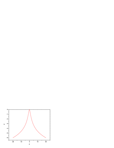
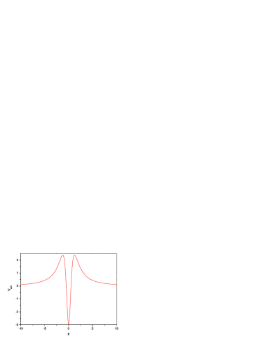
The characteristic volcano shape of the potential leads to the thick brane solution, so it contributes to smooth the potential considered in the original Randall-Sundrum [1] model which describes the thin brane solution. The analytic structure of eases the investigation of gravity localization. In particular, the zero-mode is determined analitically as
| (14) |
where is a normalization constant.
3.1 Reconstructing the model
Before turning to the gravity localization issue, let us first reverse the investigation and work on the reconstruction of the model. This means to obtain the functions , , and once is given. We hope that this reconstruction process will give us insights on the importance of in the far-reaching region for gravity localization.
We first consider Eq. (8) and write
| (15) |
Suppose we can write analytically in order to change the representation as . In this way we can invert Eq. (8) and write, in the present case
| (16) |
We invert this relation to write
| (17) |
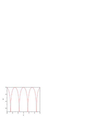
which we plot in Fig. 2. We use it in Eq. (12) to get
| (18) |
which shows – see Fig. 2 – that the variable is allowed to vary continuously only when spanning finite intervals, characterizing an effective compactification of the extra dimension in this representation.
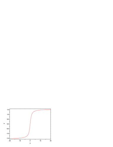
The warp factor is shown in Fig. 3. There we see that it goes to zero far from the brane, as usual, but here this happens in a finite distance from the brane, achieving the characteristic space in this region.
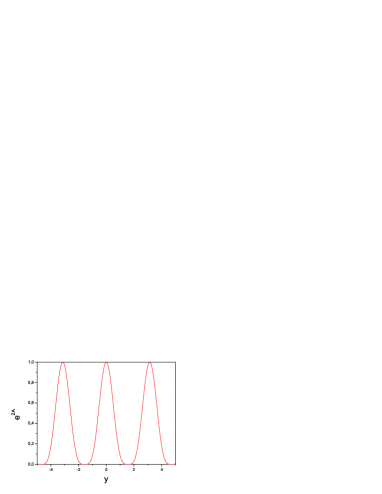
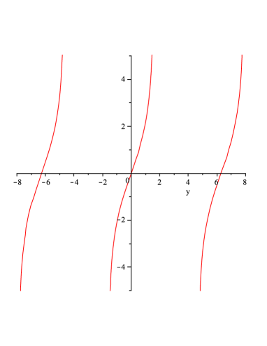
The formation of a natural barrier on the extra dimension must also be seen in the solution of the scalar field . In order to recover this, we turn attention to Eqs. (5). Differentiating Eq. (18) with respect to and substituting in Eq. (5b) gives . We can differentiate this to get . We now use Eq. (5a) to obtain
| (19) |
In Fig. 3 one sees that there are finite intervals of in which the function is not defined, and the brane has a diffuse structure. This can be better observed if we turn back to the coordinate; we write
| (20) |
which is plotted in Fig. 4, showing the kinklike profile corresponding to a difuse wall, as it appears in the vacuumless potential investigated in [9].

In this case the superpotential can also be analytically determined in the following way. An ordinary differential equation of first order for is obtained after using Eqs. (5) and derivatives of in Eq. (18) and of in Eq. (19). The procedure leads to . We solve this equation to obtain
| (21) |
with being a free parameter. The potential is then given by
| (22) |
The analytic model is very nice, and it leads us to go forward or backward very nicely.
3.2 Massive modes
Now we turn back to the Schrodinger-like equation with the aim to study the massive modes. As one knows, in the present scenario it is important to find the full spectrum of massive modes. The issue is of greater importance within the context of local localization of gravity [10]. Although it is not always possible to find analytical expressions for the massive modes [11], the analytical form of the potential helps us very much to control the numerical investigation. Indeed, a simple Runge-Kutta routine can be used with the boundary conditions and . The first condition is arbitrarily fixed, and will be adjusted with the normalization procedure. As one knows, the conformal variable leads to a probabilistic interpretation for and one must impose the condition
| (23) |
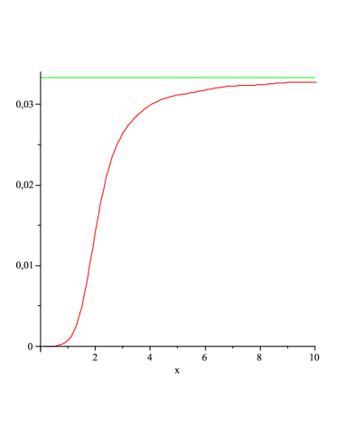
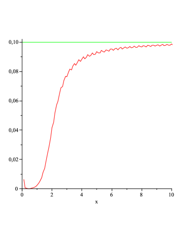
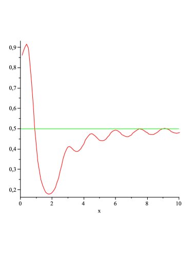
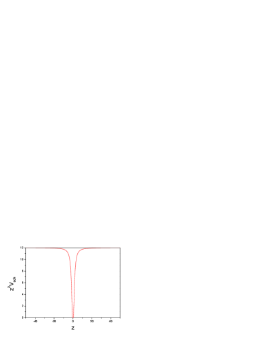
We normalize the wavefunctions in a box of size . However, an important point is to consider a box with sufficiently large size in order for the potential to achieve the regime. In fact, as already noted in [4], localization of gravity is determined by the far region of the potential. As we can see in Fig. 4, for the choice of the asymptotic regime is achieved for . In this way we must choose an at least comparable size for our box in order to correctly reproduce the gravitational features. However, to illustrate possible mistakes within the procedure, we will consider boxes of different sizes, to see spurious effects which can be observed for small boxes. We plot some results in Fig. 5, where we show the normalized as a function of for , and . Note that for we achieved the asymptotic regime for the behaviour for the potential. On the other hand, for smaller values of , say , besides a first small peak, small perturbations resembling resonances start to appear. This behaviour is greatly reinforced for . Clearly there are no resonances at all in this problem, the effect just observed being a consequence of a wrong choice of the size of the box, which could not accommodate the correct behavior of the potential
Let us now turn to asymptotic analysis in order to evaluate the degree of accuracy of our Fig. 5, for . First of all, note that in this region the factor increases monotonically with achieving a plateu for larger masses. The very existence of this plateau is confirmed after considering in the Schroedinger equation, Eq. (10). Indeed, in this case it reduces to
| (24) |
with solution . After normalization in a box one obtains for large , which for gives . See Fig. 5 for the accuracy of this limit.
Now let us consider the regime of lower modes. According to Ref. [4] – see particularly Sec. 4 –, this regime is related to the behaviour of . Indeed, in our case we have the limit . This has the particular form already proposed in Ref. [4]. There, it is shown that when this occurs one expects the lower massive modes to obey the relation . For our potential we have and this leads to . In order to look for this power law behavior in we plot in Fig. 6 the former results of Fig. 5 for in a logarithmic scale, focusing on the lower modes.
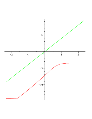
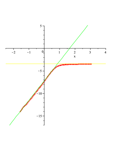
Note that the desired behaviour for small masses is obeyed in the model for almost two orders of magnitude. However, for very small masses, say for , the approximation breaks down, indicating the formation of a first small peak already noted in Fig. 5. Our simulations show that the region of validity of the approximation is enlarged toward smaller masses when the parameter is increased. Qualitatively, this can be understood very easily, since the wavefunctions have larger wavelenghts for smaller masses. As a consequence, the wavefunctions in this region do not oscillate sufficiently in the box and the procedure of normalization cannot be justified. With this reasoning, the procedure of carrying out the integration of massive modes to obtain the Newtonian potential must be done with great care, in order to eliminate the wrong contribution of modes for One possible solution, justifiable by our asymptotic analysis, is to extrapolate the observed polynomial behaviour toward the region , as shown in the right panel of Fig. 6.
3.3 Gravity localization: numerical procedure and asymptotic analysis
Let us now investigate the Newtonian potential for two masses and separated by a distance . In order to obtain the potential one sums the tower of Kaluza-Klein excitations to the usual contribution coming from the zero-mode as [4]
| (25) |
where represents the four dimensional coupling, is the fundamental five dimensional Planck scale and the integration is done considering the brane position at , as it is done in the thin brane case. Separating the contributions of the Einstein-Hilbert action due to the four dimensional part and the extra dimension, we are led to an expression relating the two scales as [4]
| (26) |
where , after the normalization procedure given by Eq. (23) is applied to the zero-mode Eq. (14). In this way, Eq. (25) can be written as
| (27) |
Note that in order to obtain the Newtonian potential for a given separation it is sufficient for practical purposes that the integration goes over the massive modes until masses of . For higher distances a considerable simplification is achieved, but for lower distances one must consider higher massive modes. In the limit, for we must integrate all possible masses until . In this way, another extrapolation of the obtained data for is necessary for higher modes. Namely, one needs to extrapolate the results displayed in Fig. 6, right panel, as .
Let us now deal with gravity localization from the asymptotic analysis of . We can separate the regime , valid for smaller masses from the regime , valid for larger masses. The constants and can be learned from Fig. 6, right panel. This figure shows that the transition region can be located at . In this way we can separate both contributions for the Newtonian potential as follows
| (28) |
For the model under investigation we have and this leads to
| (29) | |||||
and for we can write
| (30) |
which reproduces the Newtonian potential for large values of R. We then learn from this expression that the present model reproduces the known gravitational limit at large distances, localizing gravity with a correction.
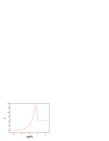
However, the full integration of Eq. (28) is still necessary in order to estimate the accuracy of our procedure. This is important in case the potential is not analytically know and also to find the value of the parameter . To implement this, we fit numerically the logarithmic plot of Fig. 6, right panel; we did that considering that it comes approximately as a superposition of two straight lines, one for each region where and . We remark that this is important in order to better achieve a control for models where the Schroedinger potential are not known analytically. First of all we get from a linear fitting of the Fig. 6, right panel, the result , leading to , giving . From the same figure we can estimate as the value of corresponding to the crossing of both straight lines for larger and smaller masses. This gives , or . Also, we find for the region the limit . After substituting these results in Eq. (28) and performing the integration, we can find the correction coefficient for , which is displayed in Fig. 7. The numerical results give a correction for large distances, which is to be compared with as the value which comes from the asymptotic analysis.
3.4 The Numerov method
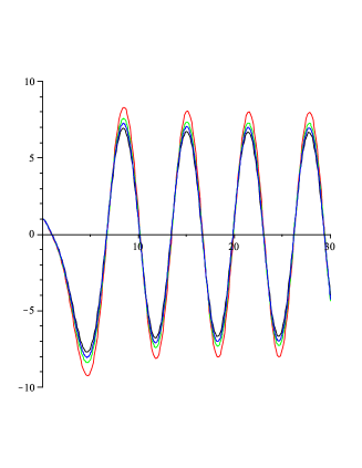
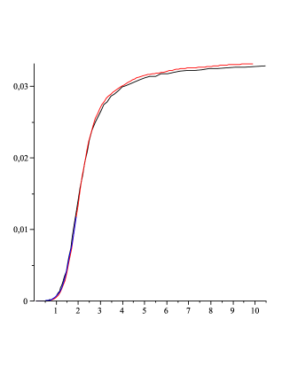
We can solve the same problem for the massive modes using the Numerov method [13] instead of the Runge-Kutta fourth-order method that we have just used. The Numerov method – see Appendix – is largely used in order to look for bound states in quantum mechanics. We can also apply it here, and some results for this model are displayed in Fig. 8. Despise the slow convergence of the Numerov method compared with Runge-Kutta methods, we can use the Numerov method when the Schroedinger potential is only known numerically.
The right panel in Fig. 8 shows a good visual concordance between both methods for as a function of m. However, in the former subsection we have emphasized the importance of the lower massive modes for gravity localization. A careful analysis in a logarithmic scale has shown that for small masses, the discrepancy between the methods grows, with Numerov method tending to present with a higher power law than the Runge-Kutta method. Naturally, this may reflect on predicting a correction to the Newtonian potential with a higher power law.
We will use this method in Sec. 5 for some other models, where the Schroedinger-like potential is only known numerically, since there the Runge-Kutta method cannot be used anymore.
4 Models with analytic : asymptotic analysis
If we compare with the presented numerical procedure, the asymptotic analysis [4] has very good precision to estimate the power of the first correction to the Newtonian potential. However, the study can only be done when one knows an analytical relation for To make this point clearer, let us illustrate this possibility with the following examples, recently considered in Ref. [12].
4.1 The case
For this model we have
| (31) |
In general this model does not give an analytic relation for However, for we get
| (32) |
with
| (33) |
This model gives an analytic expression for , depending on two parameters and :
| (34) |
In this way, we can apply the asymptotic analysis in order to study the Newtonian potential. In fact, we have the limit
| (35) |
We see from the former expression the independence of the potential of the parameters and for large values of . Following the former section we can write for Thus, and we expect that for small masses. This gives the same correction for the Newtonian potential as in the Randall-Sundrum model.
4.2 The case
For this model we have
| (36) |
For we can obtain an analytic expression for , namely
| (37) |
Inverting this expression and substituting in the expression for we get
| (38) |
For this model we have an analytic expression for the Schroedinger potential
| (39) |
with the limit
| (40) |
This limit leads to the same asymptotic result of the former section, where and , with a correction to the Newtonian potential.
5 The case of models with numerical
For a large class of models there is no analytic solution for . In this way, the analysis of and the potential must be done numerically with no a priori asymptotic analysis available to guide us. In this case the method presented in this work may be used to estimate the behavior of for small masses and to find the first correction to the Newtonian potential. We illustrate the procedure with some examples.
5.1 The case
This model gives [12]
| (41) |
We choose and write to get
| (42) |
and now we study the influence of on gravity localization. In this case, even the relation given by Eq. (15) for is not possible to be obtained analytically. Thus, we have integrated it numerically for some values of c, leading to a numerical determination of which we show in Fig. 9. Gravity localization is confirmed after demonstrating normalization of the zero-mode, as we also show in Fig. 9. We have repeated the same analysis in a logarithmic scale, and the results shown that the zero mode is nicely normalized as it goes to zero faster than , thus confirming the occurrence of gravity localization.
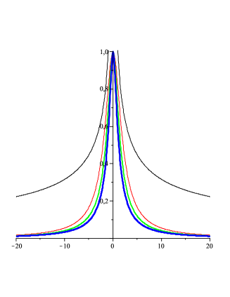
In order to study details of gravity localization one must construct the potential . We did this in Fig. 10, extending the axis in order to guarantee that the asymptotic regime is correctly achieved and that the higher massive modes can be properly normalized. Fig. 10 shows that even without an analytic expression for it indicates that asymptotically one has , and that this regime is better achieved for larger values of . In particular, for the case we have found for the limit of the value which gives .
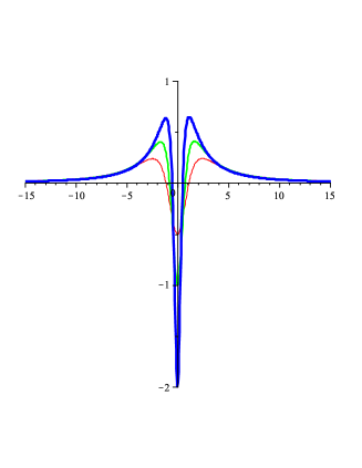
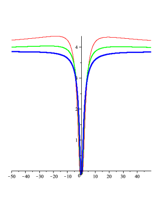
In Fig. 11, upper panel, we show the normalized probability on the brane as a function of . We see that for lower values of (red thin line) the influence of massive modes increase faster than for higher values of (blue thick line). This effect shows that gravity is easier localized for higher values of , in agreement with the results shown in Fig. 9.
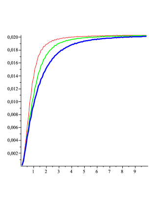
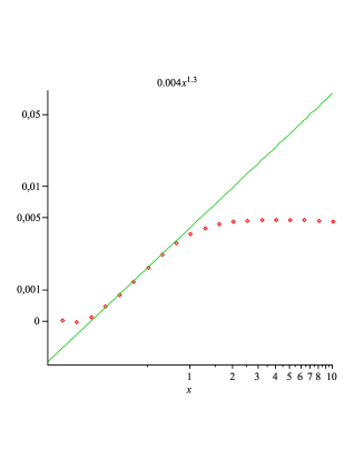
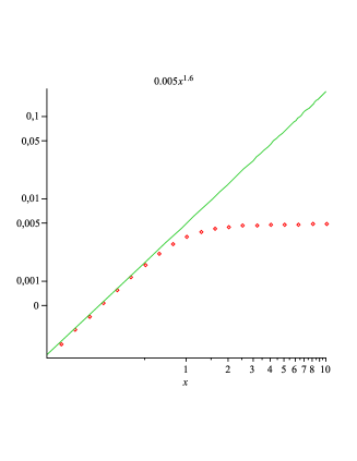
Now, the behavior of for leads to for lower masses. We compare this result with the one shown in Fig. 11, left, the green line which represents the best fit for lower masses, obtained after neglecting the very low points. In this figure, we show the logarithmic plot of as a function of , after considering with step using the Euler method for determining the massive modes. Note that, as the number of iteractions increased, it is important to find with higher precision the points corresponding to with fixed step. The plot indicates the appearance of a power law for lower masses, with , or after using , .
The very same simulation with Numerov method gives or – see Fig. 11, right panel. We notice that the Numerov method produces consistent results both for higher and lower masses, as we would expect from a higher precision method. On the contrary, the Euler method deviates from expected results in those limits due to error propagation. However, as the simpler Euler method gives fast results, it was used as a guide to search for the adequate regions to apply the Numerov method. In this way, we found two complementary numerical estimations for the correction for the Newtonian potential for large distances, , leading us to the results and . These results are to be compared to which was produced by asymptotic analysis of the Schroedinger potential.
5.2 The case
For this model we have
| (43) |
In general one cannot obtain an analytic expression for . However, for we can use the exponential integral to write
| (44) |
but we have been unable to invert this expression in order to get an analytic expression for .
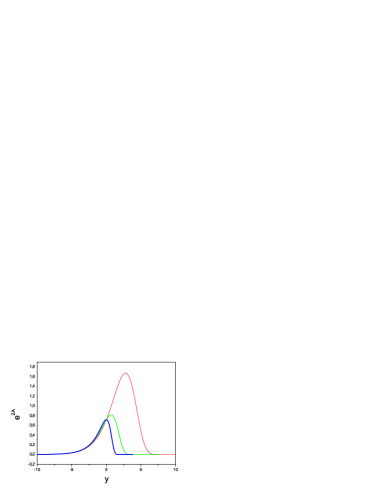
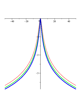
In general, this class of models leads to an asymmetric warp factor. In particular, for negative values of the warp factor goes to zero at a negative value whose module increases for smaller values of . An illustration of this is given in Fig. 12 for , in which one depicts the obtained warp factor. The figure shows the asymmetry of the constructed brane, and also the influence the factor induces on the positive region, with a maximum warp factor that increases for lower values of . The case of asymmetric brane has been studied in [14].
The asymmetry of this model poses interesting questions concerning the influence of the asymmetry on gravity localization, since it leads to an asymmetric function as well as an asymmetric . Usually, the massive modes tend to acquire the characteristics of plane waves far from the brane and the normalization for symmetric models is realized after considering a symmetric box with length . For asymmetric models, however, the normalization procedure for the massive modes must be done with care and will be postponed to a future investigation.
6 Conclusions
In this work we have investigated gravity localization in diverse braneworld models. In general, we can classify the models into two distinct classes, one which leads to analytic Schroedinger-like potential, and the other, in which the Schroedinger-like potential cannot be given analytically. The first class of models is very important, and it was nicely studied in Ref. [4], where an interesting procedure to fully investigate stability, with a very nice recipe to qualify gravity localization and Newtonian correction and to quantify the Newtonian correction.
However, there are interesting models which lead to Schroedinger-like potentials that cannot be given analytically. For such models, however, the method developed in [4] cannot be used to obtain the massive models, thus inducing a gap on the study of gravity localization in braneworld models. This problem is yet more important within the context of local localization of gravity [10], since there the knowledge of the massive modes is crucial to understand the local localization of gravity. This fact has inspired us to propose the present study, to close the aforementioned gap in the braneworld proposal.
In the course of our investigations, we had to face several interesting issues, among them we would like to pinpoint the following:
-
1.
In the Schroedinger-like equation, in order to correctly normalize the eigenfunctions we have to properly choose the size of the box, the As we have shown, we have to deal with this with care, in order to prevent the inclusion of fake resonant states.
-
2.
When the Schroedinger-like potential may be obtained analytically, a comparison between the Runge-Kutta and Numerov methods was done. In this case, the Runge-Kutta method was applyed directly as a default method for Maple, with an absolute error that can be easily fixed to a small value. As expected, the best fit between both methods is for Numerov method with smaller steps .
-
3.
When the Shroedinger-like potential is analytically known, the asymptotic analysis is the best choice in order to obtain the power law of the first correction to the Newtonian potential.
-
4.
Despide the Numerov method being the best method used to find bound states, its precision is reduced when one changes from a boundary condition problem to a initial value problem. However, its stability is best seen when compared to Euler method. Also, the Runge-Kutta method appears to be inadequate when the potential is not known analytically.
We believe that the present study contributes to enlarge the scope of stability in the braneworld scenario in the presence of large extra dimensions. The importance of the numerical procedure widens with the current interest on asymmetric branes, since there the extra dimension drives the system to behave differently, depending on the positive or negative sense one spans the fifth dimension. We hope to return to this subject in another work, investigating the presence of massive modes for asymmetric branes.
Acknowledgements: The authors would like to thank F.A. Brito and R. Menezes for discussions, and CAPES, CNPq, PADCT-MCT-CNPq, and PRONEX-CNPq-FAPESQ for financial support.
References
- [1] L. Randall and R. Sundrum, Phys. Rev. Lett. 83, 4690 (1999) [arXiv:hep-th/9906064].
- [2] W.D. Goldberger and M.B. Wise, Phys. Rev. Lett. 83, 4922 (1999) [arXiv:hep-ph/9907447]; J. Garriga and T. Tanaka, Phys. Rev. Lett. 84, 2778 (2000) [arXiv:hep-th/9911055].
- [3] O. DeWolfe, D.Z. Freedman, S.S. Gubser and A. Karch, Phys. Rev. D 62, 046008 (2000) [arXiv:hep-th/9909134].
- [4] C. Csaki, J. Erlich, T. Hollowood and Y. Shirman, Nucl. Phys. B 581, 309 (2000) [arXiv:hep-th/0001033]; C. Csaki, J. Erlich, C. Grojean, and T. Hollowood, Nucl. Phys. B 584, 359 (2000) [arXiv:hep-th/0004133].
- [5] K. Skenderis and P.K. Townsend, Phys. Lett B 468, 46 (1999) [arXiv:hep-th/9909070]; M. Gremm, Phys. Lett. B 478, 434 (2000) [arXiv:hep-th/9912060]; M. Porrati, Phys. Lett. B 498, 92 (2001) [arXiv:hep-th/0011152]; F.A. Brito, M. Cvetic, and S.-C. Yoon, Phys. Rev. D 64, 064021 (2001) [arXiv:hep-th/0105010]; M. Cvetic and N.D. Lambert, Phys. Lett. B 540, 301 (2002) [arXiv:hep-th/0205247]; S. Kobayashi, K. Koyama and J. Soda, Phys. Rev. D 65, 064014 (2002); A. Campos, Phys. Rev. Lett. 88, 141602 (2002) [arXiv:hep-th/0111207]; A. Melfo, N. Pantoja, and A. Skirzewski, Phys. Rev. D 67, 105003 (2003) [arXiv:gr-qc/0211081]; D. Bazeia, F.A. Brito, and J.R. Nascimento, Phys. Rev. D 68, 085007 (2003) [arXiv:hep-th/0306284]; D. Bazeia and A.R. Gomes, JHEP 0405, 012 (2004) [arXiv:hep-th/0403141]; K. Takahashi and T. Shiromizu, Phys. Rev. D 70, 103507 (2004) [arXiv:hep-th/0408043]; D. Bazeia, F.A. Brito, and A.R. Gomes, JHEP 0411, 070 (2004) [arXiv:hep-th/0411088].
- [6] D.Z. Freedman, C. Núñez, M. Schnabl, and K. Skenderis, Phys. Rev. D 69, 104027 (2004) [arXiv:hep-th/0312055].A. Celi et al. Phys. Rev. D 71, 045009 (2005) [arXiv:hep-th/0410126]; V.I. Afonso, D. Bazeia, and L. Losano, Phys. Lett. B 634, 526 (2006) [arXiv:hep-th/0601069]; K. Skenderis and P.K. Townsend, Phys. Rev. Lett. 96, 191301 (2006) [arXiv:hep-th/0602260]; Phys. Rev. D 74, 125008 (2006) [arXiv:hep-th/0609056]; A. Celi, JHEP 0702, 078 (2007) [arXiv:hep-th/0610300]; A. Ceresole and G. Dall’Agata, JHEP 0703, 110 (2007) [arXiv:hep-th/0702088].
- [7] D. Bazeia, C. Furtado and A.R. Gomes, JCAP 0402, 002 (2004) [arXiv:hep-th/0308034].
- [8] J.C. Long, H.W. Chan, A.B. Churnside, E.A. Gulbis, M.C.M. Varney e J.C. Price, Nature 421, 922 (2003); C.D. Hoyle, Nature 421, 899 (2003).
- [9] I. Cho and A. Vilenkin, Phys. Rev. D 59, 021701 (1999) [arXiv:hep-th/9808090] and 063510 (1999) [arXiv:hep-th/9810049]; D. Bazeia, Phys. Rev. D 60, 067705 (1999) [arXiv:hep-th/9905184].
- [10] A. Karch and L. Randall, JHEP 0105, 008 (2001) [arXiv:hep-th/0011156]; Phys. Rev. Lett. 87, 061601 (2001) [arXiv:hep-th/0105108].
- [11] N. Barbosa-Cendejas and A. Herrera-Aguilar, in Recent Developments in Gravity [arXiv:hep-th/0610052]; R. Koley and S. Kar, Phys. Lett. A 363, 369 (2007) [arXiv:quant-ph/0611068]; J. I. Diaz, J. Negro, L. M. Nieto and O. Rosas-Ortiz, J. Phys. A 32, 8447 (1999) [arXiv:quant-ph/9910017]; M. M. Nieto, Phys. Lett. B 486, 414 (2000) [arXiv:hep-th/0005281]; M. M. Nieto, Mod. Phys. Lett. A 16, 2305 (2001) [arXiv:quant-ph/0112142].
- [12] D. Bazeia, F.A. Brito, and L. Losano, JHEP 0611, 064 (2006) [arXiv:hep-th/0610233].
- [13] B. V. Numerov, Roy. Ast. Soc. Monthly Notices, 84:592, 1924. 4; J. W. Cooley, Math Comp., 15(73-76):363, 1961. 4, 8; J. M. Blatt, J. Comp. Phys., 1, 382 (1967); P. C. Show, Am. J. Phys, 40, 730 (1972); B. R. Johnson, J. Chem. Phys. 67, 4086 (1977); M. Mueller and H. Huber, Solution of the 1-D Schroedinger Equation, http://www.mapleapps.com.
- [14] O. Castillo-Felisola, A. Melfo, N. Pantoja and A. Ramirez, Phys. Rev. D 70, 104029 (2004) [arXiv:hep-th/0404083]; A. Padilla, Class. Quant. Grav. 22, 1087 (2005) [arXiv:hep-th/0406157]; K. Koyama and K. Koyama, Phys. Rev. D 72, 043511 (2005) [arXiv:hep-th/0501232]; G. Gabadadze, L. Grisa and Y. Shang, JHEP 0608, 033 (2006) [arXiv:hep-th/0604218].
Appendix: Construction of eigenfunctions of Schroedinger equation by Numerov method
Consider the Schroedinger equation
Given an energy , we look for the corresponding function , when the potential is an even function known only numerically. We follow the theoretical analysis of the renormalized Numerov method [13], where the linear character and the absence of the first derivative on the Schroedinger equation conspire to achieve a powerful sixth-order numerical method. Then, defining , we can rewrite Eq. (A.1) as . We consider the potential given as a set of points, with the variable described with fixed step This is very important and in the present case where the relation – see Eq. (8) – cannot be described analytically one needs a specific numerical procedure, where a convenient variable step on leads to a constant step on . We then expand the functions and in Taylor series in order to get
On the other hand, the second derivative of both sides of the former equation (multiplied by the convenient numerical factor ) leads to
Adding both Eqs.(A.2) and (A.3) after substituting (A.1) on the terms where the second derivative appears, we get
We now define to obtain the recurrence formula for :
We consider that the boundary condition is and that we are searching only for even modes . Then, we apply the recurrence formula for :
The condition that is even gives . In this way the former equation becomes
This result and the recurrence formula (A.5) lead us to the following strategy: we divide the interval for in slices, getting the points . Defining , we obtain . Thus, for we construct the points
in order to obtain the desired massive mode as a set of points, as we use in the text.