Efficiency of quantum Monte Carlo impurity solvers for dynamical mean-field theory

Abstract

Since the inception of the dynamical mean-field theory, numerous numerical studies have relied on the Hirsch-Fye quantum Monte Carlo (HF-QMC) method for solving the associated impurity problem. Recently developed continuous-time algorithms (CT-QMC) avoid the Trotter discretization error and allow for faster configuration updates, which makes them candidates for replacing HF-QMC. We demonstrate, however, that a state-of-the-art implementation of HF-QMC (with extrapolation of discretization $\Delta\tau\to 0$) is competitive with CT-QMC. A quantitative analysis of Trotter errors in HF-QMC estimates and of appropriate $\Delta\tau$ values is included.

I Introduction

A conventional starting point for the study of strongly correlated electron systems is the Hubbard model, which, in its single-band version, reads

$$H=-t\sum_{\langle ij\rangle,\sigma}\big{(}c_{i\sigma}^{\dagger}c_{j\sigma}^{\phantom{\dagger}}+\text{H.c.}\big{)}+U\sum_{i}n_{i\uparrow}n_{i\downarrow}\,.$$ (1)

Unfortunately, numerical methods for its direct solution are either restricted to one-dimensional cases or suffer, in general, from severe finite-size errors and/or sign problems. Insight into the physics of higher-dimensional systems, thus, requires the use of additional approximations. The dynamical mean-field theory (DMFT) neglects inter-site correlations by assuming a momentum-independent self-energy; it becomes exact in the limit of infinite coordination number. The DMFT maps the lattice problem onto a single-impurity Anderson model (SIAM), supplemented by a self-consistency condition.Georges96 Its enormous success within the last 15 years would not have been possible without the availability of controlled numerical solvers for (multi-orbital) SIAMs, in particular, of the auxiliary-field Hirsch-Fye quantum Monte Carlo (HF-QMC) algorithm.Hirsch86

The HF-QMC method discretizes the imaginary-time path integral into $\Lambda$ time slices of uniform width $\Delta\tau=\beta/\Lambda$ (at finite temperature $T=1/\beta$); a Hubbard-Stratonovich (HS) transformation replaces the electron-electron interaction at each time step by a binary auxiliary field which is sampled by standard Markov Monte Carlo (MC) techniques. The numerically costly part in each MC step is the update of the Green function ($\Lambda\times\Lambda$ matrix), which involves ${\cal O}(\Lambda^{3})$ operations. HF-QMC is numerically exact only in the limit $\Delta\tau\to 0$; raw results (for fixed $\Delta\tau$) contain the Trotter error, a statistical error (which decays as $N^{-1/2}$ for $N$ MC sweeps), and – in the DMFT context – a convergency error. Keeping $\Delta\tau$ fixed for constant accuracy, the computational cost increases as $T^{-3}$, which limits the temperature range accessible to HF-QMC. The usage of HF-QMC as a DMFT solver requires specialized techniques for Fourier transforming the time-discretized Green function; violations of causality observed in early implementationsGeorges96 may be avoided by stabilizing spline interpolations with analytic high-frequency expansions.BluemerKnecht ; Oudovenko02 ; Bluemer05ab

While fundamentally different DMFT solvers such as exact diagonalization or renormalization group methods often yield very useful information (in particular for the one-band case), they are more complementary than general alternatives to HF-QMC, e.g., for obtaining ground state or low-frequency results. Thus, much effort is being devoted to improving and extending HF-QMC, e.g., by incorporating projections to the ground stateFeldbacher04 and new HS decouplings for spin-flip terms in multi-band Hubbard models (which otherwise lead to sign problems).Sakai0406 Very recently, two novel quantum Monte Carlo approaches have been formulated for solving the impurity problem in continuous imaginary time (CT-QMC), which are based on a weak-coupling expansionRubtsov05 and an expansion in the impurity hybridization,Werner06 respectively. Each of these CT-QMC methods, which eliminate the Trotter error in HF-QMC, is a potential candidate for superseding HF-QMC as general-purpose finite-temperature DMFT solver.

The urgent need for quantitative comparisons between the CT-QMC and HF-QMC finite-temperature algorithms was soon realized. However, a first analysis of relative efficiencyGull06 suffers from using an inefficient HF-QMC-DMFT variant and neglects the essential step of extrapolating the HF-QMC results to the limit $\Delta\tau=0$. It is the purpose of this paper to show that a correction of these issues reverses the result: for the given test case of a half-filled single-band Hubbard model [Eq. (1)] with semi-elliptic density of states at low temperatures and for fixed computing resources, extrapolated HF-QMC results reach or surpass the precision of the CT-QMC methods.

II Comparisons at equal CPU time

In the following, we will extend the performance comparison initiated by Gull et al.Gull06 for the case of the interaction being chosen equal to the full bandwidth, $U=W=4$; the scale corresponds to setting $t=1/\sqrt{Z}$ in Eq. (1) on the Bethe lattice in the limit of infinite coordination number $Z$. Unless noted, all CT-QMC results shown in the following have been extracted from Ref. Gull06, . These will be compared with new HF-QMC results at equal CPU time: 140 CPU hours on common AMD Opteron compute nodes. Specifically, in the case of CT-QMC, 20 iterations of 7 hours each have been performed serially on a single AMD Opteron 244 CPU.GullPriv In the case of HF-QMC, the same fixed total CPU time has been split up among runs for 5–9 different discretizations. Keeping, for simplicity, the number of sweeps constant ($10^{6}$ per iteration), this was accomplished by adjusting the number of iterations in a range of 4–8 (which appears a bit small for reliable error analysis, but sufficient for this comparison). The advantage for the HF-QMC simulations of being run on a mix of slightly faster processorsfn:CPUs should be almost offset by their overhead of parallel execution.

Figure 1a

Figure 1: (Color online) a) Energy versus squared temperature: extrapolated HF-QMC results (circles) and estimates (Ref. Gull06, ) from CT-QMC (triangles, squares). b) Data with leading $T$ corrections subtracted, plus reference (filled circles).

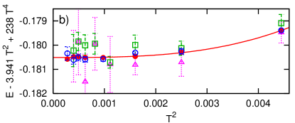
compares estimates of the energy, obtained from extrapolated HF-QMC, CT-QMC using the hybridization expansion,Werner06 and weak-coupling CT-QMC;Rubtsov05 also shown is a solid line which may be considered exact for the purpose of this comparison. Evidently, all QMC methods sustain reasonable accuracy down to fairly low temperatures $T\approx W/200$ with moderate computational cost. In order to resolve the differences, the leading temperature effects have been subtracted in Fig. 1b. At this scale, the CT-QMC results fluctuate visibly in a range consistent with their error bars, with possibly a slight positive bias for the weak-coupling variant.fn:tau In contrast, the corresponding HF-QMC results show much smaller errors and are in excellent agreement with extreme-precision HF-QMC results (filled circles).

For these reference results, 7 or 8 different discretizations using about 30–60 DMFT iterations with up to $5\cdot 10^{6}$ Monte Carlo sweeps each have been used for each temperature. All raw data points have carefully been tested for full convergence; due to the large number of iterations, autocorrelation times could be accurately determined. The HF-QMC runs for the lower temperatures have involved matrix sizes of up to $\Lambda_{\text{max}}=300$ with a computational cost of about 5000 CPU h per temperature; only for $T=1/40$ with $\Lambda_{\text{max}}=320$ the effort was higher (about 15000 CPU h). The fit curves to this data (solid lines in both panels of Fig. 1) have the form

$$E(T)=-0.18051+3.941\,T^{2}-238\,T^{4}+12746\,T^{6}.$$

Here, the leading finite-temperature correction $\tfrac{1}{2}\gamma T^{2}$ has been obtained from our estimate for the quasiparticle weight (at $T=0$, $U=4$) of $Z=0.2657\pm 0.0006$ via the relation $\gamma/2=\pi/(3Z)$; only the other 3 coefficients were free fit parameters. For this reason, our ground state estimate $E_{0}=-0.18051\pm 0.00003$ has about the same (small) error bar as the best finite–temperature data.

A direct comparison of the accuracies of the different methods is shown in Fig. 2.

Figure 2: (Color online) Comparisons of errors in QMC energy estimates: absolute deviations of the data shown in Fig. 1 from the reference curve on a logarithmic scale.

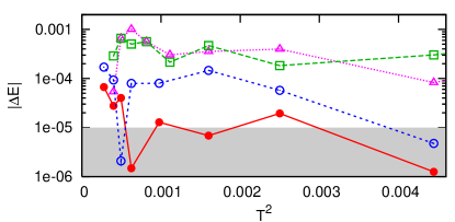
The absolute errors (determined as deviation from the reference curve) of the hybridization CT-QMC results (triangles) generally increase from $10^{-4}$ at the highest temperatures to $10^{-3}$ at lower $T$; similar behavior (with stronger fluctuations) is observed for the weak-coupling CT-QMC data (squares). Already the “regular” HF-QMC results (using 140 CPU h, open circles) are more accurate by nearly an order of magnitude, only to be surpassed by the more costly HF-QMC points (solid circles); note that all error estimates are reliable only down to the precision of the reference of about $10^{-5}$. In the following, we will highlight the methodological ingredients that allow for the high demonstrated efficiency of our HF-QMC procedure.

An essential feature of reliable HF-QMC studies is the inclusion of runs with different discretizations $\Delta\tau$ for estimating the impact of the associated systematic error; high-precision HF-QMC results can only be obtained by extrapolations $\Delta\tau\to 0$ as illustrated in Fig. 3a:

Figure 3: (Color online) a) HF-QMC estimate of energy at $T=1/45$ (circles) versus discretization $\Delta\tau$ with extrapolation $\Delta\tau\to 0$ (dashed line). b) Same data after subtraction of approximate leading $\Delta\tau$ error versus $\Delta\tau^{2}$ in comparison with reference HF-QMC data (filled circles and solid line).

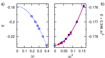
The raw HF-QMC results for the energy (circles) vary by about $0.04$ when the discretization is reduced from $\Delta\tau=0.4$ to $\Delta\tau=0.2$. As revealed by the extrapolation (dashed line), even the best raw results still contain systematic errors of order $10^{-2}$; however, the $\Delta\tau$ error is very regular and can essentially be eliminated in a quadratic least-squares fit in $\Delta\tau^{2}$ (cf. Sec. III). Already the subtraction of the (easily estimated) leading correction (which is linear in $\Delta\tau^{2}$) reduces the errors by one order of magnitude as shown in Fig. 3b; only at this scale, the statistical error bars (of about $5\cdot 10^{-5}$) become visible. Full quadratic extrapolation (in $\Delta\tau^{2}$; dashed line) of the regular HF-QMC data results in a total error of $1.5\cdot 10^{-4}$ (empty circle at $\Delta\tau^{2}=0$), i.e., in a reduction of the initial error by two full orders of magnitude. The excellent agreement with high-precision HF-QMC data (filled circles and solid line) confirms the validity of this procedure. Note that already the standard range of discretizations $\tau\in[0.2,0.4]$ in our HF-QMC data implies matrix sizes of up to 226 (at $T=1/45$), vastly greater than typical matrix sizes of about 80 for weak-coupling and about 12 for hybridization expansion CT-QMC.Gull06

An important prerequisite for extrapolation schemes such as described above is that all errors in the raw data (for fixed $\Delta\tau$) are well under control. By Fourier transforming only the difference between the QMC estimated Green function and a reference Green function (which is exact to order $U^{2}$), our HF-QMC implementationBluemerKnecht eliminates $\Delta\tau$ errors beyond the inevitable Trotter contribution; at the same time, high-frequency fluctuations are reduced. This is illustrated in the comparison of QMC self-energy estimates in Fig. 4.

Figure 4: (Color online) Imaginary part of self-energy on the imaginary axis for $T=1/45$ as estimated by CT-QMC (Ref. Gull06, ) using the hybridization expansion (triangles) or the weak-coupling expansion (circles) and by Hirsch-Fye QMC (dashed lines for $\Delta\tau=0.4,\Delta\tau=0.2$, solid line for $\Delta\tau\to 0$).

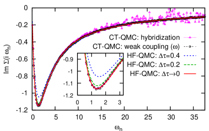
Even the HF-QMC result for the coarsest discretization $\Delta\tau=0.4$ (short-dashed line) deviates from the results for $\Delta\tau=0.2$ and $\Delta\tau\to 0$ (long-dashed and solid lines, respectively) visibly only for $\omega_{n}\lesssim 3$ (magnified in the inset). The extrapolated HF-QMC curve, in turn, agrees with the CT-QMC data at all frequencies, except for high-frequency fluctuations in the hybridization CT-QMC results.

As a consequence of the minimization of discretization errors in our HF-QMC implementation, also fluctuations in static quantities such as estimates of the kinetic energy are suppressed, as seen in Fig. 5:

Figure 5: (Color online) Kinetic energy versus squared temperature (minus leading $T$ corrections): estimates from HF-QMC at finite discretization (squares for $\Delta\tau=0.15$, diamonds for $\Delta\tau=0.2$) and after extrapolation $\Delta\tau\to 0$ (circles); dashed and solid lines denote corresponding reference results. Also shown: HF-QMC results extracted from Fig. 3 in Ref. Gull06, (crosses); thin lines are guides to the eye only.

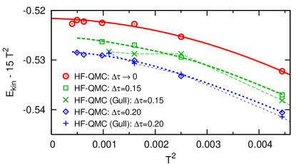
our HF-QMC results at finite discretization (squares/diamonds) follow the reference results (dashed lines) with only small scatter; thus, a reliable extrapolation $\Delta\tau\to 0$ is possible (circles and solid line). In contrast, the HF-QMC results from Ref. Gull06, (crosses) show an order of magnitude larger fluctuations and do not allow for a precise extrapolation, although they have been obtained at higher cost (140 CPU h per data point) than each of our finite–$\Delta\tau$ results (for which between 5 and 70 CPU h were used, depending on temperature). Evidently, the HF-QMC implementation used in Ref. Gull06, is much less efficient.

As seen in Fig. 6,

Figure 6: (Color online) Kinetic energy versus squared temperature: estimates at fixed CPU time from CT-QMC (Ref. Gull06, ) (triangles, squares) and HF-QMC (empty circles) after subtracting leading $T$ corrections. Also shown are higher-precision results from HF-QMC (filled circles and solid line) and hybridization CT-QMC (double-dashed line).

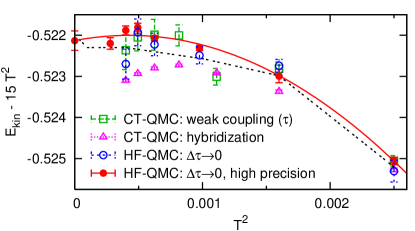
the estimates of the kinetic energy obtained from weak-coupling CT-QMC and $\Delta\tau$-extrapolated regular HF-QMC agree within their (similar) error bars with the reference HF-QMC results; the extrapolation of the latter for $T\to 0$ (solid line) is also in excellent agreement with low-$T$ hybridization CT-QMC data of Ref. Werner06, (double-dashed line). The regular hybridization CT-QMC data (triangles) shows by a factor of about 2 larger deviations from the reference (this deviation is systematic and far beyond the stated error bars). So, all 3 QMC methods show roughly the same efficiency in estimating this observable.

III Quantitative study of HF-QMC Trotter errors

As we have established above for the specific test case defined in Ref. Gull06, , HF-QMC results should be extrapolated to $\Delta\tau=0$, if possible. Many HF-QMC studies, however, include simulations only for a single value of $\Delta\tau$. The reliability of such studies depends on whether the chosen values of $\Delta\tau$ can be regarded as “small”. Up to now, many different criteria have been used in the literature, such as (for $t^{*}=1$) $\Delta\tau\lesssim 0.25$ or $\Delta\tau\lesssim 1/(5U)$ etc.Werner06 We have invested significant computing resources for determining the leading and subleading Trotter errors in HF-QMC estimates of selected observables throughout the (paramagnetic) phase space of model (1). Figure 7

Figure 7: (Color online) Coefficients of Trotter errors in HF-QMC estimates of the energy (see text).

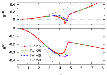
shows the coefficients in an expansion of the form

$$E(U,\!T;\Delta\tau)\approx E^{(0)}(U,\!T)+E^{(2)}(U,\!T)\Delta\tau^{2}+E^{(4)}(U,\!T)\Delta\tau^{4}$$

versus interaction $U$ for a range of temperatures extending from a value slightly above the critical Mott end point ($U\approx 4.67$, $T\approx 0.055$) to much smaller values. For weak interaction $U\lesssim 2$, both the leading correction $E^{(2)}$ (lower panel) and the subleading term $E^{(4)}$ (upper panel) scale asymptotically as $U^{2}$ (double-dashed lines); thus, in this regime the Trotter error is indeed proportional to $(U\Delta\tau)^{2}$. For larger interactions, however, the error grows much slower; it even decreases as a function of $U$ in the strongly correlated metallic phase ($4\lesssim U\lesssim 5$). Only in this range, a temperature dependence of the coefficients becomes clearly visible. Finally, in the insulating phase ($U\gtrsim 5$), the leading coefficient $E^{(2)}$ grows essentially linearly with $U$, so that $\Delta\tau\sqrt{U}$ would have to be kept constant for constant Trotter error.

The corresponding coefficients in the HF-QMC Trotter error expansion for the kinetic energy show markedly different behaviors in Fig. 8.

Figure 8: (Color online) Coefficients of Trotter errors in HF-QMC estimates of kinetic energy. Inset: relative coefficients.

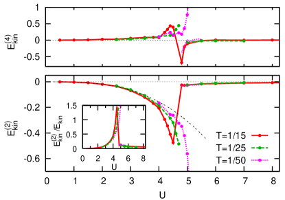
Here, the leading coefficient $E_{\text{kin}}^{(2)}$ scales as $U^{3}$ for $U\lesssim 3$; $E_{\text{kin}}^{(4)}$ is too noisy for this kind of analysis. Both coefficients are strongly enhanced near the Mott transitions, with a pole-like structure in $E_{\text{kin}}^{(4)}$. Again, the temperature dependences are appreciable only in this range. Somewhat surprisingly, the Trotter errors decay quickly in the insulating phase, even the relative errors (see inset of Fig. 8); this observation may be specific to our implementation.

In the case of the double occupancy $D=\langle n_{i\uparrow}n_{i\downarrow}\rangle$ (see Fig. 9),

Figure 9: (Color online) Coefficients of Trotter errors in HF-QMC estimates of double occupancy.

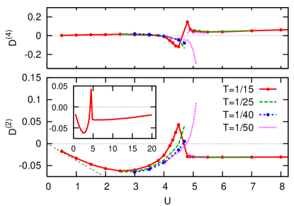
the Trotter error starts off as $\Delta\tau^{2}U$ for very small interactions $U\lesssim 1$. It then decays with a sign change just below the Mott transition. In the insulating phase, both coefficients are nearly constant; a decay of $D^{(2)}$ for extremely large $U$ is visible in the inset.

IV Conclusion

We have compared published resultsGull06 of two different continuous-time QMC methods with data obtained from a Hirsch-Fye QMC implementation by extrapolating the discretization $\Delta\tau\to 0$. HF-QMC involved typical matrix sizes more than twice as large as weak-coupling CT-QMC and nearly 20 times larger than hybridization CT-QMC (cf. Fig. 2 in Ref. Gull06, ). If this was the only relevant factor, HF-QMC should (due to the cubic scaling of the runtime of each method with the matrix size) be less efficient by one order of magnitude than the weak-coupling and by four orders of magnitude than the hybridization expansion variant. However, at (roughly) equal numerical effort, the HF-QMC results are about equally accurate for the kinetic energy and an order of magnitude more accurate for the energy; the latter translatesfn:CLT into two orders of magnitude higher efficiency of HF-QMC. Apparently, much larger fluctuations in the CT-QMC methods outweigh the advantage of using smaller matrices (in the temperature range included in this comparison). An important factor is certainly the computation of Green functions which is (on the discretization grid) trivial for HF-QMC (with $\Lambda$ measurements for each time difference $\tau_{i}-\tau_{j}$ resulting from each sweep) while it requires significant additional efforts in both CT-QMC methods.Gull06

We have also quantified contributions to the Trotter error in HF-QMC estimates of energetics which show quite complex behavior. A rule for “small enough” values of $\Delta\tau$ which holds approximately for large $U$ can be obtained by requiring the quartic corrections (for $E$ or $D$) to be smaller than the quadratic ones: $\Delta\tau\ll 1/\sqrt{0.28Ut^{*}}$. The observed small temperature dependence of the coefficients could be used for cheap high-precision studies at low $T$ (by extrapolating the coefficients and performing low-$T$ simulations only for large $\Delta\tau$). A more surprising insight is that the Trotter errors in $D$ are unusually small for $U\approx 4.8$ and $T\lesssim 40$; the same holds true for $E^{(4)}$ so that HF-QMC is particularly precise in this range. More generally, HF-QMC remains the method of choice for obtaining precise energetics, even extrapolated to the ground state.Bluemer05ab

The CT-QMC methods are certainly important and promising additions to the portfolio of DMFT impurity solvers. They allow for direct simulations at extremely low temperatures without requiring extrapolations in $\Delta\tau$ and/or $T$ and appear to offer greater flexibility in the choice of the Hamiltonian without incurring significant sign problems. However, as shown in this study, HF-QMC (with extrapolation $\Delta\tau\to 0$) can be equally or even more efficient and should not be discarded (yet).

References

- (1) A. Georges, G. Kotliar, W. Krauth, and M. Rozenberg, Rev. Mod. Phys. 68, 13 (1996).
- (2) J. E. Hirsch and R. M. Fye, Phys. Rev. Lett. 56, 2521 (1986).
- (3) C. Knecht, diploma thesis, Universität Mainz (2002); N. Blümer, Ph. D. thesis, Universität Augsburg (2002); Shaker, Aachen, 2003; C. Knecht, N. Blümer, and P.G.J. van Dongen, Phys. Rev. B 72, 081103(R) (2005).
- (4) V. S. Oudovenko and G. Kotliar, Phys. Rev. B 65, 75102 (2002).
- (5) N. Blümer and E. Kalinowski, Phys. Rev. B 71, 195102 (2005); Physica B 359, 648 (2005).
- (6) M. Feldbacher, K. Held, and F. F. Assaad, Phys. Rev. Lett. 93, 136405 (2004).
- (7) S. Sakai, R. Arita, and H. Aoki, Phys. Rev. B 70, 172504 (2004); S. Sakai, R. Arita, K. Held, and H. Aoki, Phys. Rev. B 74, 155102 (2006).
- (8) A. N. Rubtsov, V. V. Savkin, and A. I. Lichtenstein, Phys. Rev. B 72, 035122 (2005).
- (9) P. Werner, A. Comanac, L. de Medici, M. Troyer, and A. J. Millis, Phys. Rev. Lett. 97, 076405 (2006).
- (10) E. Gull, P. Werner, A. J. Millis, and M. Troyer, arXiv:cond-mat/0609438v1.
- (11) E. Gull, private communication (2006).
- (12) The HF-QMC results have been obtained by parallel executions on 8 (sometimes 16) processor cores on a mix on AMD processors (Opteron 244, 246, 270, and 2216).
- (13) Here and in the following, we show the more favorable set of weak-coupling CT-QMC results: measurement in for , measurement in for ; cf. Ref. Gull06, .
- (14) According to the Central Limit Theorem, increasing the runtime in Monte Carlo methods by orders of magnitude reduces (statistical) errors by orders of magnitude.