DESY 07-117


Next-to-leading order corrections in
exclusive meson production

M. Diehl and W. Kugler

Deutsches Elektronen-Synchroton DESY, 22603 Hamburg, Germany
Abstract
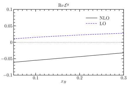
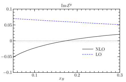
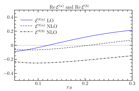
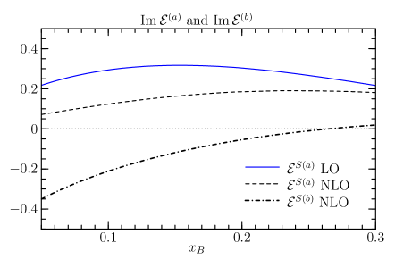
We analyze in detail the size of next-to-leading order corrections to hard exclusive meson production within the collinear factorization approach. Corrections to the cross section are found to be huge at small xBsubscript𝑥𝐵x_{B} and substantial in typical fixed-target kinematics. With the models we take for nucleon helicity-flip distributions, the transverse target polarization asymmetry in vector meson production is strongly affected by radiative corrections, except at large xBsubscript𝑥𝐵x_{B}. Its overall size is very small for ρ𝜌\rho production but can be large in the ω𝜔\omega channel.


1 Introduction

Generalized parton distributions (GPDs) have developed into a versatile tool to quantify important aspects of hadron structure in QCD. In particular they contain unique information on the transverse spatial distribution of partons [1] and on spin-orbit effects and orbital angular momentum inside the nucleon [2, 3]. Deeply virtual Compton scattering is widely recognized as the process providing the theoretically cleanest access to GPDs, with a wealth of observables calculable in the large Q2superscript𝑄2Q^{2} limit [4] and with the calculation of the hard-scattering subprocess now pushed to next-to-next-to-leading order (NNLO) accuracy in αssubscript𝛼𝑠\alpha_{s} [5]. A quantitative theoretical description of exclusive meson production remains a challenge. It would offer the possibility to obtain important complementary information, difficult to obtain from Compton scattering alone. Perhaps most importantly, vector meson production is directly sensitive to gluon distributions, which in the Compton process are αssubscript𝛼𝑠\alpha_{s} suppressed relative to quark distributions and only accessible through scaling violation (just as in the well-known case of inclusive deep inelastic scattering). Given in addition the large number of channels that can be studied and the wealth of high-quality data in a wide range of kinematics from collider to fixed-target energies [6, 7], it should be worthwhile to try and push the theory description of exclusive meson production as far as possible.

In this work we study the exclusive production of light mesons at large photon virtuality Q2superscript𝑄2Q^{2} within the framework of collinear factorization [8]. In Bjorken kinematics, the process amplitude can be approximated by the convolution of hard-scattering kernels with generalized parton distributions and the quark-antiquark distribution amplitude of the produced meson. The hard-scattering kernels have been calculated to O(αs2)𝑂superscriptsubscript𝛼𝑠2O(\alpha_{s}^{2}), i.e. to next-to-leading order (NLO) accuracy [9, 10, 11]. The aim of the present paper is to investigate in some detail the size of the NLO corrections compared with the leading-order (LO) results, on which phenomenological studies have so far relied.

The collinear factorization approach provides an approximation of the leading helicity amplitudes for meson production in the Bjorken limit, up to relative corrections of order 1/Q21superscript𝑄21/Q^{2}. These power corrections cannot be calculated systematically (and in fact the derivation [8] of the factorization theorem suggests that these corrections do not all factorize into hard-scattering kernels and nonperturbative quantities pertaining to either the nucleon or the produced meson). One particular source of power corrections can however readily be identified, namely the effect of the transverse momentum of partons entering the hard-scattering subprocess, which in the collinear approximation is neglected in the calculation of the hard-scattering kernel. A number of approaches include these kTsubscript𝑘𝑇k_{T} effects, in particular the studies in [12, 13] based on the modified hard-scattering formalism of Sterman et al. [14], and calculations like [15] which are based on the color dipole formulation. In the work by Martin, Ryskin and Teubner [16], parton-hadron duality is used to model the meson formation and thus the transverse momentum of the hadronizing quarks is included in the calculation, whereas the transverse momentum of gluons in the proton is treated within high-energy kTsubscript𝑘𝑇k_{T} factorization. The studies just quoted agree in that transverse momentum effects result in substantial power corrections to the collinear approximation for Q2superscript𝑄2Q^{2} up to several GeV2superscriptGeV2\operatorname{GeV}^{2}. Unfortunately, the calculation of full NLO corrections in αssubscript𝛼𝑠\alpha_{s} remains not only a practical but also a conceptual challenge in all of these approaches, so that the perturbative stability of their results cannot be investigated at present. (The approach of Sterman et al. takes partial account of radiative corrections, resumming a certain class of them into Sudakov form factors.)

A consistent simultaneous treatment of radiative and power corrections being out of reach at this time, a possible strategy is to study the NLO corrections in the collinear approximation and in particular to identify kinematical regions where these corrections are moderate or small. There one can then use with greater confidence formulations incorporating power corrections. In this spirit the present investigation should be understood. We will study both the cross section for meson production from an unpolarized target and the transverse target polarization asymmetry. This asymmetry is one of the few observables sensitive to the nucleon helicity-flip distributions (in particular for gluons) and hence to the spin-orbit and orbital angular momentum effects mentioned above. We will in particular see whether corrections tend to cancel in this polarization asymmetry, as is often assumed.

In the bulk of this paper we concentrate on the production of vector mesons. In Sect. 2 we set up our notation and recall important properties of the hard-scattering kernels at NLO, as well as giving a one-variable representation of these kernels after Gegenbauer expansion of the meson distribution amplitude. In Sect. 3 we specify the model of the generalized parton distributions H𝐻H and E𝐸E we use for our numerical studies. The size of radiative corrections involving convolutions with distributions H𝐻H is then studied in Sects. 4 and 5 for small and large xBsubscript𝑥𝐵x_{B}, respectively, and the convolutions involving distributions E𝐸E are quantified in Sect. 6. In Sect. 7 we then look at the NLO corrections at the level of the observable cross section and polarization asymmetry. A brief study of exclusive pion production in Sect. 8 complements our work, and in Sect. 9 we summarize our main findings. A number of more lengthy formulae is collected in appendices.

2 Hard-scattering kernels

In the main part of this paper we are concerned with exclusive production of a vector meson

γ(q)+p(p)V(q)+p(p)superscript𝛾𝑞𝑝𝑝𝑉superscript𝑞𝑝superscript𝑝\gamma^{*}(q)+p(p)\to V(q^{\prime})+p(p^{\prime}) (1)

in the limit of large Q2=q2superscript𝑄2superscript𝑞2Q^{2}=-q^{2} at fixed Bjorken variable xB=Q2/(2pq)subscript𝑥𝐵superscript𝑄22𝑝𝑞x_{B}=Q^{2}/(2p\cdot q) and fixed t=(pp)2𝑡superscript𝑝superscript𝑝2t=(p-p^{\prime})^{2}. To leading order in 1/Q1𝑄1/Q, the amplitude for longitudinal polarization of photon and meson can be written as

\displaystyle\mathcal{M} =2π4παξQNcQVfV01dzϕV(z)11dx{Tg(z,x,ξ)Fg(x,ξ,t)\displaystyle=\frac{2\pi\sqrt{4\pi\alpha}}{\xi\mskip 1.5muQN_{c}}\,Q_{V}f_{V}\int_{0}^{1}dz\,\phi_{V}(z)\int_{-1}^{1}dx\,\biggl{\{}T_{g}(z,x,\xi)\mskip 1.5muF^{g}(x,\xi,t)
+1nf[Ta(z¯,x,ξ)Ta(z,x,ξ)]FS(x,ξ,t)+Tb(z,x,ξ)FS(x,ξ,t)1subscript𝑛𝑓delimited-[]subscript𝑇𝑎¯𝑧𝑥𝜉subscript𝑇𝑎𝑧𝑥𝜉superscript𝐹𝑆𝑥𝜉𝑡subscript𝑇𝑏𝑧𝑥𝜉superscript𝐹𝑆𝑥𝜉𝑡\displaystyle\qquad+\frac{1}{n_{f}}\Bigl{[}T_{a}(\bar{z},x,\xi)-T_{a}(z,-x,\xi)\Bigr{]}\mskip 1.5muF^{S}(x,\xi,t)+T_{b}(z,x,\xi)\mskip 1.5muF^{S}(x,\xi,t)\phantom{\biggl{[}\biggr{]}}
+eV(3)[Ta(z¯,x,ξ)Ta(z,x,ξ)][Fu(+)(x,ξ,t)Fd(+)(x,ξ,t)]superscriptsubscript𝑒𝑉3delimited-[]subscript𝑇𝑎¯𝑧𝑥𝜉subscript𝑇𝑎𝑧𝑥𝜉delimited-[]superscript𝐹𝑢𝑥𝜉𝑡superscript𝐹𝑑𝑥𝜉𝑡\displaystyle\qquad+e_{V}^{(3)}\,\Bigl{[}T_{a}(\bar{z},x,\xi)-T_{a}(z,-x,\xi)\Bigr{]}\,\Bigl{[}F^{u(+)}(x,\xi,t)-F^{d(+)}(x,\xi,t)\Bigr{]}\phantom{\biggl{[}\biggr{]}}
+eV(8)[Ta(z¯,x,ξ)Ta(z,x,ξ)][Fu(+)(x,ξ,t)+Fd(+)(x,ξ,t)2Fs(+)(x,ξ,t)]}\displaystyle\qquad+e_{V}^{(8)}\,\Bigl{[}T_{a}(\bar{z},x,\xi)-T_{a}(z,-x,\xi)\Bigr{]}\,\Bigl{[}F^{u(+)}(x,\xi,t)+F^{d(+)}(x,\xi,t)-2F^{s(+)}(x,\xi,t)\Bigr{]}\biggr{\}} (2)

with z¯=1z¯𝑧1𝑧\bar{z}=1-z, Nc=3subscript𝑁𝑐3N_{c}=3, and the electromagnetic fine structure constant α𝛼\alpha. Throughout this paper we work with nf=3subscript𝑛𝑓3n_{f}=3 active quark flavors. The proton matrix elements F𝐹F are parameterized by generalized parton distributions,

Fq,g(x,ξ,t)=1(p+p)n[Hq,g(x,ξ,t)u¯(p)u(p)+Eq,g(x,ξ,t)u¯(p)iσαβnα(pp)β2mpu(p)]superscript𝐹𝑞𝑔𝑥𝜉𝑡1𝑝superscript𝑝𝑛delimited-[]superscript𝐻𝑞𝑔𝑥𝜉𝑡¯𝑢superscript𝑝italic-n̸𝑢𝑝superscript𝐸𝑞𝑔𝑥𝜉𝑡¯𝑢superscript𝑝𝑖superscript𝜎𝛼𝛽subscript𝑛𝛼subscriptsuperscript𝑝𝑝𝛽2subscript𝑚𝑝𝑢𝑝F^{q,g}(x,\xi,t)=\frac{1}{(p+p^{\prime})\cdot n}\left[H^{q,g}(x,\xi,t)\,\bar{u}(p^{\prime})\mskip 1.5mu\not{n}\mskip 1.5muu(p)+E^{q,g}(x,\xi,t)\,\bar{u}(p^{\prime})\,\frac{i\sigma^{\alpha\beta}n_{\alpha}(p^{\prime}-p)_{\beta}}{2m_{p}}\,u(p)\right] (3)

for quarks and gluons, where we use the conventions of [17]. Here n𝑛n is a light-like auxiliary vector, ξ=xB/(2xB)𝜉subscript𝑥𝐵2subscript𝑥𝐵\xi=x_{B}/(2-x_{B}) is the skewness variable, and mpsubscript𝑚𝑝m_{p} denotes the nucleon mass. We have further introduced the combination

Fq(+)(x,ξ,t)=Fq(x,ξ,t)Fq(x,ξ,t)superscript𝐹𝑞𝑥𝜉𝑡superscript𝐹𝑞𝑥𝜉𝑡superscript𝐹𝑞𝑥𝜉𝑡F^{q(+)}(x,\xi,t)=F^{q}(x,\xi,t)-F^{q}(-x,\xi,t) (4)

with positive charge conjugation parity. In (2) we have arranged the terms containing quark distributions into the flavor singlet

FSsuperscript𝐹𝑆\displaystyle F^{S} =Fu(+)+Fd(+)+Fs(+)absentsuperscript𝐹𝑢superscript𝐹𝑑superscript𝐹𝑠\displaystyle=F^{u(+)}+F^{d(+)}+F^{s(+)} (5)

and the flavor triplet and octet combinations, Fu(+)Fd(+)superscript𝐹𝑢superscript𝐹𝑑F^{u(+)}-F^{d(+)} and Fu(+)+Fd(+)2Fs(+)superscript𝐹𝑢superscript𝐹𝑑2superscript𝐹𝑠F^{u(+)}+F^{d(+)}-2F^{s(+)}. The factors

Qρsubscript𝑄𝜌\displaystyle Q_{\rho} =12,absent12\displaystyle=\tfrac{1}{\sqrt{2}}\,, Qωsubscript𝑄𝜔\displaystyle Q_{\omega} =132,absent132\displaystyle=\tfrac{1}{3\sqrt{2}}\,, Qϕsubscript𝑄italic-ϕ\displaystyle Q_{\phi} =13absent13\displaystyle=-\tfrac{1}{3} (6)

and

eρ(3)superscriptsubscript𝑒𝜌3\displaystyle e_{\rho}^{(3)} =eρ(8)=eω(8)=16,absentsuperscriptsubscript𝑒𝜌8superscriptsubscript𝑒𝜔816\displaystyle=e_{\rho}^{(8)}=e_{\omega}^{(8)}=\tfrac{1}{6}\,, eω(3)superscriptsubscript𝑒𝜔3\displaystyle e_{\omega}^{(3)} =32,absent32\displaystyle=\tfrac{3}{2}\,, eϕ(3)superscriptsubscript𝑒italic-ϕ3\displaystyle e_{\phi}^{(3)} =0,absent0\displaystyle=0\,, eϕ(8)superscriptsubscript𝑒italic-ϕ8\displaystyle e_{\phi}^{(8)} =13absent13\displaystyle=-\tfrac{1}{3} (7)

correspond to a respective flavor content

12(|uu¯|dd¯),12(|uu¯+|dd¯),|ss¯12ket𝑢¯𝑢ket𝑑¯𝑑12ket𝑢¯𝑢ket𝑑¯𝑑ket𝑠¯𝑠\tfrac{1}{\sqrt{2}}\bigl{(}|u\bar{u}\rangle-|d\bar{d}\rangle\bigr{)}\,,\qquad\tfrac{1}{\sqrt{2}}\bigl{(}|u\bar{u}\rangle+|d\bar{d}\rangle\bigr{)}\,,\qquad|s\bar{s}\rangle (8)

of the ρ𝜌\rho, ω𝜔\omega and ϕitalic-ϕ\phi. The meson distribution amplitudes ϕV(z)subscriptitalic-ϕ𝑉𝑧\phi_{V}(z) are normalized as 01𝑑zϕV(z)=1superscriptsubscript01differential-d𝑧subscriptitalic-ϕ𝑉𝑧1\int_{0}^{1}dz\,\phi_{V}(z)=1, and the decay constants have the values fρ=209MeVsubscript𝑓𝜌209MeVf_{\rho}=209\operatorname{MeV}, fω=187MeVsubscript𝑓𝜔187MeVf_{\omega}=187\operatorname{MeV}, fϕ=221MeVsubscript𝑓italic-ϕ221MeVf_{\phi}=221\operatorname{MeV} [18]. We finally have hard-scattering kernels in (2), where Tgsubscript𝑇𝑔T_{g} goes with gluon and Tasubscript𝑇𝑎T_{a}, Tbsubscript𝑇𝑏T_{b} go with quark distributions in the proton. In the graphs for Tasubscript𝑇𝑎T_{a} quark lines connect the proton and meson side, whereas in the graphs for Tbsubscript𝑇𝑏T_{b} the proton and meson side are only connected by gluon lines. Tbsubscript𝑇𝑏T_{b} thus starts at order αs2superscriptsubscript𝛼𝑠2\alpha_{s}^{2} and only goes with the quark singlet distribution FSsuperscript𝐹𝑆F^{S}. Example graphs for the three kernels at NLO are shown in Fig. 1. We will refer to Tgsubscript𝑇𝑔T_{g}, Tasubscript𝑇𝑎T_{a}, Tbsubscript𝑇𝑏T_{b} as the gluon, the quark non-singlet, and the pure quark singlet kernel, respectively.

Refer to caption
Figure 1: Example graphs for the hard-scattering kernels Tasubscript𝑇𝑎T_{a}, Tbsubscript𝑇𝑏T_{b} and Tgsubscript𝑇𝑔T_{g} at order αs2superscriptsubscript𝛼𝑠2\alpha_{s}^{2}.

For better legibility we have not displayed the dependence on the renormalization and factorization scales in (2). The renormalization scale μRsubscript𝜇𝑅\mu_{R} appears as argument of αssubscript𝛼𝑠\alpha_{s} and through explicit logarithms in the hard-scattering kernels T𝑇T. The kernels further contain logarithms of the respective factorization scales μDAsubscript𝜇𝐷𝐴\mu_{DA} and μGPDsubscript𝜇𝐺𝑃𝐷\mu_{GPD} for the meson distribution amplitude and the generalized parton distributions. The NLO kernels in [10, 11] are given for a common factorization scale μF=μDA=μGPDsubscript𝜇𝐹subscript𝜇𝐷𝐴subscript𝜇𝐺𝑃𝐷\mu_{F}=\mu_{DA}=\mu_{GPD}. We can restore the individual logarithms of μDAsubscript𝜇𝐷𝐴\mu_{DA} and μGPDsubscript𝜇𝐺𝑃𝐷\mu_{GPD} from the requirement that within the calculated precision the process amplitude (2) must be independent of these scales. As an example consider the term

ddlnμDA201𝑑zϕV(z;μDA)Ta(z¯,x,ξ;αs(μR),μR,μGPD,μDA,Q)ddsuperscriptsubscript𝜇𝐷𝐴2superscriptsubscript01differential-d𝑧subscriptitalic-ϕ𝑉𝑧subscript𝜇𝐷𝐴subscript𝑇𝑎¯𝑧𝑥𝜉subscript𝛼𝑠subscript𝜇𝑅subscript𝜇𝑅subscript𝜇𝐺𝑃𝐷subscript𝜇𝐷𝐴𝑄\displaystyle\frac{\mathrm{d}}{\mathrm{d}\ln\mu_{DA}^{2}\rule{0.0pt}{8.99994pt}}\,\int_{0}^{1}dz\,\phi_{V}(z;\mu_{DA})\,T_{a}(\bar{z},x,\xi;\mskip 1.5mu\alpha_{s}(\mu_{R}),\mu_{R},\mu_{GPD},\mu_{DA},Q)
=01𝑑z[ddlnμDA2ϕV(z;μDA)]Ta(z¯,x,ξ;αs(μR),μR,μGPD,μDA,Q)absentsuperscriptsubscript01differential-d𝑧delimited-[]ddsuperscriptsubscript𝜇𝐷𝐴2subscriptitalic-ϕ𝑉𝑧subscript𝜇𝐷𝐴subscript𝑇𝑎¯𝑧𝑥𝜉subscript𝛼𝑠subscript𝜇𝑅subscript𝜇𝑅subscript𝜇𝐺𝑃𝐷subscript𝜇𝐷𝐴𝑄\displaystyle\qquad=\int_{0}^{1}dz\,\biggl{[}\frac{\mathrm{d}}{\mathrm{d}\ln\mu_{DA}^{2}\rule{0.0pt}{8.99994pt}}\,\phi_{V}(z;\mu_{DA})\biggr{]}\,T_{a}(\bar{z},x,\xi;\mskip 1.5mu\alpha_{s}(\mu_{R}),\mu_{R},\mu_{GPD},\mu_{DA},Q)
+01𝑑zϕV(z;μDA)[ddlnμDA2Ta(z¯,x,ξ;αs(μR),μR,μGPD,μDA,Q)],superscriptsubscript01differential-d𝑧subscriptitalic-ϕ𝑉𝑧subscript𝜇𝐷𝐴delimited-[]ddsuperscriptsubscript𝜇𝐷𝐴2subscript𝑇𝑎¯𝑧𝑥𝜉subscript𝛼𝑠subscript𝜇𝑅subscript𝜇𝑅subscript𝜇𝐺𝑃𝐷subscript𝜇𝐷𝐴𝑄\displaystyle\qquad+\int_{0}^{1}dz\,\phi_{V}(z;\mu_{DA})\,\biggl{[}\frac{\mathrm{d}}{\mathrm{d}\ln\mu_{DA}^{2}\rule{0.0pt}{8.99994pt}}\,T_{a}(\bar{z},x,\xi;\mskip 1.5mu\alpha_{s}(\mu_{R}),\mu_{R},\mu_{GPD},\mu_{DA},Q)\biggr{]}\,, (9)

where the scale dependence of ϕV(z;μDA)subscriptitalic-ϕ𝑉𝑧subscript𝜇𝐷𝐴\phi_{V}(z;\mu_{DA}) is given by the ERBL evolution equation [19]. At leading order this gives a term d/d(lnμDA2)ϕV(z;μDA)ddsuperscriptsubscript𝜇𝐷𝐴2subscriptitalic-ϕ𝑉𝑧subscript𝜇𝐷𝐴\mathrm{d}/\mathrm{d}(\ln\mu_{DA}^{2}\mskip 1.5mu)\,\phi_{V}(z;\mu_{DA}) of order αssubscript𝛼𝑠\alpha_{s}, whose convolution with the O(αs)𝑂subscript𝛼𝑠O(\alpha_{s}) part of Tasubscript𝑇𝑎T_{a} must cancel against the contribution from explicit logarithms of μDAsubscript𝜇𝐷𝐴\mu_{DA} in the O(αs2)𝑂superscriptsubscript𝛼𝑠2O(\alpha_{s}^{2}) part of Tasubscript𝑇𝑎T_{a}. An analogous argument holds for the dependence on μGPDsubscript𝜇𝐺𝑃𝐷\mu_{GPD}, with the complication that the gluon and quark singlet distributions mix under evolution. More precisely, the convolution of d/d(lnμGPD2)FS(x,ξ,t;μGPD)ddsuperscriptsubscript𝜇𝐺𝑃𝐷2superscript𝐹𝑆𝑥𝜉𝑡subscript𝜇𝐺𝑃𝐷\mathrm{d}/\mathrm{d}(\ln\mu_{GPD}^{2}\mskip 1.5mu)\,F^{S}(x,\xi,t;\mu_{GPD}) with the O(αs)𝑂subscript𝛼𝑠O(\alpha_{s}) part of Tasubscript𝑇𝑎T_{a} cancels at O(αs2)𝑂superscriptsubscript𝛼𝑠2O(\alpha_{s}^{2}) against the contributions from logarithms of μGPDsubscript𝜇𝐺𝑃𝐷\mu_{GPD} in Tasubscript𝑇𝑎T_{a} and in Tgsubscript𝑇𝑔T_{g}. Likewise, the convolution of d/d(lnμGPD2)Fg(x,ξ,t;μGPD)ddsuperscriptsubscript𝜇𝐺𝑃𝐷2superscript𝐹𝑔𝑥𝜉𝑡subscript𝜇𝐺𝑃𝐷\mathrm{d}/\mathrm{d}(\ln\mu_{GPD}^{2}\mskip 1.5mu)\,F^{g}(x,\xi,t;\mu_{GPD}) with the Born term of Tgsubscript𝑇𝑔T_{g} cancels at O(αs2)𝑂superscriptsubscript𝛼𝑠2O(\alpha_{s}^{2}) against the contributions from logarithms of μGPDsubscript𝜇𝐺𝑃𝐷\mu_{GPD} in Tgsubscript𝑇𝑔T_{g} and in the pure singlet kernel Tbsubscript𝑇𝑏T_{b}. We have explicitly checked that the scale dependence of the hard-scattering kernels given in [11] cancels in the process amplitude (2) as just described, using the LO evolution equations for GPDs given in App. C.

Separating the μDAsubscript𝜇𝐷𝐴\mu_{DA} and μGPDsubscript𝜇𝐺𝑃𝐷\mu_{GPD} dependence, we can write the kernels as

Tg(z,x,ξ)subscript𝑇𝑔𝑧𝑥𝜉\displaystyle T_{g}(z,x,\xi) =αsξ(ξxiϵ)(ξ+xiϵ)1zz¯[1+αs4πg(z,ξx2ξ)],absentsubscript𝛼𝑠𝜉𝜉𝑥𝑖italic-ϵ𝜉𝑥𝑖italic-ϵ1𝑧¯𝑧delimited-[]1subscript𝛼𝑠4𝜋subscript𝑔𝑧𝜉𝑥2𝜉\displaystyle=-\alpha_{s}\,\frac{\xi}{(\xi-x-i\epsilon)(\xi+x-i\epsilon)}\,\frac{1}{z\bar{z}}\biggl{[}1+\frac{\alpha_{s}}{4\pi}\;\mathcal{I}_{g}\Bigl{(}z,\frac{\xi-x}{2\xi}\Bigr{)}\biggr{]}\,,
Tb(z,x,ξ)subscript𝑇𝑏𝑧𝑥𝜉\displaystyle T_{b}(z,x,\xi) =CFαs28π1zz¯b(z,ξx2ξ),absentsubscript𝐶𝐹superscriptsubscript𝛼𝑠28𝜋1𝑧¯𝑧subscript𝑏𝑧𝜉𝑥2𝜉\displaystyle=\phantom{-}C_{F}\,\frac{\alpha_{s}^{2}}{8\pi}\,\frac{1}{z\bar{z}}\;\mathcal{I}_{b}\Bigl{(}z,\frac{\xi-x}{2\xi}\Bigr{)}\,,
Ta(z¯,x,ξ)subscript𝑇𝑎¯𝑧𝑥𝜉\displaystyle T_{a}(\bar{z},x,\xi) =CFαsξξxiϵ1z¯[1+αs4πa(z¯,ξx2ξ)]absentsubscript𝐶𝐹subscript𝛼𝑠𝜉𝜉𝑥𝑖italic-ϵ1¯𝑧delimited-[]1subscript𝛼𝑠4𝜋subscript𝑎¯𝑧𝜉𝑥2𝜉\displaystyle=-C_{F}\mskip 1.5mu\alpha_{s}\,\frac{\xi}{\xi-x-i\epsilon}\,\frac{1}{\bar{z}}\,\biggl{[}1+\frac{\alpha_{s}}{4\pi}\;\mathcal{I}_{a}\Bigl{(}\bar{z},\frac{\xi-x}{2\xi}\Bigr{)}\biggr{]} (10)

with

g(z,y)subscript𝑔𝑧𝑦\displaystyle\mathcal{I}_{g}(z,y) =[2CA(y¯y+yy¯)(ylny+y¯lny¯)CF(yy¯lny+y¯ylny¯)]lnQ2μGPD2absentdelimited-[]2subscript𝐶𝐴¯𝑦𝑦𝑦¯𝑦𝑦𝑦¯𝑦¯𝑦subscript𝐶𝐹𝑦¯𝑦𝑦¯𝑦𝑦¯𝑦superscript𝑄2subscriptsuperscript𝜇2𝐺𝑃𝐷\displaystyle=\left[\mskip 1.5mu2C_{A}\left(\frac{\bar{y}}{y}+\frac{y}{\bar{y}}\right)\bigl{(}y\ln y+\bar{y}\ln\bar{y}\bigr{)}-C_{F}\left(\frac{y}{\bar{y}}\ln y+\frac{\bar{y}}{y}\ln\bar{y}\right)\right]\ln\frac{Q^{2}}{\mu^{2}_{GPD}}
+β0lnμR2μGPD2+CF(3+2zlnz¯+2z¯lnz)lnQ2μDA2+𝒦g(z,y),subscript𝛽0subscriptsuperscript𝜇2𝑅superscriptsubscript𝜇𝐺𝑃𝐷2subscript𝐶𝐹32𝑧¯𝑧2¯𝑧𝑧superscript𝑄2subscriptsuperscript𝜇2𝐷𝐴subscript𝒦𝑔𝑧𝑦\displaystyle\quad+\beta_{0}\ln\frac{\mu^{2}_{R}}{\mu_{GPD}^{2}}+C_{F}\mskip 1.5mu\bigl{(}3+2z\ln\bar{z}+2\bar{z}\ln z\bigr{)}\ln\frac{Q^{2}}{\mu^{2}_{DA}}+\mathcal{K}_{g}(z,y)\,,
b(z,y)subscript𝑏𝑧𝑦\displaystyle\mathcal{I}_{b}(z,y) =2(y¯y)(lnyy¯+lny¯y)lnQ2μGPD2+𝒦b(z,y)absent2¯𝑦𝑦𝑦¯𝑦¯𝑦𝑦superscript𝑄2superscriptsubscript𝜇𝐺𝑃𝐷2subscript𝒦𝑏𝑧𝑦\displaystyle=2(\bar{y}-y)\left(\frac{\ln y}{\bar{y}}+\frac{\ln\bar{y}}{y}\right)\ln\frac{Q^{2}}{\mu_{GPD}^{2}}+\mathcal{K}_{b}(z,y) (11)
and
a(v,u)subscript𝑎𝑣𝑢\displaystyle\mathcal{I}_{a}(v,u) =β0(53ln(vu)lnQ2μR2)+CF(3+2lnu)lnQ2μGPD2+CF(3+2lnv)lnQ2μDA2absentsubscript𝛽053𝑣𝑢superscript𝑄2subscriptsuperscript𝜇2𝑅subscript𝐶𝐹32𝑢superscript𝑄2subscriptsuperscript𝜇2𝐺𝑃𝐷subscript𝐶𝐹32𝑣superscript𝑄2subscriptsuperscript𝜇2𝐷𝐴\displaystyle=\beta_{0}\mskip 1.5mu\biggl{(}\frac{5}{3}-\ln(vu)-\ln\frac{Q^{2}}{\mu^{2}_{R}}\biggr{)}+C_{F}\,\bigl{(}3+2\ln u\bigr{)}\ln\frac{Q^{2}}{\mu^{2}_{GPD}}+C_{F}\,\bigl{(}3+2\ln v\bigr{)}\ln\frac{Q^{2}}{\mu^{2}_{DA}}
+𝒦a(v,u),subscript𝒦𝑎𝑣𝑢\displaystyle\quad+\mathcal{K}_{a}(v,u)\,,\phantom{\biggl{[}\biggr{]}} (12)

where y¯=1y¯𝑦1𝑦\bar{y}=1-y and we use the standard notation

CFsubscript𝐶𝐹\displaystyle C_{F} =Nc212Nc,absentsuperscriptsubscript𝑁𝑐212subscript𝑁𝑐\displaystyle=\frac{N_{c}^{2}-1}{2N_{c}}\,, CAsubscript𝐶𝐴\displaystyle C_{A} =Nc,absentsubscript𝑁𝑐\displaystyle=N_{c}\,, β0subscript𝛽0\displaystyle\beta_{0} =113Nc23nf.absent113subscript𝑁𝑐23subscript𝑛𝑓\displaystyle=\frac{11}{3}\mskip 1.5muN_{c}-\frac{2}{3}\mskip 1.5mun_{f}\,. (13)

The functions 𝒦gsubscript𝒦𝑔\mathcal{K}_{g}, 𝒦bsubscript𝒦𝑏\mathcal{K}_{b} and 𝒦asubscript𝒦𝑎\mathcal{K}_{a} are independent of Q2superscript𝑄2Q^{2} and the renormalization and factorization scales. They contain factors CFsubscript𝐶𝐹C_{F} or CAsubscript𝐶𝐴C_{A} but not β0subscript𝛽0\beta_{0}. Their expressions can be found in [11], taking into account that the kernels Tgsubscript𝑇𝑔T_{g} and Tbsubscript𝑇𝑏T_{b} here are denoted by Tgsubscript𝑇𝑔T_{g} and T(+)subscript𝑇T_{(+)} there, and that

T(v,u)|[11]evaluated-at𝑇𝑣𝑢[11]\displaystyle T(v,u)\,\bigg{|}_{\text{\cite[cite]{[\@@bibref{}{Ivanov:2004zv}{}{}]}}} =CFαs4vu[1+αs4πa(v,u)]here,absentsubscript𝐶𝐹subscript𝛼𝑠4𝑣𝑢subscriptdelimited-[]1subscript𝛼𝑠4𝜋subscript𝑎𝑣𝑢here\displaystyle=\frac{C_{F}\mskip 1.5mu\alpha_{s}}{4vu}\biggl{[}1+\frac{\alpha_{s}}{4\pi}\;\mathcal{I}_{a}(v,u)\biggr{]}_{\text{here}}\,, y|[11]evaluated-at𝑦[11]\displaystyle y\,\big{|}_{\text{\cite[cite]{[\@@bibref{}{Ivanov:2004zv}{}{}]}}} =y|here.absentevaluated-at𝑦here\displaystyle=-y\,\big{|}_{\text{here}}\,. (14)

Note that the pure singlet kernel Tbsubscript𝑇𝑏T_{b} does not contain logarithms of μDAsubscript𝜇𝐷𝐴\mu_{DA} and μRsubscript𝜇𝑅\mu_{R} at O(αs2)𝑂superscriptsubscript𝛼𝑠2O(\alpha_{s}^{2}), since there is no Born level contribution against which they could cancel in the scale dependence of the process amplitude. There is however a logarithm of μGPDsubscript𝜇𝐺𝑃𝐷\mu_{GPD}, since the corresponding derivative of the Born level convolution of Tgsubscript𝑇𝑔T_{g} with Fgsuperscript𝐹𝑔F^{g} contains a term going with the quark singlet distribution FSsuperscript𝐹𝑆F^{S}, as already mentioned after (2).

The kernels in (2) have singularities for real-valued arguments. One readily finds that x/ξ=(s^u^)/Q2𝑥𝜉^𝑠^𝑢superscript𝑄2x/\xi=(\hat{s}-\hat{u})/Q^{2}, where s^^𝑠\hat{s} and u^^𝑢\hat{u} are the Mandelstam variables for the parton-level subprocess γq(qq¯)qsuperscript𝛾𝑞𝑞¯𝑞𝑞\gamma^{*}q\to(q\bar{q})\mskip 1.5muq or γg(qq¯)gsuperscript𝛾𝑔𝑞¯𝑞𝑔\gamma^{*}g\to(q\bar{q})\mskip 1.5mug. The prescriptions s^+iϵ^𝑠𝑖italic-ϵ\hat{s}+i\epsilon for the s^^𝑠\hat{s}-channel and u^+iϵ^𝑢𝑖italic-ϵ\hat{u}+i\epsilon for the u^^𝑢\hat{u}-channel singularities thus instruct us to take x+iϵ𝑥𝑖italic-ϵx+i\epsilon for x>0𝑥0x>0 and xiϵ𝑥𝑖italic-ϵx-i\epsilon for x<0𝑥0x<0. Correspondingly, the second argument (ξx)/(2ξ)𝜉𝑥2𝜉(\xi-x)/(2\xi) of gsubscript𝑔\mathcal{I}_{g}, bsubscript𝑏\mathcal{I}_{b} and asubscript𝑎\mathcal{I}_{a} must be taken with iϵ𝑖italic-ϵ-i\epsilon for x>0𝑥0x>0 and +iϵ𝑖italic-ϵ+i\epsilon for x<0𝑥0x<0. In Ta(z,x,ξ)subscript𝑇𝑎𝑧𝑥𝜉T_{a}(z,-x,\xi) the second argument of asubscript𝑎\mathcal{I}_{a} is (ξ+x)/(2ξ)𝜉𝑥2𝜉(\xi+x)/(2\xi), which has to be taken with iϵ𝑖italic-ϵ-i\epsilon for x<0𝑥0x<0 and +iϵ𝑖italic-ϵ+i\epsilon for x>0𝑥0x>0. We remark that, as it is written, the iϵ𝑖italic-ϵi\epsilon prescription in [11] for the gluon and the pure singlet kernel is correct for x>0𝑥0x>0 but incorrect for x<0𝑥0x<0. Likewise, the prescription given in [10, 11] for the quark non-singlet kernel is correct for x>0𝑥0x>0 if the corresponding argument is (ξx)/(2ξ)𝜉𝑥2𝜉(\xi-x)/(2\xi) and for x<0𝑥0x<0 if the argument is (ξ+x)/(2ξ)𝜉𝑥2𝜉(\xi+x)/(2\xi), but incorrect in the other cases.111We thank Dima Ivanov for discussions on this point. The numerical results in [11] were obtained with the correct prescription.

2.1 Gegenbauer expansion

Let us expand the meson distribution amplitude on Gegenbauer polynomials,

ϕV(z;μ)=6z(1z)n=0an(μ)Cn3/2(2z1),subscriptitalic-ϕ𝑉𝑧𝜇6𝑧1𝑧superscriptsubscript𝑛0subscript𝑎𝑛𝜇superscriptsubscript𝐶𝑛322𝑧1\phi_{V}(z;\mu)=6z(1-z)\sum_{n=0}^{\infty}a_{n}(\mu)\,C_{n}^{3/2}(2z-1)\,, (15)

where a0=1subscript𝑎01a_{0}=1 according to the normalization condition 01𝑑zϕV(z)=1superscriptsubscript01differential-d𝑧subscriptitalic-ϕ𝑉𝑧1\int_{0}^{1}dz\,\phi_{V}(z)=1. To leading order, the Gegenbauer coefficients evolve as

an(μ)=an(μ0)(αs(μ)αs(μ0))γn/β0subscript𝑎𝑛𝜇subscript𝑎𝑛subscript𝜇0superscriptsubscript𝛼𝑠𝜇subscript𝛼𝑠subscript𝜇0subscript𝛾𝑛subscript𝛽0a_{n}(\mu)=a_{n}(\mu_{0})\,\left(\frac{\alpha_{s}(\mu)}{\alpha_{s}(\mu_{0})}\right)^{\gamma_{n}/\beta_{0}} (16)

with anomalous dimensions

γ0subscript𝛾0\displaystyle\gamma_{0} =0,absent0\displaystyle=0\,, γ2subscript𝛾2\displaystyle\gamma_{2} =256CF,absent256subscript𝐶𝐹\displaystyle=\tfrac{25}{6}\,C_{F}\,, γ4subscript𝛾4\displaystyle\gamma_{4} =9115CF,absent9115subscript𝐶𝐹\displaystyle=\tfrac{91}{15}\,C_{F}\,, (17)

where αs(μ)subscript𝛼𝑠𝜇\alpha_{s}(\mu) is the running coupling at one-loop accuracy. One has γn4CFln(n+1)subscript𝛾𝑛4subscript𝐶𝐹𝑛1\gamma_{n}\approx 4C_{F}\ln(n+1) within at most 6%percent66\% for all n𝑛n. For V=ρ,ω,ϕ𝑉𝜌𝜔italic-ϕV=\rho,\omega,\phi only coefficients ansubscript𝑎𝑛a_{n} with even n𝑛n are nonzero due to charge conjugation invariance, and in all subsequent expressions of this paper we consider n𝑛n to be even. Calculations of the distribution amplitudes in models or on the lattice typically give values for the first or the first two nonvanishing moments, see e.g. [20, 21, 22], so that a truncated version of the expansion (15) is very often used in phenomenological studies. Convolution with individual terms in (15) also allows us to reduce the hard-scattering kernels for meson production to functions of a single longitudinal variable. More precisely, we can rewrite the process amplitude (2) as

=2π4παξQNcQVfVn=0an[ng+nS(a)+nS(b)+eV(3)n(3)+eV(8)n(8)]2𝜋4𝜋𝛼𝜉𝑄subscript𝑁𝑐subscript𝑄𝑉subscript𝑓𝑉superscriptsubscript𝑛0subscript𝑎𝑛delimited-[]subscriptsuperscript𝑔𝑛subscriptsuperscript𝑆𝑎𝑛subscriptsuperscript𝑆𝑏𝑛superscriptsubscript𝑒𝑉3subscriptsuperscript3𝑛superscriptsubscript𝑒𝑉8subscriptsuperscript8𝑛\displaystyle\mathcal{M}=\frac{2\pi\sqrt{4\pi\alpha}}{\xi\mskip 1.5muQN_{c}}\,Q_{V}f_{V}\sum_{n=0}^{\infty}a_{n}\mskip 1.5mu\biggl{[}\mathcal{F}^{g}_{n}+\mathcal{F}^{S(a)}_{n}+\mathcal{F}^{S(b)}_{n}+e_{V}^{(3)}\,\mathcal{F}^{(3)}_{n\phantom{V}}+e_{V}^{(8)}\,\mathcal{F}^{(8)}_{n\phantom{V}}\biggr{]} (18)

with convolutions in x𝑥x

ngsubscriptsuperscript𝑔𝑛\displaystyle\mathcal{F}^{g}_{n} =11𝑑xTg,n(x,ξ)Fg(x,ξ,t),nS(b)=11𝑑xTb,n(x,ξ)FS(x,ξ,t),formulae-sequenceabsentsuperscriptsubscript11differential-d𝑥subscript𝑇𝑔𝑛𝑥𝜉superscript𝐹𝑔𝑥𝜉𝑡subscriptsuperscript𝑆𝑏𝑛superscriptsubscript11differential-d𝑥subscript𝑇𝑏𝑛𝑥𝜉superscript𝐹𝑆𝑥𝜉𝑡\displaystyle=\int_{-1}^{1}dx\,T_{g,n}(x,\xi)\mskip 1.5muF^{g}(x,\xi,t)\,,\qquad\qquad\qquad\mathcal{F}^{S(b)}_{n}=\int_{-1}^{1}dx\,T_{b,n}(x,\xi)\mskip 1.5muF^{S}(x,\xi,t)\,,
nS(a)subscriptsuperscript𝑆𝑎𝑛\displaystyle\mathcal{F}^{S(a)}_{n} =11𝑑x[Ta,n(x,ξ)Ta,n(x,ξ)]1nfFS(x,ξ,t),absentsuperscriptsubscript11differential-d𝑥delimited-[]subscript𝑇𝑎𝑛𝑥𝜉subscript𝑇𝑎𝑛𝑥𝜉1subscript𝑛𝑓superscript𝐹𝑆𝑥𝜉𝑡\displaystyle=\int_{-1}^{1}dx\,\Bigl{[}T_{a,n}(x,\xi)-T_{a,n}(-x,\xi)\Bigr{]}\mskip 1.5mu\frac{1}{n_{f}}\,F^{S}(x,\xi,t)\,,
n(3)subscriptsuperscript3𝑛\displaystyle\mathcal{F}^{(3)}_{n} =11𝑑x[Ta,n(x,ξ)Ta,n(x,ξ)][Fu(+)(x,ξ,t)Fd(+)(x,ξ,t)],absentsuperscriptsubscript11differential-d𝑥delimited-[]subscript𝑇𝑎𝑛𝑥𝜉subscript𝑇𝑎𝑛𝑥𝜉delimited-[]superscript𝐹𝑢𝑥𝜉𝑡superscript𝐹𝑑𝑥𝜉𝑡\displaystyle=\int_{-1}^{1}dx\,\Bigl{[}T_{a,n}(x,\xi)-T_{a,n}(-x,\xi)\Bigr{]}\,\Bigl{[}F^{u(+)}(x,\xi,t)-F^{d(+)}(x,\xi,t)\Bigr{]}\,,
n(8)subscriptsuperscript8𝑛\displaystyle\mathcal{F}^{(8)}_{n} =11𝑑x[Ta,n(x,ξ)Ta,n(x,ξ)][Fu(+)(x,ξ,t)+Fd(+)(x,ξ,t)2Fs(+)(x,ξ,t)],absentsuperscriptsubscript11differential-d𝑥delimited-[]subscript𝑇𝑎𝑛𝑥𝜉subscript𝑇𝑎𝑛𝑥𝜉delimited-[]superscript𝐹𝑢𝑥𝜉𝑡superscript𝐹𝑑𝑥𝜉𝑡2superscript𝐹𝑠𝑥𝜉𝑡\displaystyle=\int_{-1}^{1}dx\,\Bigl{[}T_{a,n}(x,\xi)-T_{a,n}(-x,\xi)\Bigr{]}\,\Bigl{[}F^{u(+)}(x,\xi,t)+F^{d(+)}(x,\xi,t)-2F^{s(+)}(x,\xi,t)\Bigr{]}\,, (19)

which depend on ξ𝜉\xi and t𝑡t, and logarithmically on Q2superscript𝑄2Q^{2} and on the factorization and renormalization scales. At order αs2superscriptsubscript𝛼𝑠2\alpha_{s}^{2} the dependence on μRsubscript𝜇𝑅\mu_{R} and on μDAsubscript𝜇𝐷𝐴\mu_{DA} cancels in each separate convolution, while the dependence on μGPDsubscript𝜇𝐺𝑃𝐷\mu_{GPD} cancels in n(3)subscriptsuperscript3𝑛\mathcal{F}^{\smash{(3)}}_{n\phantom{i}} and n(8)subscriptsuperscript8𝑛\mathcal{F}^{\smash{(8)}}_{n\phantom{i}} and in the sum ng+nS(a)+nS(b)subscriptsuperscript𝑔𝑛subscriptsuperscript𝑆𝑎𝑛subscriptsuperscript𝑆𝑏𝑛\mathcal{F}^{\smash[b]{g}}_{n}+\mathcal{F}^{\smash{S(a)}}_{n}+\mathcal{F}^{\smash{S(b)}}_{n} as discussed after (2). In analogy to (2.1) we define convolutions \mathcal{H} and \mathcal{E} for the individual distributions H𝐻H and E𝐸E in (3). The kernels Tg,nsubscript𝑇𝑔𝑛T_{g,n}, Ta,nsubscript𝑇𝑎𝑛T_{a,n}, Tb,nsubscript𝑇𝑏𝑛T_{b,n} are obtained from Tgsubscript𝑇𝑔T_{g}, Tasubscript𝑇𝑎T_{a}, Tbsubscript𝑇𝑏T_{b} by multiplying with 6z(1z)Cn3/2(2z1)6𝑧1𝑧superscriptsubscript𝐶𝑛322𝑧16z(1-z)\,C_{\smash{n}}^{3/2}(2z-1) and integrating over z𝑧z. For n=0𝑛0n=0 we find

Tg,n(x,ξ)subscript𝑇𝑔𝑛𝑥𝜉\displaystyle T_{g,n}(x,\xi) =3αs2ξ(ξxiϵ)(ξ+xiϵ)[1+αs4πtg,n(ξx2ξ)],absent3subscript𝛼𝑠2𝜉𝜉𝑥𝑖italic-ϵ𝜉𝑥𝑖italic-ϵdelimited-[]1subscript𝛼𝑠4𝜋subscript𝑡𝑔𝑛𝜉𝑥2𝜉\displaystyle=-3\alpha_{s}\,\frac{2\xi}{(\xi-x-i\epsilon)(\xi+x-i\epsilon)}\biggl{[}1+\frac{\alpha_{s}}{4\pi}\,t_{g,n}\left(\frac{\xi-x}{2\xi}\right)\biggr{]}\,,
Tb,n(x,ξ)subscript𝑇𝑏𝑛𝑥𝜉\displaystyle T_{b,n}(x,\xi) =3CFαs24πtb,n(ξx2ξ),absent3subscript𝐶𝐹superscriptsubscript𝛼𝑠24𝜋subscript𝑡𝑏𝑛𝜉𝑥2𝜉\displaystyle=\phantom{-}3C_{F}\,\frac{\alpha_{s}^{2}}{4\pi}\,t_{b,n}\left(\frac{\xi-x}{2\xi}\right)\,,
Ta,n(x,ξ)subscript𝑇𝑎𝑛𝑥𝜉\displaystyle T_{a,n}(x,\xi) =3CFαsξξxiϵ[1+αs4πta,n(ξx2ξ)]absent3subscript𝐶𝐹subscript𝛼𝑠𝜉𝜉𝑥𝑖italic-ϵdelimited-[]1subscript𝛼𝑠4𝜋subscript𝑡𝑎𝑛𝜉𝑥2𝜉\displaystyle=-3C_{F}\,\alpha_{s}\,\frac{\xi}{\xi-x-i\epsilon}\,\biggl{[}1+\frac{\alpha_{s}}{4\pi}\,t_{a,n}\left(\frac{\xi-x}{2\xi}\right)\biggr{]} (20)

with

tg,0(y)subscript𝑡𝑔0𝑦\displaystyle t_{g,0}(y) =[2CA(y2+y¯2)CFy]lnyy¯lnQ2μGPD2+β02lnμR2μGPD2absentdelimited-[]2subscript𝐶𝐴superscript𝑦2superscript¯𝑦2subscript𝐶𝐹𝑦𝑦¯𝑦superscript𝑄2subscriptsuperscript𝜇2𝐺𝑃𝐷subscript𝛽02superscriptsubscript𝜇𝑅2subscriptsuperscript𝜇2𝐺𝑃𝐷\displaystyle=\biggl{[}2C_{A}\mskip 1.5mu(y^{2}+\bar{y}^{2})-C_{F}\mskip 1.5muy\biggr{]}\frac{\ln y}{\bar{y}}\,\ln\frac{Q^{2}}{\mu^{2}_{GPD}}+\frac{\beta_{0}}{2}\mskip 1.5mu\ln\frac{\mu_{R}^{2}}{\mu^{2}_{GPD}}
+CF[52+(1y¯+14y)lnyy2ln2yy¯\displaystyle\quad+C_{F}\biggl{[}-\frac{5}{2}+\left(\frac{1}{\bar{y}}+1-4y\right)\ln y-\frac{y}{2}\,\frac{\ln^{2}y}{\bar{y}}
2(y¯y)Li2y¯4yy¯(3Li3y¯lnyLi2yπ26lny)]\displaystyle\qquad\qquad-2(\bar{y}-y)\operatorname{Li}_{2}\bar{y}-4y\bar{y}\biggl{(}3\operatorname{Li}_{3}\bar{y}-\ln y\,\operatorname{Li}_{2}y-\frac{\pi^{2}}{6}\ln y\biggr{)}\biggr{]}
+CA[(6y¯8y)lny+(1y¯2y)ln2y+2(y¯y)Li2y¯]+{yy¯},subscript𝐶𝐴delimited-[]6¯𝑦8𝑦𝑦1¯𝑦2𝑦superscript2𝑦2¯𝑦𝑦subscriptLi2¯𝑦𝑦¯𝑦\displaystyle\quad+C_{A}\left[-\left(\frac{6}{\bar{y}}-8y\right)\ln y+\left(\frac{1}{\bar{y}}-2y\right)\ln^{2}y+2(\bar{y}-y)\operatorname{Li}_{2}\bar{y}\right]+\{y\to\bar{y}\}\,,\phantom{\biggl{[}\biggr{]}}
tb,0(y)subscript𝑡𝑏0𝑦\displaystyle t_{b,0}(y) =2(y¯y)lnyy¯[lnQ2μGPD23]+(y¯y)ln2yy¯+4Li2y¯{yy¯},absent2¯𝑦𝑦𝑦¯𝑦delimited-[]superscript𝑄2superscriptsubscript𝜇𝐺𝑃𝐷23¯𝑦𝑦superscript2𝑦¯𝑦4subscriptLi2¯𝑦𝑦¯𝑦\displaystyle=2(\bar{y}-y)\,\frac{\ln y}{\bar{y}}\,\biggl{[}\ln\frac{Q^{2}}{\mu_{GPD}^{2}}-3\biggr{]}+(\bar{y}-y)\,\frac{\ln^{2}y}{\bar{y}}+4\operatorname{Li}_{2}\bar{y}-\{y\to\bar{y}\}\,,
ta,0(y)subscript𝑡𝑎0𝑦\displaystyle t_{a,0}(y) =β0[196lnylnQ2μR2]+CF[(3+2lny)lnQ2μGPD2776(1y¯3)lny+ln2y]absentsubscript𝛽0delimited-[]196𝑦superscript𝑄2subscriptsuperscript𝜇2𝑅subscript𝐶𝐹delimited-[]32𝑦superscript𝑄2subscriptsuperscript𝜇2𝐺𝑃𝐷7761¯𝑦3𝑦superscript2𝑦\displaystyle=\beta_{0}\left[\frac{19}{6}-\ln y-\ln\frac{Q^{2}}{\mu^{2}_{R}}\right]+C_{F}\biggl{[}\left(3+2\ln y\right)\mskip 1.5mu\ln\frac{Q^{2}}{\mu^{2}_{GPD}}-\frac{77}{6}-\left(\frac{1}{\bar{y}}-3\right)\ln y+\ln^{2}y\biggr{]}
+(2CFCA){134(23y)lny¯+2(16y)lny+4(13y)(Li2yLi2y¯)\displaystyle\quad+\left(2C_{F}-C_{A}\right)\biggl{\{}-\frac{1}{3}-4(2-3y)\ln\bar{y}+2(1-6y)\ln y+4(1-3y)\mskip 1.5mu\bigl{(}\operatorname{Li}_{2}y-\operatorname{Li}_{2}\bar{y}\bigr{)}
+2(16yy¯)[3(Li3y¯+Li3y)lnyLi2ylny¯Li2y¯π26(lny+lny¯)]}.\displaystyle\qquad\qquad+2(1-6y\bar{y})\left[3\bigl{(}\operatorname{Li}_{3}\bar{y}+\operatorname{Li}_{3}y\bigr{)}-\ln y\,\operatorname{Li}_{2}y-\ln\bar{y}\,\operatorname{Li}_{2}\bar{y}-\frac{\pi^{2}}{6}\,\bigl{(}\ln y+\ln\bar{y}\bigr{)}\right]\biggr{\}}\,. (21)

The corresponding kernels for n=2𝑛2n=2 and n=4𝑛4n=4 are given in App. B. The iϵ𝑖italic-ϵi\epsilon prescription to be used in (2.1) is the same as specified at the end of the previous subsection. This implies that in tg,n(y)subscript𝑡𝑔𝑛𝑦t_{g,n}(y), tb,n(y)subscript𝑡𝑏𝑛𝑦t_{b,n}(y), ta,n(y)subscript𝑡𝑎𝑛𝑦t_{a,n}(y) and ta,n(y¯)subscript𝑡𝑎𝑛¯𝑦t_{a,n}(\bar{y}) one has to take ln(yiϵ)𝑦𝑖italic-ϵ\ln(y-i\epsilon), Li2(y¯+iϵ)subscriptLi2¯𝑦𝑖italic-ϵ\operatorname{Li}_{2}(\bar{y}+i\epsilon) and Li3(y¯+iϵ)subscriptLi3¯𝑦𝑖italic-ϵ\operatorname{Li}_{3}(\bar{y}+i\epsilon) for y<0𝑦0y<0. For the gluon and pure singlet kernel, which dominate in process amplitudes at small ξ𝜉\xi, we have in particular

1πImtg,0(y)1𝜋Imsubscript𝑡𝑔0𝑦\displaystyle\frac{1}{\pi}\operatorname{Im}t_{g,0}(y) =[2CA(y2+y¯2)CFy]1y¯lnQ2μGPD2absentdelimited-[]2subscript𝐶𝐴superscript𝑦2superscript¯𝑦2subscript𝐶𝐹𝑦1¯𝑦superscript𝑄2superscriptsubscript𝜇𝐺𝑃𝐷2\displaystyle=-\biggl{[}2C_{A}\mskip 1.5mu(y^{2}+\bar{y}^{2})-C_{F}\mskip 1.5muy\mskip 1.5mu\biggr{]}\frac{1}{\bar{y}}\,\ln\frac{Q^{2}}{\mu_{GPD}^{2}}
CF[14y+1yln(y)y¯+2(y¯y)lny¯+2yy¯(ln2y¯+2Li2y+π23)]subscript𝐶𝐹delimited-[]14𝑦1𝑦𝑦¯𝑦2¯𝑦𝑦¯𝑦2𝑦¯𝑦superscript2¯𝑦2subscriptLi2𝑦superscript𝜋23\displaystyle\quad-C_{F}\biggl{[}1-4y+\frac{1-y\ln(-y)}{\bar{y}}+2(\bar{y}-y)\ln\bar{y}+2y\bar{y}\left(\ln^{2}\bar{y}+2\operatorname{Li}_{2}y+\frac{\pi^{2}}{3}\right)\biggr{]}
+2CA[3y¯4y(1y¯2y)ln(y)+(y¯y)lny¯],2subscript𝐶𝐴delimited-[]3¯𝑦4𝑦1¯𝑦2𝑦𝑦¯𝑦𝑦¯𝑦\displaystyle\quad+2C_{A}\biggl{[}\frac{3}{\bar{y}}-4y-\left(\frac{1}{\bar{y}}-2y\right)\ln(-y)+(\bar{y}-y)\ln\bar{y}\biggr{]}\,,
1πImtb,0(y)1𝜋Imsubscript𝑡𝑏0𝑦\displaystyle\frac{1}{\pi}\operatorname{Im}t_{b,0}(y) =2y¯yy¯[3ln(y)lnQ2μGPD2]+4lny¯absent2¯𝑦𝑦¯𝑦delimited-[]3𝑦superscript𝑄2superscriptsubscript𝜇𝐺𝑃𝐷24¯𝑦\displaystyle=2\,\frac{\bar{y}-y}{\bar{y}}\,\biggl{[}3-\ln(-y)-\ln\frac{Q^{2}}{\mu_{GPD}^{2}}\biggr{]}+4\ln\bar{y} (22)

in the region y<0𝑦0y<0. In the limit y0𝑦0y\to 0 all three expressions in (2.1) contain singular terms proportional to lny𝑦\ln y and ln2ysuperscript2𝑦\ln^{2}y. For the convolution (2.1) we should however consider (yy¯)1tg,n(y)superscript𝑦¯𝑦1subscript𝑡𝑔𝑛𝑦(y\bar{y})^{-1}\mskip 1.5mut_{g,n}(y), y1ta,n(y)superscript𝑦1subscript𝑡𝑎𝑛𝑦y^{-1}\mskip 1.5mut_{a,n}(y) and y¯1ta,n(y¯)superscript¯𝑦1subscript𝑡𝑎𝑛¯𝑦\bar{y}^{-1}\mskip 1.5mut_{a,n}(\bar{y}) according to (2.1). With the appropriate iϵ𝑖italic-ϵi\epsilon prescription, these kernels contain terms which for y0𝑦0y\to 0 go like (yiϵ)1lnm(yiϵ)superscript𝑦𝑖italic-ϵ1superscript𝑚𝑦𝑖italic-ϵ(y-i\epsilon)^{-1}\ln^{m}(y-i\epsilon), where m=0,1,2𝑚012m=0,1,2.

3 Model for the unpolarized GPDs

It is difficult to study the impact of NLO corrections at the level of the hard-scattering kernels given in the previous subsection, especially since they are not smooth functions but distributions with singularities at y=0𝑦0y=0. We will therefore use model GPDs to investigate the radiative corrections at the level of the convolution integrals (2.1). The aim of this work is not a systematic improvement of existing models, nor a detailed exploration of model uncertainties on observables in exclusive meson production. We do however require that the models we use are consistent with known theoretical requirements and basic phenomenological constraints.

For Hqsuperscript𝐻𝑞H^{q} and Hgsuperscript𝐻𝑔H^{g} we adopt the widely used ansatz of [26, 27] based on double distributions, where a ξ𝜉\xi dependence is generated according to

Hq(+)(x,ξ,t)superscript𝐻𝑞𝑥𝜉𝑡\displaystyle H^{q(+)}(x,\xi,t) =11𝑑β1+|β|1|β|𝑑αδ(xβξα)h(2)(β,α)Hq(+)(β,0,t),absentsuperscriptsubscript11differential-d𝛽superscriptsubscript1𝛽1𝛽differential-d𝛼𝛿𝑥𝛽𝜉𝛼superscript2𝛽𝛼superscript𝐻𝑞𝛽0𝑡\displaystyle=\int_{-1}^{1}d\beta\int_{-1+|\beta|}^{1-|\beta|}d\alpha\;\delta(x-\beta-\xi\alpha)\,h^{(2)}(\beta,\alpha)\,H^{q(+)}(\beta,0,t)\,,
Hg(x,ξ,t)superscript𝐻𝑔𝑥𝜉𝑡\displaystyle H^{g}(x,\xi,t) =11𝑑β1+|β|1|β|𝑑αδ(xβξα)h(2)(β,α)Hg(β,0,t)absentsuperscriptsubscript11differential-d𝛽superscriptsubscript1𝛽1𝛽differential-d𝛼𝛿𝑥𝛽𝜉𝛼superscript2𝛽𝛼superscript𝐻𝑔𝛽0𝑡\displaystyle=\int_{-1}^{1}d\beta\int_{-1+|\beta|}^{1-|\beta|}d\alpha\;\delta(x-\beta-\xi\alpha)\,h^{(2)}(\beta,\alpha)\,H^{g}(\beta,0,t) (23)

with

h(b)(β,α)=Γ(2b+2)22b+1Γ2(b+1)[(1|β|)2α2]b(1|β|)2b+1.superscript𝑏𝛽𝛼Γ2𝑏2superscript22𝑏1superscriptΓ2𝑏1superscriptdelimited-[]superscript1𝛽2superscript𝛼2𝑏superscript1𝛽2𝑏1h^{(b)}(\beta,\alpha)=\frac{\Gamma(2b+2)}{2^{2b+1}\Gamma^{2}(b+1)}\,\frac{[(1-|\beta|)^{2}-\alpha^{2}]^{b}}{(1-|\beta|)^{2b+1}}\,. (24)

The distributions at zero skewness are taken as

Hq(+)(x,0,t)superscript𝐻𝑞𝑥0𝑡\displaystyle H^{q(+)}(x,0,t) =qv(x)exp[tfqv(x)]+2q¯(x)exp[tfq¯(x)],absentsubscript𝑞𝑣𝑥𝑡subscript𝑓subscript𝑞𝑣𝑥2¯𝑞𝑥𝑡subscript𝑓¯𝑞𝑥\displaystyle=q_{v}(x)\exp\bigl{[}tf_{q_{v}}(x)\bigr{]}+2\mskip 1.5mu\bar{q}(x)\exp\bigl{[}tf_{\bar{q}}(x)\bigr{]}\,,
Hg(x,0,t)superscript𝐻𝑔𝑥0𝑡\displaystyle H^{g}(x,0,t) =xg(x)exp[tfg(x)]absent𝑥𝑔𝑥𝑡subscript𝑓𝑔𝑥\displaystyle=xg(x)\exp\bigl{[}tf_{g}(x)\bigr{]} (25)

for x>0𝑥0x>0, with the values for x<0𝑥0x<0 following from the symmetry properties of the distributions. Here qv(x)=q(x)q¯(x)subscript𝑞𝑣𝑥𝑞𝑥¯𝑞𝑥q_{v}(x)=q(x)-\bar{q}(x), q¯(x)¯𝑞𝑥\bar{q}(x) and g(x)𝑔𝑥g(x) are the usual unpolarized densities for valence quarks, antiquarks and gluons, for which we take the CTEQ6M parameterization [29]. This parameterization has an identical strange and antistrange sea, so that sv(x)=0subscript𝑠𝑣𝑥0s_{v}(x)=0. The ansatz (3) is taken at a starting scale μ0subscript𝜇0\mu_{0} and then evolved with the LO evolution equations given in App. C. For the studies in Sects. 4 and 5 we take μ0=1.3GeVsubscript𝜇01.3GeV\mu_{0}=1.3\operatorname{GeV}, which is the starting scale of evolution for the CTEQ6M densities. In Sects. 6 and 7 we will instead take μ0=2GeVsubscript𝜇02GeV\mu_{0}=2\operatorname{GeV}, since this will allow us to use the results for the t𝑡t dependence of valence distributions obtained in [28].

For the t𝑡t dependence in the ansatz (3) we follow the modeling strategy of [27] and take an exponential behavior in t𝑡t with an x𝑥x dependent slope. For valence quarks we take the slope functions

fqv(x)=αv(1x)3ln1x+Bqv(1x)3+Aqvx(1x)2subscript𝑓subscript𝑞𝑣𝑥subscriptsuperscript𝛼𝑣superscript1𝑥31𝑥subscript𝐵subscript𝑞𝑣superscript1𝑥3subscript𝐴subscript𝑞𝑣𝑥superscript1𝑥2f_{q_{v}}(x)=\alpha^{\prime}_{v}(1-x)^{3}\ln\frac{1}{x}+B_{q_{v}}(1-x)^{3}+A_{q_{v}}x(1-x)^{2} (26)

with parameters αv=0.9GeV2subscriptsuperscript𝛼𝑣0.9superscriptGeV2\alpha^{\prime}_{v}=0.9\operatorname{GeV}^{-2} and

Auvsubscript𝐴subscript𝑢𝑣\displaystyle A_{u_{v}} =1.26GeV2,absent1.26superscriptGeV2\displaystyle=1.26\operatorname{GeV}^{-2}\,, Buvsubscript𝐵subscript𝑢𝑣\displaystyle B_{u_{v}} =0.59GeV2,absent0.59superscriptGeV2\displaystyle=0.59\operatorname{GeV}^{-2}\,,
Advsubscript𝐴subscript𝑑𝑣\displaystyle A_{d_{v}} =3.82GeV2,absent3.82superscriptGeV2\displaystyle=3.82\operatorname{GeV}^{-2}\,, Bdvsubscript𝐵subscript𝑑𝑣\displaystyle B_{d_{v}} =0.32GeV2,absent0.32superscriptGeV2\displaystyle=0.32\operatorname{GeV}^{-2}\,, (27)

from [28]. We recall the sum rule

F1q(t)superscriptsubscript𝐹1𝑞𝑡\displaystyle F_{1}^{q}(t) =11𝑑xHq(x,0,t)=01𝑑xqv(x)exp[tfqv(x)],absentsuperscriptsubscript11differential-d𝑥superscript𝐻𝑞𝑥0𝑡superscriptsubscript01differential-d𝑥subscript𝑞𝑣𝑥𝑡subscript𝑓subscript𝑞𝑣𝑥\displaystyle=\int_{-1}^{1}dx\,H^{q}(x,0,t)=\int_{0}^{1}dx\,q_{v}(x)\exp\bigl{[}tf_{q_{v}}(x)\bigr{]}\,, (28)

from which one obtains the electromagnetic Dirac form factors of proton and neutron by appropriate quark flavor combinations. Together with the CTEQ6M distributions at μ0=2GeVsubscript𝜇02GeV\mu_{0}=2\operatorname{GeV}, the ansatz in (26) and (3) gives a good description of the data for these form factors. For gluons we take a slightly simpler form than (26) and set

fg(x)=αg(1x)2ln1x+Bg(1x)2.subscript𝑓𝑔𝑥subscriptsuperscript𝛼𝑔superscript1𝑥21𝑥subscript𝐵𝑔superscript1𝑥2f_{g}(x)=\alpha^{\prime}_{g}(1-x)^{2}\ln\frac{1}{x}+B_{g}(1-x)^{2}\,. (29)

For the parameters we take

αgsubscriptsuperscript𝛼𝑔\displaystyle\alpha^{\prime}_{g} =0.164GeV2,absent0.164superscriptGeV2\displaystyle=0.164\operatorname{GeV}^{-2}\,, Bgsubscript𝐵𝑔\displaystyle B_{g} =1.2GeV2absent1.2superscriptGeV2\displaystyle=1.2\operatorname{GeV}^{-2} (30)

so as to match recent H1 data on J/Ψ𝐽ΨJ\mskip-2.0mu/\mskip-0.5mu\Psi photoproduction, whose t𝑡t dependence is well fitted by [30]

dσdtexp[(b0+4αglnWγpW0)t]proportional-to𝑑𝜎𝑑𝑡subscript𝑏04subscriptsuperscript𝛼𝑔subscript𝑊𝛾𝑝subscript𝑊0𝑡\frac{d\sigma}{dt}\propto\exp\biggl{[}\left(b_{0}+4\alpha^{\prime}_{g}\ln\frac{W_{\gamma p}}{W_{0}}\right)t\,\biggr{]} (31)

with central values b0=4.63GeV2subscript𝑏04.63superscriptGeV2b_{0}=4.63\operatorname{GeV}^{-2} and αg=0.164GeV2subscriptsuperscript𝛼𝑔0.164superscriptGeV2\alpha^{\prime}_{g}=0.164\operatorname{GeV}^{-2} for W0=90GeVsubscript𝑊090GeVW_{0}=90\operatorname{GeV}. To connect (31) with (29) we have used the approximate relation dσ/dt|Hg(ξ,ξ,t)|2proportional-to𝑑𝜎𝑑𝑡superscriptsuperscript𝐻𝑔𝜉𝜉𝑡2d\sigma/dt\propto|H^{g}(\xi,\xi,t)|^{2}, which is obtained when only keeping the imaginary part of the tree-level amplitude, where 2ξ=(MJ/Ψ/Wγp)22𝜉superscriptsubscript𝑀𝐽Ψsubscript𝑊𝛾𝑝22\xi=(M_{J\mskip-2.0mu/\mskip-0.5mu\Psi}/W_{\gamma p})^{2} in terms of the γp𝛾𝑝\gamma p c.m. energy. With the ansatz (3) one approximately has Hg(ξ,ξ,t)exp[tfg(2ξ)]proportional-tosuperscript𝐻𝑔𝜉𝜉𝑡𝑡subscript𝑓𝑔2𝜉H^{g}(\xi,\xi,t)\propto\exp\bigl{[}tf_{g}(2\xi)\bigr{]} for the t𝑡t dependence of the GPD [13].

Whereas information on valence quark GPDs can be obtained from the sum rules (28) and information on gluon GPDs from J/Ψ𝐽ΨJ\mskip-2.0mu/\mskip-0.5mu\Psi production, almost nothing is so far known about the t𝑡t dependence of GPDs for antiquarks. As a simple ansatz we shall take their slope functions equal to those in the valence sector,

fu¯subscript𝑓¯𝑢\displaystyle f_{\bar{u}} =fuv,absentsubscript𝑓subscript𝑢𝑣\displaystyle=f_{u_{v}}\,, fd¯subscript𝑓¯𝑑\displaystyle f_{\smash{\bar{d}}} =fdv,absentsubscript𝑓subscript𝑑𝑣\displaystyle=f_{d_{v}}\,, fs¯subscript𝑓¯𝑠\displaystyle f_{\bar{s}} =fdv,absentsubscript𝑓subscript𝑑𝑣\displaystyle=f_{d_{v}}\,, (32)

bearing in mind that it remains an outstanding task to develop more realistic models.

3.1 Nucleon helicity-flip distributions

The nucleon helicity-flip distributions Eqsuperscript𝐸𝑞E^{q} and Egsuperscript𝐸𝑔E^{g} are less-well known than their counterparts Hqsuperscript𝐻𝑞H^{q} and Hgsuperscript𝐻𝑔H^{g}, because their values at ξ=0𝜉0\xi=0 and t=0𝑡0t=0 cannot be measured in inclusive processes and are thus subject to considerable uncertainty.

The model described in this subsection refers to a scale of μ0=2GeVsubscript𝜇02GeV\mu_{0}=2\operatorname{GeV}. We make a double distribution based ansatz

Eq(+)(x,ξ,t)superscript𝐸𝑞𝑥𝜉𝑡\displaystyle E^{q(+)}(x,\xi,t) =11𝑑β1+|β|1|β|𝑑αδ(xβξα)h(2)(β,α)Eq(+)(β,0,t),absentsuperscriptsubscript11differential-d𝛽superscriptsubscript1𝛽1𝛽differential-d𝛼𝛿𝑥𝛽𝜉𝛼superscript2𝛽𝛼superscript𝐸𝑞𝛽0𝑡\displaystyle=\int_{-1}^{1}d\beta\int_{-1+|\beta|}^{1-|\beta|}d\alpha\;\delta(x-\beta-\xi\alpha)\,h^{(2)}(\beta,\alpha)\,E^{q(+)}(\beta,0,t)\,,
Eg(x,ξ,t)superscript𝐸𝑔𝑥𝜉𝑡\displaystyle E^{g}(x,\xi,t) =11𝑑β1+|β|1|β|𝑑αδ(xβξα)h(2)(β,α)Eg(β,0,t)absentsuperscriptsubscript11differential-d𝛽superscriptsubscript1𝛽1𝛽differential-d𝛼𝛿𝑥𝛽𝜉𝛼superscript2𝛽𝛼superscript𝐸𝑔𝛽0𝑡\displaystyle=\int_{-1}^{1}d\beta\int_{-1+|\beta|}^{1-|\beta|}d\alpha\;\delta(x-\beta-\xi\alpha)\,h^{(2)}(\beta,\alpha)\,E^{g}(\beta,0,t) (33)

as in (3), and for x>0𝑥0x>0 set

Eq(+)(x,0,t)superscript𝐸𝑞𝑥0𝑡\displaystyle E^{q(+)}(x,0,t) =eqv(x)exp[tgqv(x)]+2eq¯(x)exp[tgq¯(x)],absentsubscript𝑒subscript𝑞𝑣𝑥𝑡subscript𝑔subscript𝑞𝑣𝑥2subscript𝑒¯𝑞𝑥𝑡subscript𝑔¯𝑞𝑥\displaystyle=e_{q_{v}}(x)\exp\bigl{[}t\mskip 1.5mug_{q_{v}}(x)\bigr{]}+2e_{\bar{q}}(x)\exp\bigl{[}t\mskip 1.5mug_{\bar{q}}(x)\bigr{]}\,,
Eg(x,0,t)superscript𝐸𝑔𝑥0𝑡\displaystyle E^{g}(x,0,t) =xeg(x)exp[tgg(x)],absent𝑥subscript𝑒𝑔𝑥𝑡subscript𝑔𝑔𝑥\displaystyle=xe_{g}(x)\exp\bigl{[}t\mskip 1.5mug_{g}(x)\bigr{]}\,, (34)

with the corresponding values for x<0𝑥0x<0 determined by the symmetry properties of the distributions. For the forward limit of the valence distribution we take

eqv(x)=κqN(αv,βqv)xαv(1x)βqv,subscript𝑒subscript𝑞𝑣𝑥subscript𝜅𝑞𝑁subscript𝛼𝑣subscript𝛽subscript𝑞𝑣superscript𝑥subscript𝛼𝑣superscript1𝑥subscript𝛽subscript𝑞𝑣e_{q_{v}}(x)=\kappa_{q}\,N(\alpha_{v},\beta_{q_{v}})\,x^{-\alpha_{v}}\mskip 1.5mu(1-x)^{\beta_{q_{v}}}\,, (35)

whose normalization factor

N(α,β)=Γ(2α+β)Γ(1α)Γ(1+β)𝑁𝛼𝛽Γ2𝛼𝛽Γ1𝛼Γ1𝛽N(\alpha,\beta)=\frac{\Gamma(2-\alpha+\beta)}{\Gamma(1-\alpha)\,\Gamma(1+\beta)} (36)

ensures the sum rules

κqsubscript𝜅𝑞\displaystyle\kappa_{q} =11𝑑xEq(x,0,0)=01𝑑xeqv(x),absentsuperscriptsubscript11differential-d𝑥superscript𝐸𝑞𝑥00superscriptsubscript01differential-d𝑥subscript𝑒subscript𝑞𝑣𝑥\displaystyle=\int_{-1}^{1}dx\,E^{q}(x,0,0)=\int_{0}^{1}dx\,e_{q_{v}}(x)\,, (37)

where κu1.67subscript𝜅𝑢1.67\kappa_{u}\approx 1.67 and κd2.03subscript𝜅𝑑2.03\kappa_{d}\approx-2.03 are the contributions of u𝑢u and d𝑑d quarks to the anomalous magnetic moment of the proton. For the functions controlling the t𝑡t dependence we take the same form as in (26),

gqv(x)=αv(1x)3ln1x+Dqv(1x)3+Cqvx(1x)2.subscript𝑔subscript𝑞𝑣𝑥subscriptsuperscript𝛼𝑣superscript1𝑥31𝑥subscript𝐷subscript𝑞𝑣superscript1𝑥3subscript𝐶subscript𝑞𝑣𝑥superscript1𝑥2g_{q_{v}}(x)=\alpha^{\prime}_{v}(1-x)^{3}\ln\frac{1}{x}+D_{q_{v}}(1-x)^{3}+C_{q_{v}}x(1-x)^{2}\,. (38)

With the parameters αv=0.55subscript𝛼𝑣0.55\alpha_{v}=0.55, αv=0.9GeV2subscriptsuperscript𝛼𝑣0.9superscriptGeV2\alpha^{\prime}_{v}=0.9\operatorname{GeV}^{-2} and

βusubscript𝛽𝑢\displaystyle\beta_{u} =3.99,absent3.99\displaystyle=3.99\,, Cuvsubscript𝐶subscript𝑢𝑣\displaystyle C_{u_{v}\,} =1.22GeV2,absent1.22superscriptGeV2\displaystyle=1.22\operatorname{GeV}^{-2}\,, Duvsubscript𝐷subscript𝑢𝑣\displaystyle D_{u_{v}} =0.38GeV2,absent0.38superscriptGeV2\displaystyle=0.38\operatorname{GeV}^{-2}\,,
βdsubscript𝛽𝑑\displaystyle\beta_{d} =5.59,absent5.59\displaystyle=5.59\,, Cdvsubscript𝐶subscript𝑑𝑣\displaystyle C_{d_{v}} =2.59GeV2,absent2.59superscriptGeV2\displaystyle=2.59\operatorname{GeV}^{-2}\,, Ddvsubscript𝐷subscript𝑑𝑣\displaystyle D_{d_{v}} =0.75GeV2,absent0.75superscriptGeV2\displaystyle=-0.75\operatorname{GeV}^{-2}\,, (39)

from [28] one obtains a good fit to the electromagnetic Pauli form factors of proton and neutron via the generalization of the sum rule (37) to finite t𝑡t.

For the forward limit of the distributions of antiquarks and gluons we make the same simple ansatz as in (35),

eq¯(x)subscript𝑒¯𝑞𝑥\displaystyle e_{\bar{q}}(x) =kq¯xαq¯(1x)βq¯,absentsubscript𝑘¯𝑞superscript𝑥subscript𝛼¯𝑞superscript1𝑥subscript𝛽¯𝑞\displaystyle=k_{\bar{q}}\,x^{-\alpha_{\bar{q}}}\mskip 1.5mu(1-x)^{\beta_{\bar{q}}}\,, eg(x)subscript𝑒𝑔𝑥\displaystyle e_{g}(x) =kgxαg(1x)βg,absentsubscript𝑘𝑔superscript𝑥subscript𝛼𝑔superscript1𝑥subscript𝛽𝑔\displaystyle=k_{g}\,x^{-\alpha_{g}}\mskip 1.5mu(1-x)^{\beta_{g}}\,, (40)

and for the t𝑡t dependence in the gluon sector we set

gg(x)=αg(1x)2ln1x+Dg(1x)2,subscript𝑔𝑔𝑥subscriptsuperscript𝛼𝑔superscript1𝑥21𝑥subscript𝐷𝑔superscript1𝑥2g_{g}(x)=\alpha^{\prime}_{g}(1-x)^{2}\ln\frac{1}{x}+D_{g}(1-x)^{2}\,, (41)

in analogy to the form (29) we used for Hgsuperscript𝐻𝑔H^{g}. We presently have not no phenomenological information on these distributions, but two theoretical constraints. There is a condition that ensures positive semidefinite densities of partons in the transverse plane [31], which with our ansatz for the GPDs reads [28]

[eq¯(x)q¯(x)]2superscriptdelimited-[]subscript𝑒¯𝑞𝑥¯𝑞𝑥2\displaystyle\left[\frac{e_{\bar{q}}(x)}{\bar{q}(x)}\right]^{2} 8emp2[gq¯(x)fq¯(x)]3[fq¯(x)gq¯(x)],absent8esuperscriptsubscript𝑚𝑝2superscriptdelimited-[]subscript𝑔¯𝑞𝑥subscript𝑓¯𝑞𝑥3delimited-[]subscript𝑓¯𝑞𝑥subscript𝑔¯𝑞𝑥\displaystyle\leq 8\mskip 1.5mu\mathrm{e}\mskip 1.5mum_{p}^{2}\,\left[\frac{g_{\bar{q}}(x)}{f_{\bar{q}}(x)}\right]^{3}\bigl{[}f_{\bar{q}}(x)-g_{\bar{q}}(x)\bigr{]}\,,
[eg(x)g(x)]2superscriptdelimited-[]subscript𝑒𝑔𝑥𝑔𝑥2\displaystyle\left[\frac{e_{g}(x)}{g(x)}\right]^{2} 8emp2[gg(x)fg(x)]3[fg(x)gg(x)]absent8esuperscriptsubscript𝑚𝑝2superscriptdelimited-[]subscript𝑔𝑔𝑥subscript𝑓𝑔𝑥3delimited-[]subscript𝑓𝑔𝑥subscript𝑔𝑔𝑥\displaystyle\leq 8\mskip 1.5mu\mathrm{e}\mskip 1.5mum_{p}^{2}\,\left[\frac{g_{g}(x)}{f_{g}(x)}\right]^{3}\bigl{[}f_{g}(x)-g_{g}(x)\bigr{]} (42)

if we neglect for simplicity the polarized antiquark and gluon distributions compared with the unpolarized ones. On the other hand we have the sum rule

00\displaystyle 0 =01𝑑xEg(x,0,0)+q11𝑑xxEq(x,0,0)absentsuperscriptsubscript01differential-d𝑥superscript𝐸𝑔𝑥00subscript𝑞superscriptsubscript11differential-d𝑥𝑥superscript𝐸𝑞𝑥00\displaystyle=\int_{0}^{1}dx\,E^{g}(x,0,0)+\sum_{q}\int_{-1}^{1}dx\,xE^{q}(x,0,0)
=01𝑑xxeg(x)+q01𝑑xx[eqv(x)+2eq¯(x)]absentsuperscriptsubscript01differential-d𝑥𝑥superscript𝑒𝑔𝑥subscript𝑞superscriptsubscript01differential-d𝑥𝑥delimited-[]subscript𝑒subscript𝑞𝑣𝑥2subscript𝑒¯𝑞𝑥\displaystyle=\int_{0}^{1}dx\,xe^{g}(x)+\sum_{q}\int_{0}^{1}dx\,x\bigl{[}e_{q_{v}}(x)+2e_{\bar{q}}(x)\bigr{]} (43)

following from the conservation of the energy-momentum tensor. For the parameters in (41) we take

αgsubscriptsuperscript𝛼𝑔\displaystyle\alpha^{\prime}_{g} =0.164GeV2,absent0.164superscriptGeV2\displaystyle=0.164\operatorname{GeV}^{-2}\,, Dgsubscript𝐷𝑔\displaystyle D_{g} =1.08GeV2,absent1.08superscriptGeV2\displaystyle=1.08\operatorname{GeV}^{-2}\,, (44)

with αgsubscriptsuperscript𝛼𝑔\alpha^{\prime}_{g} as in (30) and Dgsubscript𝐷𝑔D_{g} slightly smaller than its counterpart Bgsubscript𝐵𝑔B_{g} for Hgsuperscript𝐻𝑔H^{g}, so that the positivity condition (3.1) can be fulfilled. Assuming a similar small-x𝑥x behavior of the distributions for proton helicity-flip and non-flip, we take in (40) the values αq¯=1.25subscript𝛼¯𝑞1.25\alpha_{\bar{q}}=1.25 and αg=1.10subscript𝛼𝑔1.10\alpha_{g}=1.10, which we obtain when fitting the CTEQ6M distributions to a power law in the x𝑥x range from 104superscript10410^{-4} to 103superscript10310^{-3}.

Since it turns out that the transverse target polarization asymmetry in ρ𝜌\rho production is very sensitive to the details of the helicity-flip distributions, we will explore two model scenarios in our numerical studies:

  1. 1.

    a scenario where the sea quark distributions eq¯subscript𝑒¯𝑞e_{\bar{q}} behave similarly to the valence distributions eqvsubscript𝑒subscript𝑞𝑣e_{q_{v}}. For the t𝑡t dependence we then take gu¯(x)=guv(x)subscript𝑔¯𝑢𝑥subscript𝑔subscript𝑢𝑣𝑥g_{\bar{u}}(x)=g_{u_{v}}(x) and gd¯(x)=gdv(x)subscript𝑔¯𝑑𝑥subscript𝑔subscript𝑑𝑣𝑥g_{\smash{\bar{d}}}(x)=g_{d_{v}}(x). The parameters kq¯subscript𝑘¯𝑞k_{\bar{q}} in (40) are taken such that second moments at t=0𝑡0t=0 fulfill

    01𝑑xxeq¯(x)01𝑑xxeqv(x)=01𝑑xxq¯(x)01𝑑xxqv(x)superscriptsubscript01differential-d𝑥𝑥subscript𝑒¯𝑞𝑥superscriptsubscript01differential-d𝑥𝑥subscript𝑒subscript𝑞𝑣𝑥superscriptsubscript01differential-d𝑥𝑥¯𝑞𝑥superscriptsubscript01differential-d𝑥𝑥subscript𝑞𝑣𝑥\frac{\int_{0}^{1}dx\,xe_{\bar{q}}(x)}{\int_{0}^{1}dx\,xe_{q_{v}}(x)}=\frac{\int_{0}^{1}dx\,x\bar{q}(x)}{\int_{0}^{1}dx\,xq_{v}(x)} (45)

    for q=u,d𝑞𝑢𝑑q=u,d, where the ratio on the r.h.s. is taken from the CTEQ6M parameterization at μ=2GeV𝜇2GeV\mu=2\operatorname{GeV}. Its value is 0.0950.0950.095 for u𝑢u and 0.300.300.30 for d𝑑d quarks. This fixes the values of kq¯N1(αq¯1,βq¯)subscript𝑘¯𝑞superscript𝑁1subscript𝛼¯𝑞1subscript𝛽¯𝑞k_{\bar{q}}\,N^{-1}(\alpha_{\bar{q}}-1,\beta_{\bar{q}}) with N𝑁N given in (36). For the strange distribution we set es=es¯=0subscript𝑒𝑠subscript𝑒¯𝑠0e_{s}=e_{\bar{s}}=0, and kgN1(αg1,βg)subscript𝑘𝑔superscript𝑁1subscript𝛼𝑔1subscript𝛽𝑔k_{g}\,N^{-1}(\alpha_{g}-1,\beta_{g}) is then fixed by the sum rule (3.1).

    The powers βq¯subscript𝛽¯𝑞\beta_{\bar{q}} and βgsubscript𝛽𝑔\beta_{g} controlling the large-x𝑥x behavior are finally taken to have the smallest values for which the positivity condition (3.1) holds in the range x<0.9𝑥0.9x<0.9 (for higher x𝑥x even the unpolarized densities are so uncertain that we do not insist on the positivity conditions to be fulfilled).

  2. 2.

    a scenario where eq¯subscript𝑒¯𝑞e_{\bar{q}} behaves similarly to the gluon distribution egsubscript𝑒𝑔e_{g} . The t𝑡t dependence is now modeled by taking gq¯(x)=gg(x)subscript𝑔¯𝑞𝑥subscript𝑔𝑔𝑥g_{\bar{q}}(x)=g_{g}(x) for q=u,d,s𝑞𝑢𝑑𝑠q=u,d,s. For the second moments we impose

    01𝑑xxeq¯(x)01𝑑xxeg(x)=01𝑑xxq¯(x)01𝑑xxg(x)superscriptsubscript01differential-d𝑥𝑥subscript𝑒¯𝑞𝑥superscriptsubscript01differential-d𝑥𝑥subscript𝑒𝑔𝑥superscriptsubscript01differential-d𝑥𝑥¯𝑞𝑥superscriptsubscript01differential-d𝑥𝑥𝑔𝑥\frac{\int_{0}^{1}dx\,xe_{\bar{q}}(x)}{\int_{0}^{1}dx\,xe_{g}(x)}=\frac{\int_{0}^{1}dx\,x\bar{q}(x)}{\int_{0}^{1}dx\,xg(x)} (46)

    for the three light quark flavors, where with the CTEQ6M distributions the r.h.s. is equal to 0.0640.0640.064, 0.0830.0830.083, 0.0360.0360.036 for u𝑢u, d𝑑d, s𝑠s, respectively. We now have a nonzero es=es¯subscript𝑒𝑠subscript𝑒¯𝑠e_{s}=e_{\bar{s}}. The values of kq¯N1(αq¯1,βq¯)subscript𝑘¯𝑞superscript𝑁1subscript𝛼¯𝑞1subscript𝛽¯𝑞k_{\bar{q}}\,N^{-1}(\alpha_{\bar{q}}-1,\beta_{\bar{q}}) and kgN1(αg1,βg)subscript𝑘𝑔superscript𝑁1subscript𝛼𝑔1subscript𝛽𝑔k_{g}\,N^{-1}(\alpha_{g}-1,\beta_{g}) are taken to fulfill both (46) and (3.1), and the powers βq¯subscript𝛽¯𝑞\beta_{\bar{q}}, βgsubscript𝛽𝑔\beta_{g} are set to the minimal values for which positivity holds in the range x<0.9𝑥0.9x<0.9.

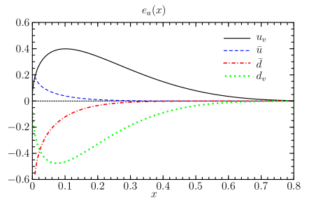
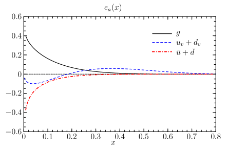
The parameters resulting from this modeling procedure are collected in Table 1, and the distributions at ξ=0𝜉0\xi=0 and t=0𝑡0t=0 for model 1 are shown in Fig. 2.

Table 1: Parameters in the ansatz (40) for different parton species a𝑎a in the two models described in the text. The values for valence quarks apply to both models, with normalization parameters given by kqv=κqN(αv,βqv)subscript𝑘subscript𝑞𝑣subscript𝜅𝑞𝑁subscript𝛼𝑣subscript𝛽subscript𝑞𝑣k_{q_{v}}=\kappa_{q}\mskip 1.5muN(\alpha_{v},\beta_{q_{v}}) according to (35). The last line gives the second Mellin moment at μ=2GeV𝜇2GeV\mu=2\operatorname{GeV} in the forward limit.
model 1 model 2
    uvsubscript𝑢𝑣u_{v}     dvsubscript𝑑𝑣d_{v}     u¯¯𝑢\bar{u}     d¯¯𝑑\bar{d}     g𝑔g     u¯¯𝑢\bar{u}     d¯¯𝑑\bar{d}     s¯¯𝑠\bar{s}     g𝑔g
αasubscript𝛼𝑎\alpha_{a} 0.550.55\phantom{-}0.55 0.550.55\phantom{-}0.55 1.251.25\phantom{-}1.25 1.251.25\phantom{-}1.25 1.101.10\phantom{-}1.10 1.251.25\phantom{-}1.25 1.251.25\phantom{-}1.25 1.251.25\phantom{-}1.25 1.101.10\phantom{-}1.10
βasubscript𝛽𝑎\beta_{a} 3.993.99\phantom{-}3.99 5.595.59\phantom{-}5.59 9.69.6\phantom{-}9.6 9.29.2\phantom{-}9.2 6.76.7\phantom{-}6.7 7.67.6\phantom{-}7.6 6.56.5\phantom{-}6.5 5.55.5\phantom{-}5.5 2.52.5\phantom{-}2.5
kasubscript𝑘𝑎k_{a} 1.711.71\phantom{-}1.71 2.362.36-2.36 0.060.06\phantom{-}0.06 0.180.18-0.18 0.260.26\phantom{-}0.26 0.00160.0016-0.0016 0.00180.0018-0.0018 0.00070.0007-0.0007 0.0170.017-0.017
01𝑑xxea(x)superscriptsubscript01differential-d𝑥𝑥subscript𝑒𝑎𝑥\int_{0}^{1}dx\,xe_{a}(x) 0.1380.138\phantom{-}0.138 0.1300.130-0.130 0.0130.013\phantom{-}0.013 0.0390.039-0.039 0.0440.044\phantom{-}0.044 0.00040.0004-0.0004 0.00050.0005-0.0005 0.00020.0002-0.0002 0.00590.0059-0.0059

We find that in model 2, both sea quark and gluon distributions are nearly zero (so that we do not attach importance to the unrealistically small value of βgsubscript𝛽𝑔\beta_{g} obtained with our above procedure). Their smallness can be traced back to the small value of the flavor singlet integral

01𝑑xx[euv(x)+edv(x)]=0.008superscriptsubscript01differential-d𝑥𝑥delimited-[]subscript𝑒subscript𝑢𝑣𝑥subscript𝑒subscript𝑑𝑣𝑥0.008\int_{0}^{1}dx\,x\bigl{[}e_{u_{v}}(x)+e_{d_{v}}(x)\bigr{]}=0.008 (47)

in the valence sector of our ansatz. In model 2, the distributions eq¯subscript𝑒¯𝑞e_{\bar{q}} and egsubscript𝑒𝑔e_{g} have the same sign as a consequence of (46) and due to the sum rule (3.1) can only be tiny. Somewhat larger distributions for sea quarks and gluons are obtained in model 1, where they have opposite sign because of (45).
Refer to caption
Refer to caption
Figure 2: The forward limits ea(x)subscript𝑒𝑎𝑥e_{a}(x) of the nucleon helicity-flip distributions at μ=2GeV𝜇2GeV\mu=2\operatorname{GeV} for different parton species a𝑎a in model 1.

We note that the parameters (3.1) we have taken for the valence part of Eqsuperscript𝐸𝑞E^{q} are by no means precisely determined by a fit to the Pauli form factors: alternative fits in [28] gave a similarly good description of the form factor data, with some variation of the resulting value of the integral in (47). Nevertheless, any model where euvsubscript𝑒subscript𝑢𝑣e_{u_{v}} and edvsubscript𝑒subscript𝑑𝑣e_{d_{v}} have similar shapes and no zeroes in x𝑥x will yield rather small values of this integral, given the strong cancellation between u𝑢u and d𝑑d quark contributions in the moment 01𝑑x[euv(x)+edv(x)]=κu+κd0.36superscriptsubscript01differential-d𝑥delimited-[]subscript𝑒subscript𝑢𝑣𝑥subscript𝑒subscript𝑑𝑣𝑥subscript𝜅𝑢subscript𝜅𝑑0.36\int_{0}^{1}dx\,\bigl{[}e_{u_{v}}(x)+e_{d_{v}}(x)\bigr{]}=\kappa_{u}+\kappa_{d}\approx-0.36. It would be interesting to explore how much the integral (47) and as a consequence the sea quark and gluon distributions can vary in realistic models, but such an investigation is beyond the scope of this work.

We end this section by quoting the values for the total angular momentum carried by quarks and antiquarks of a given flavor in our model, given by

Jq=1211𝑑xx[Hq(x,0,0)+Eq(x,0,0)]subscript𝐽𝑞12superscriptsubscript11differential-d𝑥𝑥delimited-[]superscript𝐻𝑞𝑥00superscript𝐸𝑞𝑥00J_{q}=\frac{1}{2}\int_{-1}^{1}dx\,x\bigl{[}H^{q}(x,0,0)+E^{q}(x,0,0)\bigr{]} (48)

according to Ji’s sum rule [2]. With the parameters in Table 1 and the CTEQ6M distributions we find

Jusubscript𝐽𝑢\displaystyle J_{u} =0.25,absent0.25\displaystyle=0.25\,, Jdsubscript𝐽𝑑\displaystyle J_{d} =0.01,absent0.01\displaystyle=-0.01\,, (model 1)
Jusubscript𝐽𝑢\displaystyle J_{u} =0.24,absent0.24\displaystyle=0.24\,, Jdsubscript𝐽𝑑\displaystyle J_{d} =0.03absent0.03\displaystyle=\phantom{-}0.03 (model 2) (49)

at the scale μ=2GeV𝜇2GeV\mu=2\operatorname{GeV} of our model. We note that this is in rather good agreement with the results of recent lattice calculations, with Ju=0.214(16)subscript𝐽𝑢0.21416J_{u}=0.214(16) and Jd=0.001(16)subscript𝐽𝑑0.00116J_{d}=-0.001(16) reported in [32], and Ju=0.33(2)subscript𝐽𝑢0.332J_{u}=0.33(2) and Jd=0.02(2)subscript𝐽𝑑0.022J_{d}=-0.02(2) in [33]. Let us reiterate that with just two sets of model parameters we cannot exhaust the range of possible scenarios but only provide two representatives that are consistent with presently known constraints. As just discussed, the relative smallness of sea quark and gluon distributions compared with the nucleon helicity conserving case should however be typical of a rather wide class of models.

4 Vector meson production at small xBsubscript𝑥𝐵x_{B}

We now study numerically the importance of NLO corrections in vector meson production. Here and in the following sections we use the two-loop strong coupling for nf=3subscript𝑛𝑓3n_{f}=3 flavors with a QCD scale parameter Λ(3)=226MeVsuperscriptΛ3226MeV\Lambda^{(3)}=226\operatorname{MeV}. This value corresponds to Λ(4)=326MeVsuperscriptΛ4326MeV\Lambda^{(4)}=326\operatorname{MeV}, Λ(5)=372MeVsuperscriptΛ5372MeV\Lambda^{(5)}=372\operatorname{MeV} and to αs(5)(MZ)=0.118superscriptsubscript𝛼𝑠5subscript𝑀𝑍0.118\alpha_{\smash{s}}^{(5)}(M_{Z})=0.118 when matching at mc=1.3GeVsubscript𝑚𝑐1.3GeVm_{c}=1.3\operatorname{GeV} and mb=4.5GeVsubscript𝑚𝑏4.5GeVm_{b}=4.5\operatorname{GeV}, which are the values used in the CTEQ6M parton analysis [29]. We also take nf=3subscript𝑛𝑓3n_{f}=3 fixed in the evolution and the hard-scattering kernels. Taking nf=4subscript𝑛𝑓4n_{f}=4 with massless charm or nf=5subscript𝑛𝑓5n_{f}=5 with massless charm and bottom would not be a good approximation for the rather moderate values of Q2superscript𝑄2Q^{2} we will discuss for fixed-target kinematics. On the other hand, taking nf=3subscript𝑛𝑓3n_{f}=3 and neglecting charm altogether is admittedly not a good approximation for the larger Q2superscript𝑄2Q^{2} relevant in collider kinematics. However, with αs(3)=0.164superscriptsubscript𝛼𝑠30.164\alpha_{\smash{s}}^{(3)}=0.164 compared to αs(5)=0.178superscriptsubscript𝛼𝑠50.178\alpha_{\smash{s}}^{(5)}=0.178 at μ=10GeV𝜇10GeV\mu=10\operatorname{GeV} we expect that this inaccuracy will not affect the conclusions at high Q2superscript𝑄2Q^{2} we shall draw from our studies.

We have performed the evolution of the GPDs at LO using the momentum-space evolution code of [34]. As explained in Sect. 2, taking LO evolution together with the NLO hard-scattering kernels is sufficient to obtain scale independence of the process amplitude up to uncalculated corrections of order αs3superscriptsubscript𝛼𝑠3\alpha_{s}^{3}. With the input scale of evolution not taken too small, NLO evolution effects should be rather moderate at the Q2superscript𝑄2Q^{2} values relevant in fixed-target kinematics, whereas our general conclusions for high Q2superscript𝑄2Q^{2} and small xBsubscript𝑥𝐵x_{B} will again not depend on this level of detail. We note that the NLO kernels in momentum space are available in the literature [35], but their considerable length makes it difficult to implement them in a fast numerical evaluation. For including NLO effects in the evolution it should be more efficient to use the Mellin space approach recently followed for deeply virtual Compton scattering in [5].

Here and in the following section we consider the convolutions of hard-scattering kernels with GPDs at t=0𝑡0t=0. For nonzero ξ=xB/(2xB)𝜉subscript𝑥𝐵2subscript𝑥𝐵\xi=x_{B}/(2-x_{B}) this should be understood in the sense of an analytic continuation, since the physical region for meson production is t4mp2ξ2/(1ξ2)𝑡4superscriptsubscript𝑚𝑝2superscript𝜉21superscript𝜉2-t\geq 4m_{p}^{2}\mskip 1.5mu\xi^{2}/(1-\xi^{2}) in Bjorken kinematics. To explore the importance of NLO corrections we do not see this as a shortcoming.
Refer to caption
Refer to caption
Refer to caption
Refer to caption
Refer to caption
Refer to caption
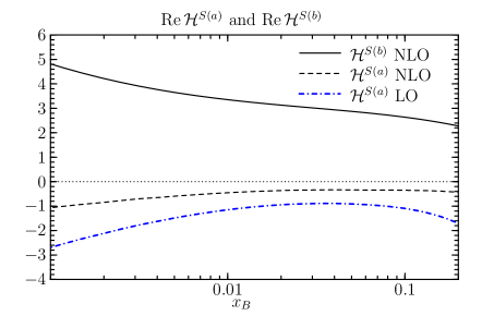
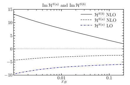
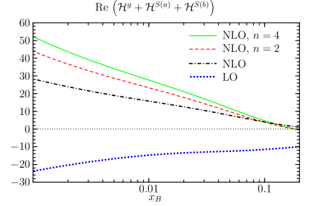
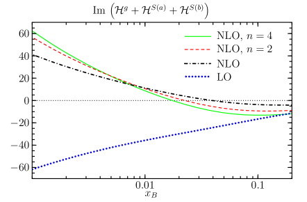
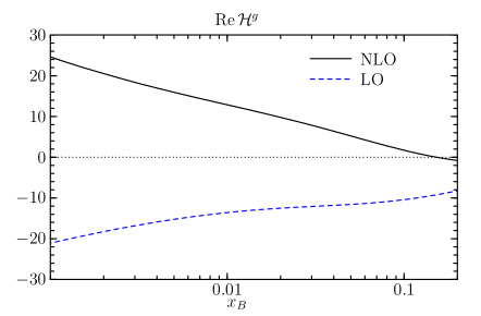
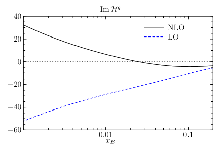
Figure 3: LO and NLO terms of the convolutions in the gluon and quark singlet sector at Q=4GeV𝑄4GeVQ=4\operatorname{GeV}. The scales are set to μR=μGPD=μDA=Qsubscript𝜇𝑅subscript𝜇𝐺𝑃𝐷subscript𝜇𝐷𝐴𝑄\mu_{R}=\mu_{GPD}=\mu_{DA}=Q. The NLO terms are for Gegenbauer index n=0𝑛0n=0 unless specified explicitly. Here and in the following plots the label “NLO” denotes the O(αs2)𝑂superscriptsubscript𝛼𝑠2O(\alpha_{s}^{2}) part of the convolutions, whereas the sum of O(αs)𝑂subscript𝛼𝑠O(\alpha_{s}) and O(αs2)𝑂superscriptsubscript𝛼𝑠2O(\alpha_{s}^{2}) terms is labeled by “LO+NLO”.
Refer to caption
Refer to caption
Refer to caption
Refer to caption
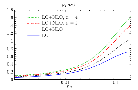
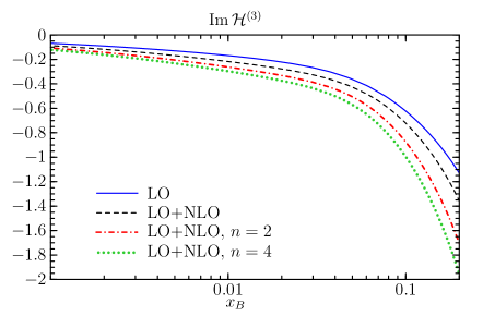
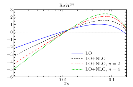
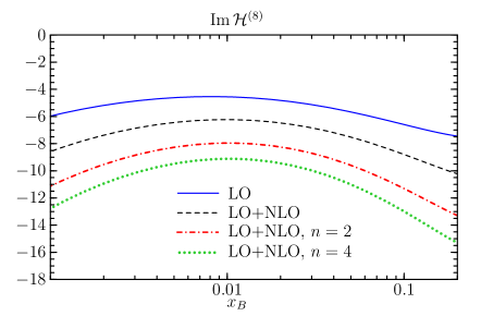
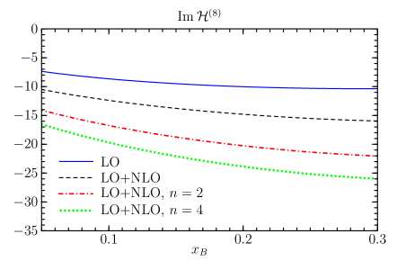
Figure 4: LO terms and the sum of LO and NLO terms of the convolutions in the quark non-singlet sector at Q=4GeV𝑄4GeVQ=4\operatorname{GeV}, with μR=μGPD=μDA=Qsubscript𝜇𝑅subscript𝜇𝐺𝑃𝐷subscript𝜇𝐷𝐴𝑄\mu_{R}=\mu_{GPD}=\mu_{DA}=Q.
Refer to caption
Refer to caption
Refer to caption
Refer to caption
Refer to caption
Refer to caption
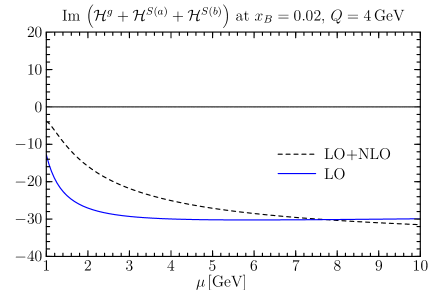
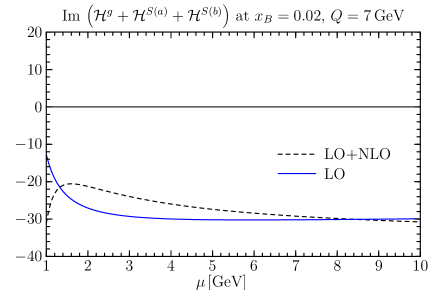
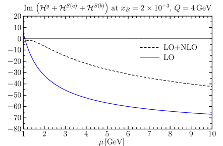
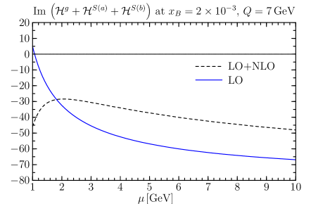
Figure 5: Dependence on the common scale μ=μR=μGPD𝜇subscript𝜇𝑅subscript𝜇𝐺𝑃𝐷\mu=\mu_{R}=\mu_{GPD} for the sum of convolutions in the gluon and quark singlet sector.

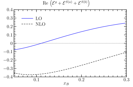
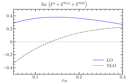
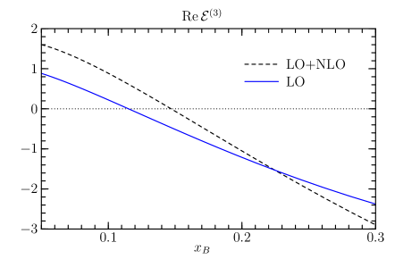
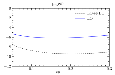
Let us start our discussion with the gluon and quark singlet sector. Here and in following we shall always present the convolutions (2.1) for Gegenbauer index n=0𝑛0n=0 unless indicated otherwise. In Fig. 3 we show the LO and NLO pieces of the convolutions for the scale choice μR=μGPD=μDA=Qsubscript𝜇𝑅subscript𝜇𝐺𝑃𝐷subscript𝜇𝐷𝐴𝑄\mu_{R}=\mu_{GPD}=\mu_{DA}=Q. The size of corrections at small xBsubscript𝑥𝐵x_{B} is dramatic: we have large NLO corrections with opposite sign compared to the LO term for gsuperscript𝑔\mathcal{H}^{g}, and a similarly large NLO contribution from S(b)superscript𝑆𝑏\mathcal{H}^{S(b)} with sign opposite to the LO result for S(a)superscript𝑆𝑎\mathcal{H}^{S(a)}. In the sum of gluon and quark singlet terms, the NLO corrections drastically reduce the LO result or even lead to a change of sign between LO and the sum of LO and NLO results. We also observe that for higher Gegenbauer index the NLO corrections tend to be even more important. Note that the LO term of the convolutions is the same for all n𝑛n as can be seen from (2.1) and (2.1). The size of NLO corrections in S(a)superscript𝑆𝑎\mathcal{H}^{S(a)} is comparatively moderate, at least for lower Gegenbauer moments. The same is seen for the quark non-singlet convolutions in Fig. 4. Of course, the gluon and quark singlet terms will dominate meson production at small xBsubscript𝑥𝐵x_{B} in those channels where it is allowed by the meson quantum numbers.

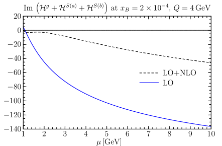
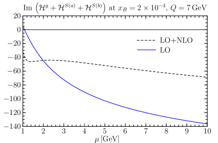
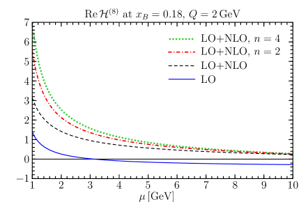
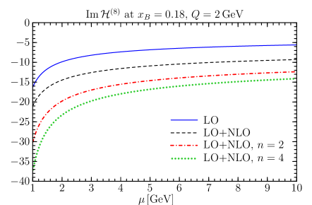
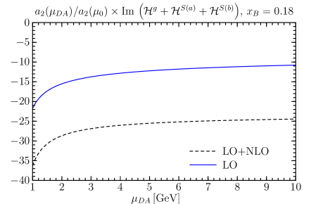
In Fig. 5 we explore the influence of the scale choice by varying μR=μGPDsubscript𝜇𝑅subscript𝜇𝐺𝑃𝐷\mu_{R}=\mu_{GPD} simultaneously. For xB=2×10³subscript𝑥𝐵2superscript103x_{B}=2\times 10^{-3} we find an indication for the onset of perturbative stability at Q=7GeV𝑄7GeVQ=7\operatorname{GeV} but not yet at Q=4GeV𝑄4GeVQ=4\operatorname{GeV}. For xB=2×10²subscript𝑥𝐵2superscript102x_{B}=2\times 10^{-2} the situation is less severe, with moderate corrections in a wide μ𝜇\mu range already at Q=4GeV𝑄4GeVQ=4\operatorname{GeV}. In contrast, when going down to xB=2×10⁴subscript𝑥𝐵2superscript104x_{B}=2\times 10^{-4} we find very large corrections even at Q=7GeV𝑄7GeVQ=7\operatorname{GeV}. We have checked that the conclusions in the respective kinematics do not change when we vary μGPDsubscript𝜇𝐺𝑃𝐷\mu_{GPD} while keeping μR=Qsubscript𝜇𝑅𝑄\mu_{R}=Q fixed.

Refer to caption
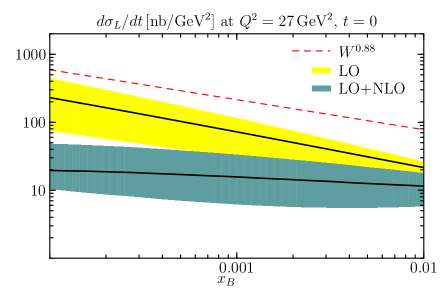
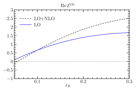
Figure 6: Cross section for γpρpsuperscript𝛾𝑝𝜌𝑝\gamma^{*}p\to\rho\mskip 1.5mup with longitudinal photon polarization. Bands correspond to the range Q/2<μ<2Q𝑄2𝜇2𝑄Q/2<\mu<2Q and solid lines to μ=Q𝜇𝑄\mu=Q. We also show the power-law behavior σW0.88proportional-to𝜎superscript𝑊0.88\sigma\propto W^{0.88} (with arbitrary normalization) obtained from a fit to data in the range 0.001<xB<0.005superscriptsimilar-to0.001subscript𝑥𝐵superscriptsimilar-to0.0050.001\raisebox{-4.0pt}{$\,\stackrel{{\scriptstyle\textstyle<}}{{\sim}}\,$}x_{B}\raisebox{-4.0pt}{$\,\stackrel{{\scriptstyle\textstyle<}}{{\sim}}\,$}0.005 [36].

Figure 6 shows how the perturbative instability we observed in the convolutions affects the longitudinal cross section for ρ𝜌\rho production. Here we have taken the asymptotic form of the meson distribution amplitude, i.e. set an=0subscript𝑎𝑛0a_{n}=0 for n2𝑛2n\geq 2. In the NLO result for the cross section we have squared the coherent sum of LO and NLO terms in the process amplitude,222We thus keep terms of O(αs3)𝑂superscriptsubscript𝛼𝑠3O(\alpha_{s}^{3}) in the cross section, although the accuracy of the NLO calculation is only up to O(αs2)𝑂superscriptsubscript𝛼𝑠2O(\alpha_{s}^{2}). This should not be seen as a problem, as it will not make a considerable difference in situations where perturbative corrections are moderate, whereas in situations where NLO corrections are huge we would neither trust the cross section with or without the partially included O(αs3)𝑂superscriptsubscript𝛼𝑠3O(\alpha_{s}^{3}) terms. i.e. we have taken |LO+NLO|2superscriptsubscriptLOsubscriptNLO2|\mathcal{M}_{\mathrm{LO}}+\mathcal{M}_{\mathrm{NLO}}|^{2}. We see that the NLO corrections severely decrease the LO result. As a consequence of the cancellations between LO and NLO contributions, the scale dependence of the cross section does not decrease. We also show in the figure the power-law behavior σW0.88proportional-to𝜎superscript𝑊0.88\sigma\propto W^{0.88} obtained from a fit to data in the range 0.001<xB<0.005superscriptsimilar-to0.001subscript𝑥𝐵superscriptsimilar-to0.0050.001\raisebox{-4.0pt}{$\,\stackrel{{\scriptstyle\textstyle<}}{{\sim}}\,$}x_{B}\raisebox{-4.0pt}{$\,\stackrel{{\scriptstyle\textstyle<}}{{\sim}}\,$}0.005 [36]. As observed in [13], a double distribution model with the CTEQ6M distributions as input lead to a rather good description of this experimentally observed energy dependence if the cross section is evaluated at LO. With the strong cancellations from the O(αs2)𝑂superscriptsubscript𝛼𝑠2O(\alpha_{s}^{2}) corrections, one obtains an NLO result whose energy behavior is much too weak.
Refer to caption
Refer to caption
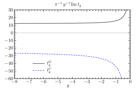
Figure 7: The factorization scale dependent and independent terms of Imtg,nImsubscript𝑡𝑔𝑛\operatorname{Im}t_{g,n} and Imtb,nImsubscript𝑡𝑏𝑛\operatorname{Im}t_{b,n} as specified in (4), shown for n=0𝑛0n=0 and y<0𝑦0y<0.

Let us discuss how the huge size of corrections can be understood at an analytical level, following the line of argument given in [11, 37]. Using (81) and (82) we can approximate the hard-scattering kernels for large negative y𝑦y as

1πImg(z,y)1𝜋Imsubscript𝑔𝑧𝑦\displaystyle\frac{1}{\pi}\,\operatorname{Im}\mathcal{I}_{g}(z,y) =4CA[ln(zz¯)+lnQ2μGPD2]y+O(1),absent4subscript𝐶𝐴delimited-[]𝑧¯𝑧superscript𝑄2superscriptsubscript𝜇𝐺𝑃𝐷2𝑦𝑂1\displaystyle=4C_{A}\biggl{[}\ln(z\bar{z})+\ln\frac{Q^{2}}{\mu_{GPD}^{2}}\biggr{]}\mskip 1.5muy+O(1)\,, Reg(z,y)Resubscript𝑔𝑧𝑦\displaystyle\operatorname{Re}\mathcal{I}_{g}(z,y) =O(1),absent𝑂1\displaystyle=O(1)\,,
1πImb(z,y)1𝜋Imsubscript𝑏𝑧𝑦\displaystyle\frac{1}{\pi}\operatorname{Im}\mathcal{I}_{b}(z,y) =4[1ln(zz¯)lnQ2μGPD2]+O(y1),absent4delimited-[]1𝑧¯𝑧superscript𝑄2superscriptsubscript𝜇𝐺𝑃𝐷2𝑂superscript𝑦1\displaystyle=4\biggl{[}1-\ln(z\bar{z})-\ln\frac{Q^{2}}{\mu_{GPD}^{2}}\biggr{]}+O\bigl{(}y^{-1}\bigr{)}\,, Reb(z,y)Resubscript𝑏𝑧𝑦\displaystyle\operatorname{Re}\mathcal{I}_{b}(z,y) =O(y1),absent𝑂superscript𝑦1\displaystyle=O\bigl{(}y^{-1}\bigr{)}\,, (50)

where here and in the following the order of corrections is given up to powers of lny¯¯𝑦\ln\bar{y}. The quark non-singlet kernel is subleading compared with the pure singlet one,

a(z¯,y)ya(z,y¯)y¯O(y1),similar-tosubscript𝑎¯𝑧𝑦𝑦subscript𝑎𝑧¯𝑦¯𝑦similar-to𝑂superscript𝑦1\displaystyle\frac{\mathcal{I}_{a}(\bar{z},y)}{y}\sim\frac{\mathcal{I}_{a}(z,\bar{y})}{\bar{y}}\sim O\bigl{(}y^{-1}\bigr{)}\,, (51)

where we have divided a(z¯,y)subscript𝑎¯𝑧𝑦\mathcal{I}_{a}(\bar{z},y) by y𝑦y corresponding to the prefactor in the complete kernel (2). From (4) we readily obtain

1πImtg,n(y)1𝜋Imsubscript𝑡𝑔𝑛𝑦\displaystyle\frac{1}{\pi}\operatorname{Im}t_{g,n}(y) =4CA[cnlnQ2μGPD2]y+O(1),absent4subscript𝐶𝐴delimited-[]subscript𝑐𝑛superscript𝑄2subscriptsuperscript𝜇2𝐺𝑃𝐷𝑦𝑂1\displaystyle=-4C_{A}\biggl{[}c_{n}-\ln\frac{Q^{2}}{\mu^{2}_{GPD}}\biggr{]}\mskip 1.5muy+O(1)\,,
1πImtb,n(y)1𝜋Imsubscript𝑡𝑏𝑛𝑦\displaystyle\frac{1}{\pi}\operatorname{Im}t_{b,n}(y) =4[cn+1lnQ2μGPD2]+O(y1)absent4delimited-[]subscript𝑐𝑛1superscript𝑄2subscriptsuperscript𝜇2𝐺𝑃𝐷𝑂superscript𝑦1\displaystyle=4\biggl{[}c_{n}+1-\ln\frac{Q^{2}}{\mu^{2}_{GPD}}\biggr{]}+O\bigl{(}y^{-1}\bigr{)} (52)

with constants

c0subscript𝑐0\displaystyle c_{0} =2,absent2\displaystyle=2\,, c2subscript𝑐2\displaystyle c_{2} =1133.7,absent1133.7\displaystyle=\frac{11}{3}\approx 3.7\,, c4subscript𝑐4\displaystyle c_{4} =137304.6,absent137304.6\displaystyle=\frac{137}{30}\approx 4.6\,, cnsubscript𝑐𝑛\displaystyle c_{n} =01𝑑zln(zz¯)Cn3/2(2z1)absentsuperscriptsubscript01differential-d𝑧𝑧¯𝑧superscriptsubscript𝐶𝑛322𝑧1\displaystyle=-\int_{0}^{1}dz\,\ln(z\bar{z})\,C_{n}^{3/2}(2z-1) (53)

that increase with the Gegenbauer index n𝑛n. In Fig. 7 we show for the case n=0𝑛0n=0 that these approximations become very good for increasing |y|𝑦|y|, where we have decomposed the exact kernels as

Imtg,n(y)Imsubscript𝑡𝑔𝑛𝑦\displaystyle\operatorname{Im}t_{g,n}(y) =Imtg,nC(y)+Imtg,nG(y)lnQ2μGPD2,absentImsuperscriptsubscript𝑡𝑔𝑛𝐶𝑦Imsuperscriptsubscript𝑡𝑔𝑛𝐺𝑦superscript𝑄2subscriptsuperscript𝜇2𝐺𝑃𝐷\displaystyle=\operatorname{Im}t_{g,n}^{C}(y)+\operatorname{Im}t_{g,n}^{G}(y)\mskip 1.5mu\ln\frac{Q^{2}}{\mu^{2}_{GPD}}\,,
Imtb,n(y)Imsubscript𝑡𝑏𝑛𝑦\displaystyle\operatorname{Im}t_{b,n}(y) =Imtb,nC(y)+Imtb,nG(y)lnQ2μGPD2.absentImsuperscriptsubscript𝑡𝑏𝑛𝐶𝑦Imsuperscriptsubscript𝑡𝑏𝑛𝐺𝑦superscript𝑄2subscriptsuperscript𝜇2𝐺𝑃𝐷\displaystyle=\operatorname{Im}t_{b,n}^{C}(y)+\operatorname{Im}t_{b,n}^{G}(y)\mskip 1.5mu\ln\frac{Q^{2}}{\mu^{2}_{GPD}}\,. (54)

Let us now rewrite the convolutions of kernels and GPDs in terms of the variable ω=x/ξ𝜔𝑥𝜉\omega=x/\xi,

Im[ng+nS(b)]=6αs[πHg(ξ,ξ,t)+αs4πIm01/ξdω\displaystyle\operatorname{Im}\mskip 1.5mu\Bigl{[}\mathcal{H}^{g}_{n}+\mathcal{H}^{S(b)}_{n}\Bigr{]}=-6\alpha_{s}\,\biggl{[}\pi H^{g}(\xi,\xi,t)+\frac{\alpha_{s}}{4\pi}\operatorname{Im}\int_{0}^{1/\xi}d\omega
×{21ωiϵtg,n(1ωiϵ2)Hg(ωξ,ξ,t)1+ωCFtb,n(1ωiϵ2)ξHS(ωξ,ξ,t)}].\displaystyle\qquad\times\biggl{\{}\frac{2}{1-\omega-i\epsilon}\;t_{g,n}\biggl{(}\frac{1-\omega-i\epsilon}{2}\biggr{)}\,\frac{H^{g}(\omega\xi,\xi,t)}{1+\omega}-C_{F}\,t_{b,n}\biggl{(}\frac{1-\omega-i\epsilon}{2}\biggr{)}\,\xi H^{S}(\omega\xi,\xi,t)\biggr{\}}\biggr{]}\,. (55)

For ωω0𝜔subscript𝜔0\omega\geq\omega_{0} with some ω01much-greater-thansubscript𝜔01\omega_{0}\gg 1 we can use the approximation (4) of the hard-scattering kernels, and further approximate 1+ωω1𝜔𝜔1+\omega\approx\omega in the first term on the second line. This gives

16παsIm[ng+nS(b)]Hg(ξ,ξ,t)+αsπ0ω0𝑑ω16𝜋subscript𝛼𝑠Imsubscriptsuperscript𝑔𝑛subscriptsuperscript𝑆𝑏𝑛superscript𝐻𝑔𝜉𝜉𝑡subscript𝛼𝑠𝜋superscriptsubscript0subscript𝜔0differential-d𝜔\displaystyle-\frac{1}{6\pi\alpha_{s}}\operatorname{Im}\mskip 1.5mu\Bigl{[}\mathcal{H}^{g}_{n}+\mathcal{H}^{S(b)}_{n}\Bigr{]}\,\approx\,H^{g}(\xi,\xi,t)+\frac{\alpha_{s}}{\pi}\,\int_{0}^{\omega_{0}}d\omega\,\ldots
αsπω01/ξ𝑑ω{CA[cnlnQ2μGPD2]Hg(ωξ,ξ,t)ω+CF[cn+1lnQ2μGPD2]ξHS(ωξ,ξ,t)},subscript𝛼𝑠𝜋superscriptsubscriptsubscript𝜔01𝜉differential-d𝜔subscript𝐶𝐴delimited-[]subscript𝑐𝑛superscript𝑄2subscriptsuperscript𝜇2𝐺𝑃𝐷superscript𝐻𝑔𝜔𝜉𝜉𝑡𝜔subscript𝐶𝐹delimited-[]subscript𝑐𝑛1superscript𝑄2subscriptsuperscript𝜇2𝐺𝑃𝐷𝜉superscript𝐻𝑆𝜔𝜉𝜉𝑡\displaystyle-\frac{\alpha_{s}}{\pi}\,\int_{\omega_{0}}^{1/\xi}d\omega\,\biggl{\{}C_{A}\biggl{[}c_{n}-\ln\frac{Q^{2}}{\mu^{2}_{GPD}}\biggr{]}\,\frac{H^{g}(\omega\xi,\xi,t)}{\omega}+C_{F}\biggl{[}c_{n}+1-\ln\frac{Q^{2}}{\mu^{2}_{GPD}}\biggr{]}\,\xi H^{S}(\omega\xi,\xi,t)\biggr{\}}\,, (56)

where the integral over ω𝜔\omega on the first line is to be taken with the unapproximated integrand from (4). It grows with ξ𝜉\xi like Hg(ωξ,ξ,t)superscript𝐻𝑔𝜔𝜉𝜉𝑡H^{g}(\omega\xi,\xi,t) or ξHS(ωξ,ξ,t)𝜉superscript𝐻𝑆𝜔𝜉𝜉𝑡\xi H^{S}(\omega\xi,\xi,t) but lacks the enhancement due to the upper limit 1/ξ1𝜉1/\xi of the integral on the second line. Restricting our discussion to t=0𝑡0t=0 for simplicity, we can for sufficiently large ω𝜔\omega neglect the effect of skewness in the GPDs and then have

Hg(ωξ,ξ,0)superscript𝐻𝑔𝜔𝜉𝜉0\displaystyle H^{g}(\omega\xi,\xi,0) ωξg(ωξ),absent𝜔𝜉𝑔𝜔𝜉\displaystyle\approx\omega\xi\mskip 1.5mug(\omega\xi)\,, HS(ωξ,ξ,0)superscript𝐻𝑆𝜔𝜉𝜉0\displaystyle H^{S}(\omega\xi,\xi,0) S(ωξ)=q[q(ωξ)+q¯(ωξ)],absent𝑆𝜔𝜉subscript𝑞delimited-[]𝑞𝜔𝜉¯𝑞𝜔𝜉\displaystyle\approx S(\omega\xi)=\sum\nolimits_{q}\,\bigl{[}q(\omega\xi)+\bar{q}(\omega\xi)\bigr{]}\,, (57)

where S(x)𝑆𝑥S(x) is the usual quark singlet distribution. In a very rough approximation one may treat xg(x)𝑥𝑔𝑥xg(x) and xS(x)𝑥𝑆𝑥xS(x) as constant at small x𝑥x. In (4) one then has loop integrals 𝑑ω/ωdifferential-d𝜔𝜔\int d\omega/\omega for both the gluon and the quark term, which generate large logarithms ln(ω0ξ)subscript𝜔0𝜉\ln(\omega_{0}\mskip 1.5mu\xi) for 1/ξω0much-greater-than1𝜉subscript𝜔01/\xi\gg\omega_{0}. These logarithms are of BFKL type and correspond to graphs with t𝑡t-channel gluon exchange in the hard-scattering kernel, such as those for Tbsubscript𝑇𝑏T_{b} and Tgsubscript𝑇𝑔T_{g} in Fig. 1.

In a phenomenologically more realistic approximation one has xg(x)axλ𝑥𝑔𝑥𝑎superscript𝑥𝜆xg(x)\approx a\mskip 1.5mux^{-\lambda} at small x𝑥x and a similar behavior with different values of a𝑎a and λ𝜆\lambda for xS(x)𝑥𝑆𝑥xS(x). This gives

ω01/ξ𝑑ωHg(ωξ,ξ,0)ωaξλω01/ξ𝑑ωωλ1aλ(ω0ξ)λsuperscriptsubscriptsubscript𝜔01𝜉differential-d𝜔superscript𝐻𝑔𝜔𝜉𝜉0𝜔𝑎superscript𝜉𝜆superscriptsubscriptsubscript𝜔01𝜉differential-d𝜔superscript𝜔𝜆1𝑎𝜆superscriptsubscript𝜔0𝜉𝜆\int_{\omega_{0}}^{1/\xi}d\omega\,\frac{H^{g}(\omega\xi,\xi,0)}{\omega}\approx a\mskip 1.5mu\xi^{-\lambda}\int_{\omega_{0}}^{1/\xi}d\omega\,\omega^{-\lambda-1}\approx\frac{a}{\lambda}\,\bigl{(}\omega_{0}\mskip 1.5mu\xi\bigr{)}^{-\lambda} (58)

for 1/ξω0much-greater-than1𝜉subscript𝜔01/\xi\gg\omega_{0}, when the bulk of the integral comes from the region where the small-x𝑥x approximation of the gluon density is valid. With λ𝜆\lambda being rather small for the gluon distribution in a wide range of the factorization scale, the term (58) has the same power behavior ξλsuperscript𝜉𝜆\xi^{-\lambda} as the Born term Hg(ξ,ξ,0)superscript𝐻𝑔𝜉𝜉0H^{g}(\xi,\xi,0) in (4) but is numerically enhanced by 1/λ1𝜆1/\lambda. A contribution analogous to (58) is obtained from the quark singlet term in (4) and comes with a similar enhancement.

Concerning the choice of factorization scale, it is clear that the size of the corrections in (4) is decreased if μGPDsubscript𝜇𝐺𝑃𝐷\mu_{GPD} is taken smaller than Q𝑄Q. It is also clear that no scale choice can eliminate both the gluon and quark singlet contribution in this expression. To make at least the gluon term for n=0𝑛0n=0 disappear one needs μGPD2=e2Q20.14Q2superscriptsubscript𝜇𝐺𝑃𝐷2superscript𝑒2superscript𝑄20.14superscript𝑄2\mu_{GPD}^{2}=e^{-2}\mskip 1.5muQ^{2}\approx 0.14\,Q^{2}. For a wide range of Q2superscript𝑄2Q^{2} this is outside the perturbative region or at least so low that the quark singlet distribution has a rather small power λ𝜆\lambda and can thus give important corrections. We note that previous analyses of vector meson production at small xBsubscript𝑥𝐵x_{B} have argued for a factorization scale well below Q2superscript𝑄2Q^{2}, based on different estimates of the typical virtualities in the leading-order graphs [15, 38]. We also note that the μRsubscript𝜇𝑅\mu_{R} dependent term β0ln(μR2/μGPD2)subscript𝛽0superscriptsubscript𝜇𝑅2subscriptsuperscript𝜇2𝐺𝑃𝐷\beta_{0}\ln(\mu_{R}^{2}/\mu^{2}_{GPD}) in the gluon kernel (2) does not appear in the approximation (4) which dominates the convolutions at small xBsubscript𝑥𝐵x_{B}. The choice of μRsubscript𝜇𝑅\mu_{R} can thus not cure the huge NLO corrections we have discussed.

5 Vector meson production at moderate to large xBsubscript𝑥𝐵x_{B}

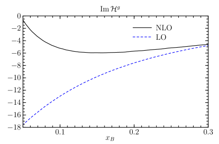
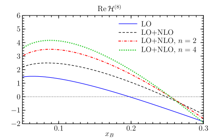
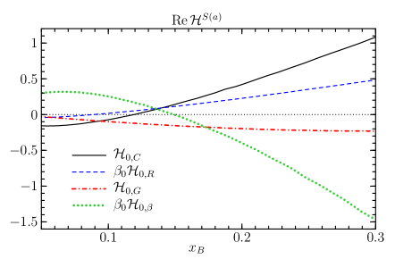
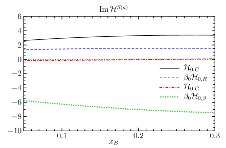
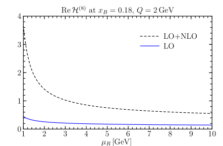
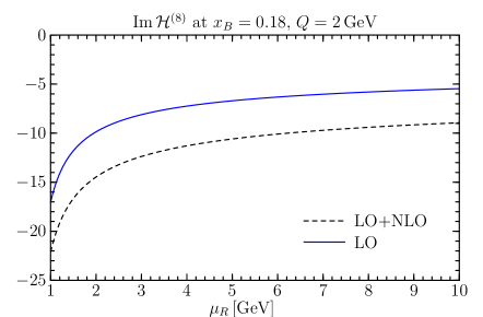
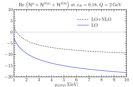
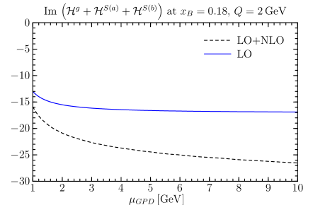
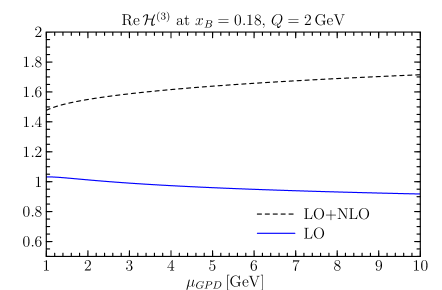
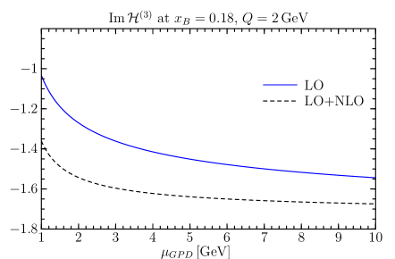
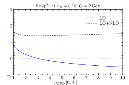
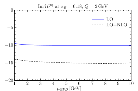
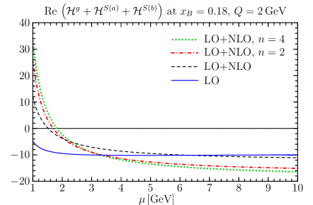
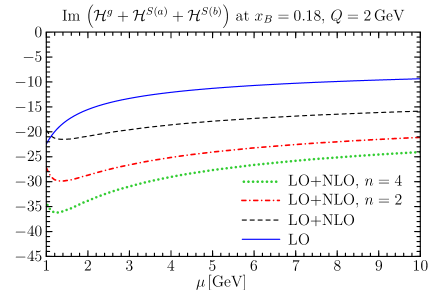
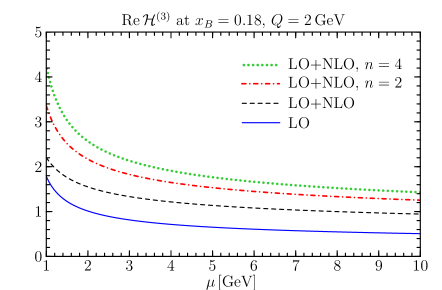
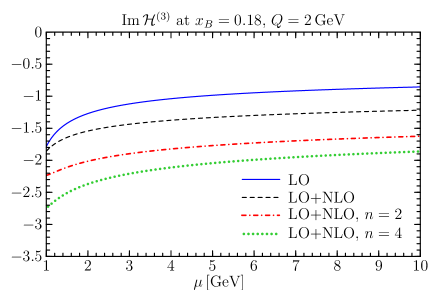
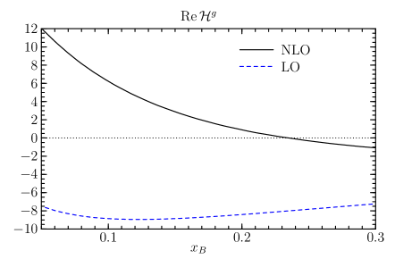
Let us now investigate the NLO corrections in typical fixed-target kinematics, as it is accessible at HERMES, JLab and COMPASS. We take again t=0𝑡0t=0 and for definiteness present estimates at Q2=4GeV2superscript𝑄24superscriptGeV2Q^{2}=4\operatorname{GeV}^{2}. For larger Q2superscript𝑄2Q^{2}, which will in particular be accessible with the JLab energy upgrade to 12GeV12GeV12\operatorname{GeV}, the corrections are in general smaller.
Refer to caption
Refer to caption
Refer to caption
Refer to caption
Refer to caption
Refer to caption
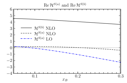
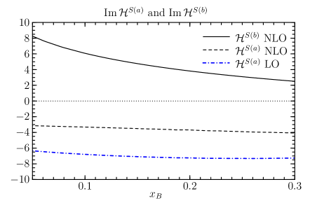
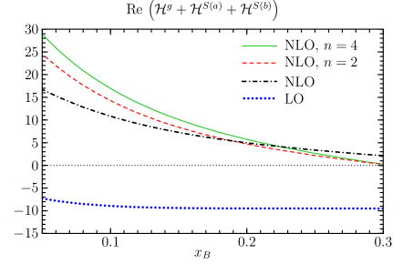
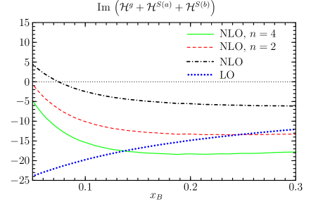
Figure 8: LO and NLO terms of the convolutions in the gluon and quark singlet sector at Q=2GeV𝑄2GeVQ=2\operatorname{GeV}, with μR=μGPD=μDA=Qsubscript𝜇𝑅subscript𝜇𝐺𝑃𝐷subscript𝜇𝐷𝐴𝑄\mu_{R}=\mu_{GPD}=\mu_{DA}=Q.

In Fig. 8 we compare the LO and NLO parts of the convolution integrals. In the gluon sector we find no simple picture, with relative corrections that are typically moderate but become large for RegResuperscript𝑔\operatorname{Re}\mathcal{H}^{g} at smaller xBsubscript𝑥𝐵x_{B} and for ImgImsuperscript𝑔\operatorname{Im}\mathcal{H}^{g} at larger xBsubscript𝑥𝐵x_{B}. For the quark singlet the situation is similar to the one in the small-xBsubscript𝑥𝐵x_{B} region, i.e. we have rather large NLO corrections from S(b)superscript𝑆𝑏\mathcal{H}^{S(b)} with sign opposite to the LO part of S(a)superscript𝑆𝑎\mathcal{H}^{S(a)}, whereas the NLO corrections in S(a)superscript𝑆𝑎\mathcal{H}^{S(a)} are smaller. Adding gluon and quark singlet contributions, we find that for n=0𝑛0n=0 the NLO corrections are of reasonable size for the imaginary part. For the real part at lower xBsubscript𝑥𝐵x_{B}, the corrections are however large and of opposite sign compared to the Born term. We note that the convolutions \mathcal{H} satisfy a dispersion relation in 1/xB1subscript𝑥𝐵1/x_{B} for fixed Q2superscript𝑄2Q^{2} and t𝑡t [39]. In this representation their real parts at a given xBsubscript𝑥𝐵x_{B} are sensitive to the imaginary part at smaller values of xBsubscript𝑥𝐵x_{B}, where the NLO corrections rapidly increase as we have seen in the previous section. Turning to the quark non-singlet convolutions, we see in Fig. 9 that for n=0𝑛0n=0 the NLO corrections are comparatively moderate for the imaginary part and larger for the real part.

Going from n=0𝑛0n=0 to higher Gegenbauer indices n=2𝑛2n=2 and n=4𝑛4n=4, the NLO corrections become larger, as we see in Figs. 8 and 9 and already observed at small xBsubscript𝑥𝐵x_{B}. Generically this is not unexpected, since the z𝑧z dependent kernels (2) contain logarithms lnz𝑧\ln z and lnz¯¯𝑧\ln\bar{z} which enhance the endpoint regions of the z𝑧z integration, and those endpoint regions are more prominent for higher Gegenbauer polynomials in the expansion (15). Note that according to phenomenological estimates or lattice calculations the coefficients ansubscript𝑎𝑛a_{n} of these polynomials are clearly smaller than a0subscript𝑎0a_{0}, so that increasing corrections to nsubscript𝑛\mathcal{H}_{n} for higher n𝑛n do not affect the sum nannsubscript𝑛subscript𝑎𝑛subscript𝑛\sum_{n}a_{n}\mathcal{H}_{n} as much. We note that in the modified hard-scattering approach of Sterman et al. [14], which goes beyond the collinear approximation used in the present work, the endpoint regions in z𝑧z are suppressed by radiative corrections that are resummed into Sudakov form factors. As just discussed, we do not observe such a suppression in the fixed-order results analyzed here, where various positive and negative corrections compete with each other—only some of them related to the Sudakov factor. How the situation will be at higher orders is an important question, which goes beyond the scope of the present work.
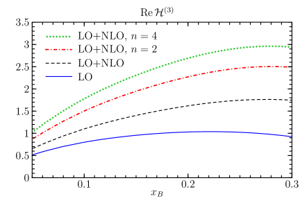
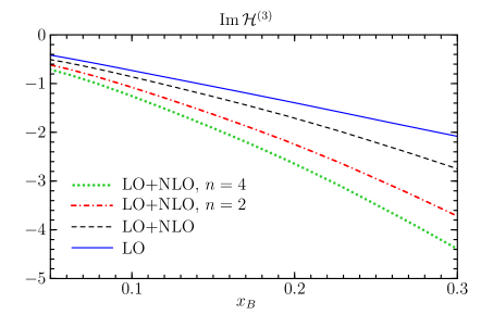
Refer to caption
Refer to caption
Refer to caption
Refer to caption
Figure 9: LO terms and the sum of LO and NLO terms of the convolutions in the quark non-singlet sector at Q=2GeV𝑄2GeVQ=2\operatorname{GeV}, with μR=μGPD=μDA=Qsubscript𝜇𝑅subscript𝜇𝐺𝑃𝐷subscript𝜇𝐷𝐴𝑄\mu_{R}=\mu_{GPD}=\mu_{DA}=Q.

Let us now take a closer look at the μRsubscript𝜇𝑅\mu_{R} dependence of the corrections. As we explained in Sect. 2, the pure quark singlet kernel Tbsubscript𝑇𝑏T_{b} is independent of this scale at O(αs2)𝑂superscriptsubscript𝛼𝑠2O(\alpha_{s}^{2}). According to (2) the gluon kernel Tgsubscript𝑇𝑔T_{g} depends on μR2superscriptsubscript𝜇𝑅2\mu_{R}^{2} only through β0ln(μR2/μGPD2)subscript𝛽0superscriptsubscript𝜇𝑅2subscriptsuperscript𝜇2𝐺𝑃𝐷\beta_{0}\ln(\mu_{R}^{2}/\mu^{2}_{GPD}), which originates from graphs with gluon propagator corrections such as the one shown in Fig. 10. The μGPDsubscript𝜇𝐺𝑃𝐷\mu_{GPD} dependence of this term is connected with the contribution proportional to β0subscript𝛽0\beta_{0} in the evolution kernel Vggsuperscript𝑉𝑔𝑔V^{gg} for the gluon GPD, given in (C). As already pointed out in Sect. 4, the term β0ln(μR2/μGPD2)subscript𝛽0superscriptsubscript𝜇𝑅2subscriptsuperscript𝜇2𝐺𝑃𝐷\beta_{0}\ln(\mu_{R}^{2}/\mu^{2}_{GPD}) does not contribute to the large-|y|𝑦|y| behavior of Imtg,n(y)Imsubscript𝑡𝑔𝑛𝑦\operatorname{Im}t_{g,n}(y) and is hence not relevant for the huge NLO corrections at small xBsubscript𝑥𝐵x_{B}.

Refer to caption
Figure 10: Example graphs giving rise to terms proportional to β0subscript𝛽0\beta_{0} in the hard-scattering kernels Tasubscript𝑇𝑎T_{a} and Tgsubscript𝑇𝑔T_{g}.

For the kernel Tasubscript𝑇𝑎T_{a} the situation is more involved. The general structure of its convolution with the quark singlet distribution HSsuperscript𝐻𝑆H^{S} can be written as

nS(a)subscriptsuperscript𝑆𝑎𝑛\displaystyle\mathcal{H}^{S(a)}_{n\phantom{P}} =β0(n,βS(a)+n,RS(a)lnQ2μR2)+n,CS(a)+n,GS(a)lnQ2μGPD2+n,DS(a)lnQ2μDA2absentsubscript𝛽0subscriptsuperscript𝑆𝑎𝑛𝛽subscriptsuperscript𝑆𝑎𝑛𝑅superscript𝑄2subscriptsuperscript𝜇2𝑅subscriptsuperscript𝑆𝑎𝑛𝐶subscriptsuperscript𝑆𝑎𝑛𝐺superscript𝑄2subscriptsuperscript𝜇2𝐺𝑃𝐷subscriptsuperscript𝑆𝑎𝑛𝐷superscript𝑄2subscriptsuperscript𝜇2𝐷𝐴\displaystyle=\beta_{0}\,\biggl{(}\mathcal{H}^{S(a)}_{n,\beta}+\mathcal{H}^{S(a)}_{n,R}\,\ln\frac{Q^{2}}{\mu^{2}_{R}}\biggr{)}+\mathcal{H}^{S(a)}_{n,C}+\mathcal{H}^{S(a)}_{n,G}\ln\frac{Q^{2}}{\mu^{2}_{GPD}}+\mathcal{H}^{S(a)}_{n,D}\ln\frac{Q^{2}}{\mu^{2}_{DA}} (59)

with an analogous decomposition for the convolutions n(3)subscriptsuperscript3𝑛\mathcal{H}^{(3)}_{n} and n(8)subscriptsuperscript8𝑛\mathcal{H}^{(8)}_{n}. The terms proportional to β0subscript𝛽0\beta_{0} originate from graphs with gluon propagator corrections such as in Fig. 10, whereas the terms with subscripts C,G,D𝐶𝐺𝐷C,G,D do not contain β0subscript𝛽0\beta_{0}. In Fig. 11 we show the corresponding contributions for n=0𝑛0n=0. We see that terms multiplying ln(Q2/μGPD2)superscript𝑄2subscriptsuperscript𝜇2𝐺𝑃𝐷\ln(Q^{2}/\mu^{2}_{GPD}) are rather small, whereas those going with ln(Q2/μDA2)superscript𝑄2subscriptsuperscript𝜇2𝐷𝐴\ln(Q^{2}/\mu^{2}_{DA}) are of course absent for n=0𝑛0n=0. The term 0,Rsubscript0𝑅\mathcal{H}_{0,R} is clearly smaller than 0,βsubscript0𝛽\mathcal{H}_{0,\beta} and has opposite sign. 0,Csubscript0𝐶\mathcal{H}_{0,C} has also the opposite sign compared to 0,βsubscript0𝛽\mathcal{H}_{0,\beta} but is similar in magnitude. We note that |n,β|subscript𝑛𝛽|\mathcal{H}_{n,\beta}| increases with n𝑛n, as can be seen from (B) and (B).

Refer to caption
Refer to caption
Refer to caption
Refer to caption
Figure 11: Individual terms (59) in the convolutions of the quark non-singlet kernel for n=0𝑛0n=0. The quark distributions are evaluated at μGPD=2GeVsubscript𝜇𝐺𝑃𝐷2GeV\mu_{GPD}=2\operatorname{GeV} and the running coupling in the kernels at μR=2GeVsubscript𝜇𝑅2GeV\mu_{R}=2\operatorname{GeV}.

Let us briefly comment on the BLM scale setting prescription [23], which has been discussed in the context of exclusive meson production in [10, 24]. This prescription aims at including the corrections from graphs like those of Fig. 10 in the argument of the running coupling, and for the case at hand takes μRsubscript𝜇𝑅\mu_{R} such that the contribution from n,βsubscript𝑛𝛽\mathcal{H}_{n,\beta} cancels against the one from n,Rln(Q2/μR2)subscript𝑛𝑅superscript𝑄2subscriptsuperscript𝜇2𝑅\mathcal{H}_{n,R}\mskip 1.5mu\ln(Q^{2}/\mu^{2}_{R}) in (59). As is evident from Fig. 11, this requires μR2superscriptsubscript𝜇𝑅2\mu_{R}^{2} to be substantially lower than Q2superscript𝑄2Q^{2}. For most of experimentally accessible kinematics, the resulting μRsubscript𝜇𝑅\mu_{R} is in fact far below the region where perturbation theory can be applied. In such a situation, the perturbative running of αssubscript𝛼𝑠\alpha_{s} is often modified such that the coupling saturates for decreasing μRsubscript𝜇𝑅\mu_{R}. We note that in the context of our NLO analysis, the logarithm β0ln(Q2/μR2)subscript𝛽0superscript𝑄2subscriptsuperscript𝜇2𝑅\beta_{0}\ln(Q^{2}/\mu^{2}_{R}) in the hard-scattering kernel is intimately related with the perturbative running of αs(μR)subscript𝛼𝑠subscript𝜇𝑅\alpha_{s}(\mu_{R}), so that keeping one while modifying the other is not obviously consistent.

We also remark that if n,βsubscript𝑛𝛽\mathcal{H}_{n,\beta} and n,Rln(Q2/μR2)subscript𝑛𝑅superscript𝑄2subscriptsuperscript𝜇2𝑅\mathcal{H}_{n,R}\mskip 1.5mu\ln(Q^{2}/\mu^{2}_{R}) are made to cancel by the BLM scale choice, one is left with a relatively large correction from n,Csubscript𝑛𝐶\mathcal{H}_{n,C}. For scale choices where μR2superscriptsubscript𝜇𝑅2\mu_{R}^{2} is closer to Q2superscript𝑄2Q^{2}, one instead has a partial cancellation between n,Csubscript𝑛𝐶\mathcal{H}_{n,C} and n,βsubscript𝑛𝛽\mathcal{H}_{n,\beta}. A more detailed analysis for the similar case of the electromagnetic form factor is given in [25], which also discusses the issue of Sudakov-type corrections we raised above.
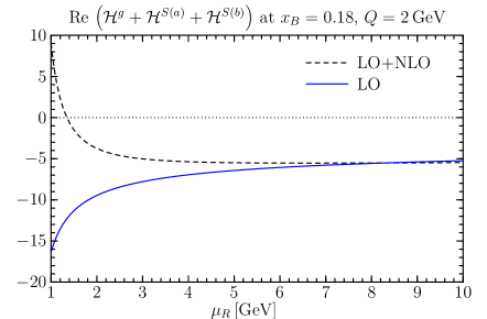
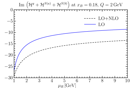
Refer to caption
Refer to caption
Refer to caption
Refer to caption
Refer to caption
Refer to caption
Figure 12: Dependence of the convolutions on μRsubscript𝜇𝑅\mu_{R}. The factorization scale is held fixed at μGPD=Qsubscript𝜇𝐺𝑃𝐷𝑄\mu_{GPD}=Q.
Refer to caption
Refer to caption
Refer to caption
Refer to caption
Refer to caption
Refer to caption
Figure 13: Dependence of the convolutions on μGPDsubscript𝜇𝐺𝑃𝐷\mu_{GPD}. The renormalization scale is held fixed at μR=Qsubscript𝜇𝑅𝑄\mu_{R}=Q.
Refer to caption
Refer to caption
Refer to caption
Refer to caption
Refer to caption
Refer to caption
Figure 14: Dependence of the convolutions on the common scale μ=μR=μGPD=μDA𝜇subscript𝜇𝑅subscript𝜇𝐺𝑃𝐷subscript𝜇𝐷𝐴\mu=\mu_{R}=\mu_{GPD}=\mu_{DA}.

Figure 12 shows the dependence of the convolutions on μRsubscript𝜇𝑅\mu_{R} at fixed μGPD=Qsubscript𝜇𝐺𝑃𝐷𝑄\mu_{GPD}=Q. Within the μRsubscript𝜇𝑅\mu_{R} range shown we generally find a moderate scale dependence, both at LO and at NLO. An exception is the region μR<2GeVsuperscriptsimilar-tosubscript𝜇𝑅2GeV\mu_{R}\raisebox{-4.0pt}{$\,\stackrel{{\scriptstyle\textstyle<}}{{\sim}}\,$}2\operatorname{GeV}, where the growth of the LO results simply reflects the growth of αs(μR)subscript𝛼𝑠subscript𝜇𝑅\alpha_{s}(\mu_{R}). Note that with the parameters specified at beginning of Sect. 4 we have αs(3)(2GeV)=0.30superscriptsubscript𝛼𝑠32GeV0.30\alpha_{\smash{s}}^{(3)}(2\operatorname{GeV})=0.30 and αs(3)(1GeV)=0.51superscriptsubscript𝛼𝑠31GeV0.51\alpha_{\smash{s}}^{(3)}(1\operatorname{GeV})=0.51. The NLO results further contain explicit logarithms ln(Q2/μR2)superscript𝑄2superscriptsubscript𝜇𝑅2\ln(Q^{2}/\mu_{R}^{2}), which in some cases can cause corrections to grow out of control, especially for the real parts of convolutions. We note that for Re(8)Resuperscript8\operatorname{Re}\mathcal{H}^{(8)} the NLO correction is is unusually large compared with the LO term. This is because of a nearby zero in xBsubscript𝑥𝐵x_{B}, as is seen in Fig. 9, and should not be a reason of particular concern.

The variation of the convolutions with μGPDsubscript𝜇𝐺𝑃𝐷\mu_{GPD} at fixed μR=Qsubscript𝜇𝑅𝑄\mu_{R}=Q is shown in Fig. 13. We again find a rather moderate scale dependence, except when μGPDsubscript𝜇𝐺𝑃𝐷\mu_{GPD} becomes small. The dependence on a single scale μ=μR=μGPD𝜇subscript𝜇𝑅subscript𝜇𝐺𝑃𝐷\mu=\mu_{R}=\mu_{GPD} is shown in Fig. 14. Note that in many cases the individual variation of μRsubscript𝜇𝑅\mu_{R} decreases the amplitude in absolute size whereas the variation of μGPDsubscript𝜇𝐺𝑃𝐷\mu_{GPD} increases it, with both tendencies partially canceling when the scales are set equal. Again we find that the scale dependence becomes quite drastic below 2GeV2GeV2\operatorname{GeV}.

We finally discuss the dependence on μDAsubscript𝜇𝐷𝐴\mu_{DA} for Gegenbauer indices n>0𝑛0n>0. According to (18) the convolutions n(μDA)subscript𝑛subscript𝜇𝐷𝐴\mathcal{H}_{n}(\mu_{DA}) appear multiplied by an(μDA)subscript𝑎𝑛subscript𝜇𝐷𝐴a_{n}(\mu_{DA}) in the process amplitude, where the scale dependence of both factors partially cancels. In Fig. 15 we therefore plot convolutions multiplied with a2(μDA)/a2(μ0)=[αs(μDA)/αs(μ0)]γ2/β0a_{2}(\mu_{DA})/a_{2}(\mu_{0})=\bigl{[}\alpha_{s}(\mu_{DA})/\alpha_{s}(\mu_{0})\bigr{]}{}^{\gamma_{2}/\beta_{0}} following the relation (16). The corresponding plots for n=4𝑛4n=4 and for convolutions in the quark non-singlet sector look very similar. We find that the dependence on μDAsubscript𝜇𝐷𝐴\mu_{DA} is slightly decreased when going to NLO.
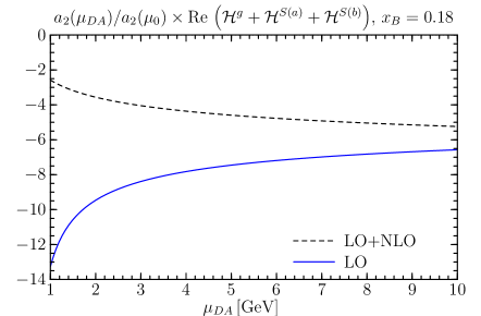
Refer to caption
Refer to caption
Figure 15: Dependence on the factorization scale μDAsubscript𝜇𝐷𝐴\mu_{DA} of the convolutions in the gluon and quark singlet sector multiplied by the scale dependence a2(μDA)/a2(μ0)subscript𝑎2subscript𝜇𝐷𝐴subscript𝑎2subscript𝜇0a_{2}(\mu_{DA})/a_{2}(\mu_{0}) of the corresponding Gegenbauer coefficient. The reference scale for a2subscript𝑎2a_{2} is taken as μ0=2GeVsubscript𝜇02GeV\mu_{0}=2\operatorname{GeV}, and the other scales are set to μGPD=μR=Q=2GeVsubscript𝜇𝐺𝑃𝐷subscript𝜇𝑅𝑄2GeV\mu_{GPD}=\mu_{R}=Q=2\operatorname{GeV}.

6 Proton helicity flip amplitudes

We now turn to the convolutions of the hard-scattering kernels with the GPDs describing proton helicity flip. In this section we take t=0.4GeV2𝑡0.4superscriptGeV2t=-0.4\operatorname{GeV}^{2}, which is the value for which will present estimates for observables in the next section.
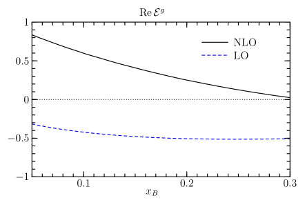
Refer to caption
Refer to caption
Refer to caption
Refer to caption
Refer to caption
Refer to caption
Figure 16: LO and NLO terms of the convolutions in the gluon and quark singlet sector for model 1 at Q=2GeV𝑄2GeVQ=2\operatorname{GeV} and t=0.4GeV2𝑡0.4superscriptGeV2t=-0.4\operatorname{GeV}^{2}. The scales are set to μR=μGPD=Qsubscript𝜇𝑅subscript𝜇𝐺𝑃𝐷𝑄\mu_{R}=\mu_{GPD}=Q.
Refer to caption
Refer to caption
Refer to caption
Refer to caption
Refer to caption
Refer to caption
Figure 17: As Fig. 16 but for model 2.
Refer to caption
Refer to caption
Refer to caption
Refer to caption
Figure 18: LO and NLO terms of the convolutions in the quark non-singlet sector for model 1 at Q=2GeV𝑄2GeVQ=2\operatorname{GeV} and t=0.4GeV2𝑡0.4superscriptGeV2t=-0.4\operatorname{GeV}^{2}, with μR=μGPD=Qsubscript𝜇𝑅subscript𝜇𝐺𝑃𝐷𝑄\mu_{R}=\mu_{GPD}=Q.
Refer to caption
Refer to caption
Refer to caption
Refer to caption
Figure 19: As Fig. 18 but for model 2.

In Figs. 16 and 17 we compare the LO and NLO terms of the convolutions in the gluon and quark singlet sector for the two models described in Sect. 3.1. For model 1 the individual corrections for gluon and quark convolutions look quite similar to those we saw for \mathcal{H} in the previous section. The sum of gluon and quark singlet contributions at LO is however very small in this model because of cancellations, so that the NLO term dominates in a wide kinematical region. In model 2 the gluon contributions are nearly absent, so that the quark singlet contribution dominates in this sector. We note that, contrary to the individual terms, the sum of gluon and quark singlet contributions comes out to be rather similar in the two models and is small compared with the flavor non-singlet contributions shown in Figs. 18 and 19. According to our discussion at the end of Sect. 3.1 this has its origin in the sum rule (3.1) for the second moment of E𝐸E at t=0𝑡0t=0, so that we expect a small net contribution from gluons and the quark singlet in large class of models for E𝐸E.

As shown in Figs. 18 and 19, the NLO corrections to the quark non-singlet convolutions are relatively moderate but not small, similarly to the case of \mathcal{H}. The size of the convolutions is quite different in the two models, indicating the important role played at intermediate xBsubscript𝑥𝐵x_{B} by sea quarks in model 1. Let us recall that with the double distribution ansatz (3.1) the GPDs at xξsimilar-to𝑥𝜉x\sim\xi are sensitive to forward parton distributions with momentum fractions well below ξ𝜉\xi, as discussed in Sect. 4.3.3 of [17].

7 Cross sections and asymmetries

Having studied in detail the building blocks of the scattering amplitude for vector meson production, we now combine them to observables. We recall that to leading order in 1/Q1𝑄1/Q there are just two of these: the unpolarized γpsuperscript𝛾𝑝\gamma^{*}p cross section and the asymmetry for a transversely polarized target, both referring to longitudinal polarization of virtual photon and produced meson. The ep𝑒𝑝ep cross section in the leading 1/Q1𝑄1/Q approximation can be written as

dσ(epepV)dtdQ2dydϕdϕS=α4π31xBQ21yydσLdt[1+STsin(ϕϕS)AUT]𝑑𝜎𝑒𝑝𝑒𝑝𝑉𝑑𝑡𝑑superscript𝑄2𝑑𝑦𝑑italic-ϕ𝑑subscriptitalic-ϕ𝑆𝛼4superscript𝜋31subscript𝑥𝐵superscript𝑄21𝑦𝑦𝑑subscript𝜎𝐿𝑑𝑡delimited-[]1subscript𝑆𝑇italic-ϕsubscriptitalic-ϕ𝑆subscript𝐴𝑈𝑇\frac{d\sigma(ep\to epV)}{dt\,dQ^{2}\,dy\,d\phi\,d\phi_{S}}=\frac{\alpha}{4\pi^{3}}\,\frac{1-x_{B}}{Q^{2}}\,\frac{1-y}{y}\,\frac{d\sigma_{L}}{dt}\Bigl{[}1+S_{T}\sin(\phi-\phi_{S})\mskip 1.5muA_{UT}\Bigr{]} (60)

where y𝑦y is the usual inelasticity variable for deep inelastic scattering and STsubscript𝑆𝑇S_{T} denotes the transverse component of the target polarization. ϕitalic-ϕ\phi is the azimuthal angle between lepton plane and hadron plane, and ϕSsubscriptitalic-ϕ𝑆\phi_{S} is the azimuthal angle between lepton plane and target spin vector, both defined according to the Trento convention [40]. The γpsuperscript𝛾𝑝\gamma^{*}p cross section dσL/dt𝑑subscript𝜎𝐿𝑑𝑡d\sigma_{L}/dt and the polarization asymmetry AUTsubscript𝐴𝑈𝑇A_{UT} depend on xBsubscript𝑥𝐵x_{B}, Q2superscript𝑄2Q^{2} and t𝑡t. To leading order in 1/Q1𝑄1/Q they are given by

dσLdt𝑑subscript𝜎𝐿𝑑𝑡\displaystyle\frac{d\sigma_{L}}{dt} =π29αQ6(2xB)21xBfV2[(1ξ2)|V|2(t/(4mp2)+ξ2)|V|22ξ2Re(VV)]absentsuperscript𝜋29𝛼superscript𝑄6superscript2subscript𝑥𝐵21subscript𝑥𝐵superscriptsubscript𝑓𝑉2delimited-[]1superscript𝜉2superscriptsubscript𝑉2𝑡4superscriptsubscript𝑚𝑝2superscript𝜉2superscriptsubscript𝑉22superscript𝜉2Resuperscriptsubscript𝑉subscript𝑉\displaystyle=\frac{\pi^{2}}{9}\,\frac{\alpha}{Q^{6}}\,\frac{(2-x_{B})^{2}}{1-x_{B}}\,f_{V}^{2}\,\Bigl{[}\mskip 1.5mu(1-\xi^{2})\,|\mathcal{H}_{V}|^{2}-\bigl{(}\mskip 1.5mut/(4m_{p}^{2})+\xi^{2}\mskip 1.5mu\bigr{)}\,|\mathcal{E}_{V}|^{2}-2\xi^{2}\operatorname{Re}\bigl{(}\mathcal{E}_{V}^{*}\mskip 1.5mu\mathcal{H}_{V}\bigr{)}\mskip 1.5mu\Bigr{]} (61)
and
AUTsubscript𝐴𝑈𝑇\displaystyle A_{UT} =t0tmp1ξ2Im(VV)(1ξ2)|V|2(t/(4mp2)+ξ2)|V|22ξ2Re(VV),absentsubscript𝑡0𝑡subscript𝑚𝑝1superscript𝜉2Imsuperscriptsubscript𝑉subscript𝑉1superscript𝜉2superscriptsubscript𝑉2𝑡4superscriptsubscript𝑚𝑝2superscript𝜉2superscriptsubscript𝑉22superscript𝜉2Resuperscriptsubscript𝑉subscript𝑉\displaystyle=\frac{\sqrt{t_{0}-t\rule{0.0pt}{7.74998pt}}}{m_{p}}\,\frac{\sqrt{1-\xi^{2}}\,\operatorname{Im}\bigl{(}\mathcal{E}_{V}^{*}\mskip 1.5mu\mathcal{H}_{V}\bigr{)}}{\rule{0.0pt}{10.00002pt}(1-\xi^{2})\,|\mathcal{H}_{V}|^{2}-\bigl{(}\mskip 1.5mut/(4m_{p}^{2})+\xi^{2}\mskip 1.5mu\bigr{)}\,|\mathcal{E}_{V}|^{2}-2\xi^{2}\operatorname{Re}\bigl{(}\mathcal{E}_{V}^{*}\mskip 1.5mu\mathcal{H}_{V}\bigr{)}}\,, (62)

where t0=4mp2ξ2/(1ξ2)subscript𝑡04superscriptsubscript𝑚𝑝2superscript𝜉21superscript𝜉2t_{0}=-4m_{p}^{2}\mskip 1.5mu\xi^{2}/(1-\xi^{2}). Here we have combined the convolutions (2.1) into

V=QVn=0an[ng+nS(a)+nS(b)+eV(3)n(3)+eV(8)n(8)],subscript𝑉subscript𝑄𝑉superscriptsubscript𝑛0subscript𝑎𝑛delimited-[]subscriptsuperscript𝑔𝑛subscriptsuperscript𝑆𝑎𝑛subscriptsuperscript𝑆𝑏𝑛superscriptsubscript𝑒𝑉3subscriptsuperscript3𝑛superscriptsubscript𝑒𝑉8subscriptsuperscript8𝑛\mathcal{F}_{V}=Q_{V}\sum_{n=0}^{\infty}a_{n}\mskip 1.5mu\biggl{[}\mathcal{F}^{g}_{n}+\mathcal{H}^{S(a)}_{n}+\mathcal{F}^{S(b)}_{n}+e_{V}^{(3)}\,\mathcal{F}^{(3)}_{n\phantom{V}}+e_{V}^{(8)}\,\mathcal{F}^{(8)}_{n\phantom{V}}\biggr{]}\,, (63)

with analogous combinations for Vsubscript𝑉\mathcal{H}_{V} and Vsubscript𝑉\mathcal{E}_{V}. In the remainder of this section we take the asymptotic form of the meson distribution amplitude, i.e. we set an=0subscript𝑎𝑛0a_{n}=0 for n2𝑛2n\geq 2. As long as Vsubscript𝑉\mathcal{E}_{V} is not much larger than Vsubscript𝑉\mathcal{H}_{V}, the cross section (61) is dominated by the term with |V|2superscriptsubscript𝑉2|\mathcal{H}_{V}|^{2} in a wide range of kinematics, where the prefactors ξ2superscript𝜉2\xi^{2} and t/(4mp2)𝑡4superscriptsubscript𝑚𝑝2t/(4m_{p}^{2}) of the other terms are small. The asymmetry (62) is then approximately given by

AUTt0tmpIm(VV)|V|2=t0tmp|VV|sinδV,A_{UT}\approx\frac{\sqrt{t_{0}-t\rule{0.0pt}{7.74998pt}}}{m_{p}}\;\frac{\operatorname{Im}\bigl{(}\mathcal{E}_{V}^{*}\mskip 1.5mu\mathcal{H}_{V}\bigr{)}}{|\mathcal{H}_{V}|^{2}}=\frac{\sqrt{t_{0}-t\rule{0.0pt}{7.74998pt}}}{m_{p}}\;\biggl{|}\frac{\mathcal{E}_{V}}{\mathcal{H}_{V}}\,\biggr{|}\sin\delta_{V}\,, (64)

where δV=arg(V/V)subscript𝛿𝑉subscript𝑉subscript𝑉\delta_{V}=\arg(\mathcal{H}_{V}/\mathcal{E}_{V}) is the relative phase between Vsubscript𝑉\mathcal{H}_{V} and Vsubscript𝑉\mathcal{E}_{V}.

Figure 21 shows the real and imaginary parts of the convolutions appearing in (61) and (62). ρsubscript𝜌\mathcal{H}_{\rho} is dominated by the gluon and quark singlet part, and in line with our discussion in Sect. 5 we find rather moderate corrections for the imaginary part but a very unstable real part in a wide range of xBsubscript𝑥𝐵x_{B}. As for ρsubscript𝜌\mathcal{E}_{\rho}, its real part is very small and subject to large relative corrections, whereas its imaginary part is much larger and receives corrections of order 100%percent100100\% . As we see in Fig. 18, the individual flavor non-singlet combinations (3)superscript3\mathcal{E}^{(3)} and (8)superscript8\mathcal{E}^{(8)} are less affected by corrections, but they have opposite sign and partially cancel in the sum relevant for ρ𝜌\rho production. The rather small but unstable contribution from the gluon and quark singlet terms is hence important in this channel and largely responsible for the NLO corrections seen in Fig. 21. As a further consequence of the cancellations just mentioned, the size of ρsubscript𝜌\mathcal{E}_{\rho} is tiny compared with ρsubscript𝜌\mathcal{H}_{\rho}. The quark flavor combination relevant for ρ𝜌\rho production is 2u+d2𝑢𝑑2u+d, where in our model the flavor combinations add for H𝐻H but largely cancel for E𝐸E.

Refer to caption
Refer to caption
Figure 20: Real and imaginary parts of the convolutions (63) for ρ𝜌\rho production at Q=2GeV𝑄2GeVQ=2\operatorname{GeV} and t=0.4GeV2𝑡0.4superscriptGeV2t=-0.4\operatorname{GeV}^{2}, with model 1 taken for the proton helicity-flip distributions. The scales are set to μR=μGPD=Qsubscript𝜇𝑅subscript𝜇𝐺𝑃𝐷𝑄\mu_{R}=\mu_{GPD}=Q.
Refer to caption
Refer to caption
Figure 21: As Fig. 21 but for ω𝜔\omega production.

For ω𝜔\omega production we see in Fig. 21 that at smaller xBsubscript𝑥𝐵x_{B} the convolution ωsubscript𝜔\mathcal{H}_{\omega} is about 1/3131/3 of ρsubscript𝜌\mathcal{H}_{\rho}, which follows from the dominance of the gluon contribution as seen in (6) and (7), whereas at larger xBsubscript𝑥𝐵x_{B} differences between the two channels appear. ωsubscript𝜔\mathcal{E}_{\omega} is much bigger than ρsubscript𝜌\mathcal{E}_{\rho} since in the combination 2ud2𝑢𝑑2u-d the contributions of u𝑢u and d𝑑d quarks add for E𝐸E, and the size of its radiative corrections reflects the one of (3)superscript3\mathcal{E}^{(3)} in Fig. 18. We note that the dominance of the imaginary over the real part in ωsubscript𝜔\mathcal{E}_{\omega} and ρsubscript𝜌\mathcal{E}_{\rho} is less pronounced in model 2, as can be anticipated by comparing Figs. 18 and 19.

The cross section dσL/dt𝑑subscript𝜎𝐿𝑑𝑡d\sigma_{L}/dt for ρ𝜌\rho production is dominated by (Imρ)2superscriptImsubscript𝜌2(\operatorname{Im}\mathcal{H}_{\rho})^{2}, except for contributions from (Reρ)2superscriptResubscript𝜌2(\operatorname{Re}\mathcal{H}_{\rho})^{2} at small xBsubscript𝑥𝐵x_{B} for NLO and at large xBsubscript𝑥𝐵x_{B} for LO. Given the size of corrections to ImρImsubscript𝜌\operatorname{Im}\mathcal{H}_{\rho} in Fig. 21 we thus have quite substantial NLO effects in the cross section at Q2=4GeV2superscript𝑄24superscriptGeV2Q^{2}=4\operatorname{GeV}^{2}, as shown in Fig. 24. For Q2=9GeV2superscript𝑄29superscriptGeV2Q^{2}=9\operatorname{GeV}^{2} and xB>0.1subscript𝑥𝐵0.1x_{B}>0.1 the relative corrections decrease. The plot has been calculated with model 1 for E𝐸E, but since its contribution to dσL/dt𝑑subscript𝜎𝐿𝑑𝑡d\sigma_{L}/dt is negligible the corresponding curves for model 2 look very similar. To obtain an estimate of scale uncertainties, we show bands corresponding to μ=μR=μGPD𝜇subscript𝜇𝑅subscript𝜇𝐺𝑃𝐷\mu=\mu_{R}=\mu_{GPD} between 2GeV2GeV2\operatorname{GeV} and 2Q2𝑄2Q. Given our discussion in the previous section, we do not consider it meaningful to go to scales below 2GeV2GeV2\operatorname{GeV}, so that the bands in the figure are strongly asymmetric. For Q2=4GeV2superscript𝑄24superscriptGeV2Q^{2}=4\operatorname{GeV}^{2} they go only in one direction, and the band of the LO result does not provide an estimate for the size of the NLO corrections, which turn out to go in the other direction.

We have a very peculiar situation for the polarization asymmetry AUTsubscript𝐴𝑈𝑇A_{UT} in ρ𝜌\rho production, which as shown in Figs. 24 and 24 is very small in both models 1 and 2 due to the cancellations in ρsubscript𝜌\mathcal{E}_{\rho} discussed above. AUTsubscript𝐴𝑈𝑇A_{UT} changes quite dramatically from LO to NLO in a wide range of kinematics, clearly because of the NLO corrections in the numerator. A closer look at Fig. 21 reveals that the large perturbative corrections in Im(ρρ)Imsuperscriptsubscript𝜌subscript𝜌\operatorname{Im}\bigl{(}\mathcal{E}_{\rho}^{*}\mskip 1.5mu\mathcal{H}_{\rho}\bigr{)} are mainly due to the large corrections to both ReρResubscript𝜌\operatorname{Re}\mathcal{H}_{\rho} and ReρResubscript𝜌\operatorname{Re}\mathcal{E}_{\rho}. These hardly affect the unpolarized cross section, which is strongly dominated by ImρImsubscript𝜌\operatorname{Im}\mathcal{H}_{\rho}. At higher Q2superscript𝑄2Q^{2} the instability of AUTsubscript𝐴𝑈𝑇A_{UT} is less pronounced, and in model 2 we even have quite small corrections. We note that the bands from the scale variation at LO order are extremely narrow in Figs. 24 and 24. This is because the scale variation of αs(μR)subscript𝛼𝑠subscript𝜇𝑅\alpha_{s}(\mu_{R}) cancels in the ratio AUTsubscript𝐴𝑈𝑇A_{UT} at LO and because in the kinematics we are looking at, the μGPDsubscript𝜇𝐺𝑃𝐷\mu_{GPD} dependence of ρsubscript𝜌\mathcal{H}_{\rho} and ρsubscript𝜌\mathcal{E}_{\rho} is rather weak. In this situation, the scale uncertainty of the LO result does obviously not provide a good estimate for the size of higher-order corrections. Let us finally remark that at t=0.4GeV2𝑡0.4superscriptGeV2t=-0.4\operatorname{GeV}^{2} the asymmetry AUTsubscript𝐴𝑈𝑇A_{UT} must go to zero as xBsubscript𝑥𝐵x_{B} tends to 0.4840.4840.484 because of the prefactor t0tsubscript𝑡0𝑡\sqrt{t_{0}-t\rule{0.0pt}{7.74998pt}} in (62).

The cross section for ω𝜔\omega production is shown in Fig. 27 and shows a similar pattern of NLO corrections to the one in ρ𝜌\rho production, reflecting the similar pattern of corrections we have seen for ImρImsubscript𝜌\operatorname{Im}\mathcal{H}_{\rho} and ImωImsubscript𝜔\operatorname{Im}\mathcal{H}_{\omega}. As a result the ratio of cross sections dσL/dt𝑑subscript𝜎𝐿𝑑𝑡d\sigma_{L}/dt in the two channels is quite stable under radiative corrections, as seen in Fig. 27. The target polarization asymmetry, shown in Fig. 27 for model 1, changes however drastically between LO and NLO at small to intermediate xBsubscript𝑥𝐵x_{B}. This is because ImωImsubscript𝜔\operatorname{Im}\mathcal{E}_{\omega} then dominates over ReωResubscript𝜔\operatorname{Re}\mathcal{E}_{\omega}, so that its product with the unstable convolution ReωResubscript𝜔\operatorname{Re}\mathcal{H}_{\omega} controls the numerator of the asymmetry. The absolute size of AUTsubscript𝐴𝑈𝑇A_{UT} can be large in this channel since |ω||ω|similar-tosubscript𝜔subscript𝜔|\mathcal{E}_{\omega}|\sim|\mathcal{H}_{\omega}| in our model. According to Fig. 21, the relative phase δωsubscript𝛿𝜔\delta_{\omega} is close to zero at LO for xB<0.3superscriptsimilar-tosubscript𝑥𝐵0.3x_{B}\raisebox{-4.0pt}{$\,\stackrel{{\scriptstyle\textstyle<}}{{\sim}}\,$}0.3, so that the factor sinδωsubscript𝛿𝜔\sin\delta_{\omega} in (64) makes AUTsubscript𝐴𝑈𝑇A_{UT} small and prone to large radiative corrections.

Let us finally take a look at ϕitalic-ϕ\phi production. At LO this channel is strongly dominated by gluon exchange, since in our models strange quark distributions are small for H𝐻H and even more so for E𝐸E. At NLO we have further contributions from the pure singlet terms S(b)superscript𝑆𝑏\mathcal{H}^{S(b)} and S(b)superscript𝑆𝑏\mathcal{E}^{S(b)}, which are not negligible. We see in Fig. 30 that the NLO corrections to the cross section are large at small xBsubscript𝑥𝐵x_{B} and slowly decrease with xBsubscript𝑥𝐵x_{B}. Except for the region of small xBsubscript𝑥𝐵x_{B}, this pattern is quite different from the one in ρ𝜌\rho production, so that the cross section ratio for the two channels receives important corrections at larger xBsubscript𝑥𝐵x_{B} as we see in Fig. 30. The asymmetry AUTsubscript𝐴𝑈𝑇A_{UT} is essentially zero at LO, because in our model the relative phase δϕsubscript𝛿italic-ϕ\delta_{\phi} between ϕsubscriptitalic-ϕ\mathcal{H}_{\phi} and ϕsubscriptitalic-ϕ\mathcal{E}_{\phi} is very close to zero. This changes at NLO, where in model 1 we obtain a small to moderate AUTsubscript𝐴𝑈𝑇A_{UT}, as shown in Fig. 30.
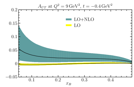
Refer to caption
Refer to caption
Figure 22: Longitudinal cross section for γpρpsuperscript𝛾𝑝𝜌𝑝\gamma^{*}p\to\rho\mskip 1.5mup in model 1. Bands correspond to the range 2GeV<μ<4GeV2GeV𝜇4GeV2\operatorname{GeV}<\mu<4\operatorname{GeV} in the left and to 2GeV<μ<6GeV2GeV𝜇6GeV2\operatorname{GeV}<\mu<6\operatorname{GeV} in the right plot, and solid lines to μ=Q𝜇𝑄\mu=Q in both cases.
Refer to caption
Refer to caption
Figure 23: The transverse target spin asymmetry defined in (60), calculated for model 1. The meaning of the bands and solid lines is as in Fig. 24.
Refer to caption
Refer to caption
Figure 24: As Fig. 24 but for model 2.
Refer to caption
Refer to caption
Figure 25: As Fig. 24 but for γpωpsuperscript𝛾𝑝𝜔𝑝\gamma^{*}p\to\omega\mskip 1.5mup.
Refer to caption
Refer to caption
Figure 26: Ratio of cross sections dσL/dt𝑑subscript𝜎𝐿𝑑𝑡d\sigma_{L}/dt for ω𝜔\omega and ρ𝜌\rho production in model 1. The meaning of the bands and solid lines is as in Fig. 24.
Refer to caption
Refer to caption
Figure 27: As Fig. 24 but for γpωpsuperscript𝛾𝑝𝜔𝑝\gamma^{*}p\to\omega\mskip 1.5mup.
Refer to caption
Refer to caption
Figure 28: As Fig. 24 but for γpϕpsuperscript𝛾𝑝italic-ϕ𝑝\gamma^{*}p\to\phi\mskip 1.5mup.
Refer to caption
Refer to caption
Figure 29: Ratio of cross sections dσL/dt𝑑subscript𝜎𝐿𝑑𝑡d\sigma_{L}/dt for ϕitalic-ϕ\phi and ρ𝜌\rho production in model 1. The meaning of the bands and solid lines is as in Fig. 24.
Refer to caption
Refer to caption
Figure 30: As Fig. 24 but for γpϕpsuperscript𝛾𝑝italic-ϕ𝑝\gamma^{*}p\to\phi\mskip 1.5mup.

8 Pseudoscalar meson production

Having studied in detail the production of vector mesons, let us finally take a look at pseudoscalar production. We will only consider γpπ+nsuperscript𝛾𝑝superscript𝜋𝑛\gamma^{*}p\to\pi^{+}n, which was already studied at NLO in [10]. Gluon distributions do not contribute in this channel.

In the collinear approximation the amplitude for this process can be written as

\displaystyle\mathcal{M} =4π4παξQNcfπ01𝑑zϕπ(z)11𝑑x[euTa(z¯,x,ξ)edTa(z,x,ξ)][F~u(x,ξ,t)F~d(x,ξ,t)]absent4𝜋4𝜋𝛼𝜉𝑄subscript𝑁𝑐subscript𝑓𝜋superscriptsubscript01differential-d𝑧subscriptitalic-ϕ𝜋𝑧superscriptsubscript11differential-d𝑥delimited-[]subscript𝑒𝑢subscript𝑇𝑎¯𝑧𝑥𝜉subscript𝑒𝑑subscript𝑇𝑎𝑧𝑥𝜉delimited-[]superscript~𝐹𝑢𝑥𝜉𝑡superscript~𝐹𝑑𝑥𝜉𝑡\displaystyle=\frac{4\pi\sqrt{4\pi\alpha}}{\xi\mskip 1.5muQN_{c}}\,f_{\pi}\int_{0}^{1}dz\,\phi_{\pi}(z)\int_{-1}^{1}dx\,\Bigl{[}e_{u}\mskip 1.5muT_{a}(\bar{z},x,\xi)-e_{d}\mskip 1.5muT_{a}(z,-x,\xi)\Bigr{]}\,\Bigl{[}\widetilde{F}^{u}(x,\xi,t)-\widetilde{F}^{d}(x,\xi,t)\Bigr{]}
=4π4παξQNcfπn=0an~nπabsent4𝜋4𝜋𝛼𝜉𝑄subscript𝑁𝑐subscript𝑓𝜋superscriptsubscript𝑛0subscript𝑎𝑛subscriptsuperscript~𝜋𝑛\displaystyle=\frac{4\pi\sqrt{4\pi\alpha}}{\xi\mskip 1.5muQN_{c}}\,f_{\pi}\sum_{n=0}^{\infty}a_{n}\mskip 1.5mu\widetilde{\mathcal{F}}^{\mskip 1.5mu\pi}_{n} (65)

with eu=2/3subscript𝑒𝑢23e_{u}=2/3, ed=1/3subscript𝑒𝑑13e_{d}=-1/3 and fπ=131MeVsubscript𝑓𝜋131MeVf_{\pi}=131\operatorname{MeV}. ϕπ(z)subscriptitalic-ϕ𝜋𝑧\phi_{\pi}(z) is the twist-two distribution amplitude of the pion and has a Gegenbauer decomposition as in (15). The convolutions ~nπsubscriptsuperscript~𝜋𝑛\widetilde{\mathcal{F}}^{\mskip 1.5mu\pi}_{n} are defined as

~nπ=11𝑑x[euTa,n(x,ξ)edTa(x,ξ)][F~u(x,ξ,t)F~d(x,ξ,t)],subscriptsuperscript~𝜋𝑛superscriptsubscript11differential-d𝑥delimited-[]subscript𝑒𝑢subscript𝑇𝑎𝑛𝑥𝜉subscript𝑒𝑑subscript𝑇𝑎𝑥𝜉delimited-[]superscript~𝐹𝑢𝑥𝜉𝑡superscript~𝐹𝑑𝑥𝜉𝑡\widetilde{\mathcal{F}}^{\mskip 1.5mu\pi}_{n}=\int_{-1}^{1}dx\,\Bigl{[}e_{u}\mskip 1.5muT_{a,n}(x,\xi)-e_{d}\mskip 1.5muT_{a}(-x,\xi)\Bigr{]}\,\Bigl{[}\widetilde{F}^{u}(x,\xi,t)-\widetilde{F}^{d}(x,\xi,t)\Bigr{]}\,, (66)

and the kernels Ta(z¯,x,ξ)subscript𝑇𝑎¯𝑧𝑥𝜉T_{a}(\bar{z},x,\xi) and Ta,n(x,ξ)subscript𝑇𝑎𝑛𝑥𝜉T_{a,n}(x,\xi) are the same as in Sect. 2. The matrix elements F~qsuperscript~𝐹𝑞\widetilde{F}^{q} are the counterparts of Fqsuperscript𝐹𝑞F^{q} for polarized quarks and given by

F~q(x,ξ,t)=1(p+p)n[H~q(x,ξ,t)u¯(p)γ5u(p)+E~q(x,ξ,t)u¯(p)(pp)n2mpγ5u(p)]superscript~𝐹𝑞𝑥𝜉𝑡1𝑝superscript𝑝𝑛delimited-[]superscript~𝐻𝑞𝑥𝜉𝑡¯𝑢superscript𝑝italic-n̸subscript𝛾5𝑢𝑝superscript~𝐸𝑞𝑥𝜉𝑡¯𝑢superscript𝑝superscript𝑝𝑝𝑛2subscript𝑚𝑝subscript𝛾5𝑢𝑝\widetilde{F}^{q}(x,\xi,t)=\frac{1}{(p+p^{\prime})\cdot n}\left[\widetilde{H}^{q}(x,\xi,t)\,\bar{u}(p^{\prime})\mskip 1.5mu\not{n}\gamma_{5}\mskip 1.5muu(p)+\widetilde{E}^{q}(x,\xi,t)\,\bar{u}(p^{\prime})\,\frac{(p^{\prime}-p)\cdot n}{2m_{p}}\,\gamma_{5}\mskip 1.5muu(p)\right] (67)

in terms of the generalized parton distributions H~~𝐻\widetilde{H} and E~~𝐸\widetilde{E}, where as in the unpolarized case we use the conventions of [17]. Since the hard-scattering kernel in (66) is neither even nor odd in x𝑥x, the convolution involves both the charge-conjugation even and odd combinations

F~q(+)(x,ξ,t)superscript~𝐹𝑞𝑥𝜉𝑡\displaystyle\widetilde{F}^{q(+)}(x,\xi,t) =F~q(x,ξ,t)+F~q(x,ξ,t),absentsuperscript~𝐹𝑞𝑥𝜉𝑡superscript~𝐹𝑞𝑥𝜉𝑡\displaystyle=\widetilde{F}^{q}(x,\xi,t)+\widetilde{F}^{q}(-x,\xi,t)\,, F~q()(x,ξ,t)superscript~𝐹𝑞𝑥𝜉𝑡\displaystyle\widetilde{F}^{q(-)}(x,\xi,t) =F~q(x,ξ,t)F~q(x,ξ,t).absentsuperscript~𝐹𝑞𝑥𝜉𝑡superscript~𝐹𝑞𝑥𝜉𝑡\displaystyle=\widetilde{F}^{q}(x,\xi,t)-\widetilde{F}^{q}(-x,\xi,t)\,. (68)

We model the distributions H~~𝐻\widetilde{H} in close analogy to the unpolarized case and set

H~q(+)(x,ξ,t)superscript~𝐻𝑞𝑥𝜉𝑡\displaystyle\widetilde{H}^{q(+)}(x,\xi,t) =11𝑑β1+|β|1|β|𝑑αδ(xβξα)h(2)(β,α)H~q(+)(β,0,t),absentsuperscriptsubscript11differential-d𝛽superscriptsubscript1𝛽1𝛽differential-d𝛼𝛿𝑥𝛽𝜉𝛼superscript2𝛽𝛼superscript~𝐻𝑞𝛽0𝑡\displaystyle=\int_{-1}^{1}d\beta\int_{-1+|\beta|}^{1-|\beta|}d\alpha\;\delta(x-\beta-\xi\alpha)\,h^{(2)}(\beta,\alpha)\,\widetilde{H}^{q(+)}(\beta,0,t)\,,
H~q()(x,ξ,t)superscript~𝐻𝑞𝑥𝜉𝑡\displaystyle\widetilde{H}^{q(-)}(x,\xi,t) =11𝑑β1+|β|1|β|𝑑αδ(xβξα)h(2)(β,α)H~q()(β,0,t),absentsuperscriptsubscript11differential-d𝛽superscriptsubscript1𝛽1𝛽differential-d𝛼𝛿𝑥𝛽𝜉𝛼superscript2𝛽𝛼superscript~𝐻𝑞𝛽0𝑡\displaystyle=\int_{-1}^{1}d\beta\int_{-1+|\beta|}^{1-|\beta|}d\alpha\;\delta(x-\beta-\xi\alpha)\,h^{(2)}(\beta,\alpha)\,\widetilde{H}^{q(-)}(\beta,0,t)\,, (69)

with h(2)(β,α)superscript2𝛽𝛼h^{(2)}(\beta,\alpha) as in (24) and

H~q(+)(x,0,t)superscript~𝐻𝑞𝑥0𝑡\displaystyle\widetilde{H}^{q(+)}(x,0,t) =Δqv(x)exp[tfqv(x)]+2Δq¯(x)exp[tfq¯(x)],absentΔsubscript𝑞𝑣𝑥𝑡subscript𝑓subscript𝑞𝑣𝑥2Δ¯𝑞𝑥𝑡subscript𝑓¯𝑞𝑥\displaystyle=\Delta q_{v}(x)\exp\bigl{[}tf_{q_{v}}(x)\bigr{]}+2\Delta\bar{q}(x)\exp\bigl{[}tf_{\bar{q}}(x)\bigr{]}\,,
H~q()(x,0,t)superscript~𝐻𝑞𝑥0𝑡\displaystyle\widetilde{H}^{q(-)}(x,0,t) =Δqv(x)exp[tfqv(x)]absentΔsubscript𝑞𝑣𝑥𝑡subscript𝑓subscript𝑞𝑣𝑥\displaystyle=\Delta q_{v}(x)\exp\bigl{[}tf_{q_{v}}(x)\bigr{]} (70)

for x>0𝑥0x>0. The values for x<0𝑥0x<0 are determined by the symmetry properties following from (68). For the polarized valence and antiquark densities ΔqvΔsubscript𝑞𝑣\Delta q_{v} and Δq¯Δ¯𝑞\Delta\bar{q} we use the NLO parameterization from [41] at μ=2GeV𝜇2GeV\mu=2\operatorname{GeV}, and for the t𝑡t dependence we take the same functions fqv(x)subscript𝑓subscript𝑞𝑣𝑥f_{q_{v}}(x) as in (26), (3) and furthermore set fq¯(x)=fqv(x)subscript𝑓¯𝑞𝑥subscript𝑓subscript𝑞𝑣𝑥f_{\bar{q}}(x)=f_{q_{v}}(x). As was shown in [28], this gives a good description of the isovector axial form factor via the sum rule

FA(t)=01dx[H~u(+)(x,0,t)H~d(+)(x,0,t)].F_{A}(t)=\int_{0}^{1}dx\,\bigl{[}\widetilde{H}^{u(+)}(x,0,t)-\widetilde{H}^{d(+)}(x,0,t)\bigl{]}\,. (71)

For the nucleon helicity-flip distribution E~~𝐸\widetilde{E} we take a pion exchange ansatz

E~u(x,ξ,t)=E~d(x,ξ,t)=θ(ξ|x|)2ξϕπ(x+ξ2ξ)2mp2gAmπ2tΛ2mπ2Λ2t,superscript~𝐸𝑢𝑥𝜉𝑡superscript~𝐸𝑑𝑥𝜉𝑡𝜃𝜉𝑥2𝜉subscriptitalic-ϕ𝜋𝑥𝜉2𝜉2superscriptsubscript𝑚𝑝2subscript𝑔𝐴superscriptsubscript𝑚𝜋2𝑡superscriptΛ2superscriptsubscript𝑚𝜋2superscriptΛ2𝑡\widetilde{E}^{u}(x,\xi,t)=-\widetilde{E}^{d}(x,\xi,t)=\frac{\theta\bigl{(}\xi-|x|\bigr{)}}{2\xi}\,\phi_{\pi}\left(\frac{x+\xi}{2\xi}\right)\frac{2m_{p}^{2}\,g_{A}}{m_{\pi}^{2}-t}\,\frac{\Lambda^{2}-m_{\pi}^{2}}{\Lambda^{2}-t}, (72)

with the nucleon axial charge gA1.26subscript𝑔𝐴1.26g_{A}\approx 1.26 and a cutoff parameter Λ=0.8GeVΛ0.8GeV\Lambda=0.8\operatorname{GeV} [42] to suppress large off-shellness of the exchanged pion in the t𝑡t channel.

8.1 Results

Refer to caption
Refer to caption
Figure 31: The convolution ~0πsubscriptsuperscript~𝜋0\widetilde{\mathcal{H}}^{\mskip 1.5mu\pi}_{\mskip 1.5mu0} defined as in (66), evaluated at Q=2GeV𝑄2GeVQ=2\operatorname{GeV} and t=0.4GeV2𝑡0.4superscriptGeV2t=-0.4\operatorname{GeV}^{2}. The scales are set to μR=μGPD=Qsubscript𝜇𝑅subscript𝜇𝐺𝑃𝐷𝑄\mu_{R}=\mu_{GPD}=Q.

The convolution ~nπsubscriptsuperscript~𝜋𝑛\widetilde{\mathcal{H}}^{\mskip 1.5mu\pi}_{n} at LO and NLO is shown in Fig. 31 for n=0𝑛0n=0. We find moderate corrections for the imaginary part and larger ones for the real part. For ~nπsubscriptsuperscript~𝜋𝑛\widetilde{\mathcal{E}}^{\mskip 1.5mu\pi}_{n} we can easily give the analytic form of the NLO result. The scale dependent terms admit a closed expression,

nan~nπm,namproportional-tosubscript𝑛subscript𝑎𝑛subscriptsuperscript~𝜋𝑛subscript𝑚𝑛subscript𝑎𝑚\displaystyle\sum_{n}a_{n}\mskip 1.5mu\widetilde{\mathcal{E}}^{\mskip 1.5mu\pi}_{n}\,\propto\,\sum_{m,n}a_{m} an{1+αs4π\displaystyle a_{n}\mskip 1.5mu\biggl{\{}1+\frac{\alpha_{s}}{4\pi}
×[β0(143+γm+γn2CFlnQ2μR2)γmlnQ2μGPD2γnlnQ2μDA2+]},\displaystyle\;\times\biggl{[}\,\beta_{0}\mskip 1.5mu\biggl{(}\frac{14}{3}+\frac{\gamma_{m}+\gamma_{n}}{2C_{F}}-\ln\frac{Q^{2}}{\mu_{R}^{2}}\biggr{)}-\gamma_{m}\ln\frac{Q^{2}}{\mu^{2}_{GPD}}-\gamma_{n}\ln\frac{Q^{2}}{\mu^{2}_{DA}}+\ldots\,\biggr{]}\biggr{\}}\,, (73)

where the \ldots denote contributions which depend neither on Q2superscript𝑄2Q^{2} and the scales nor on β0subscript𝛽0\beta_{0}. Including these terms we can write

nsubscript𝑛\displaystyle\sum_{n} an~nπ(1+a2+a4)2+αs(μR)π[7912+25.0a2+32.8a4+53.4a2a4+21.4a22+32.6a42\displaystyle a_{n}\mskip 1.5mu\widetilde{\mathcal{E}}^{\mskip 1.5mu\pi}_{n}\,\propto\,(1+a_{2}+a_{4})^{2}+\frac{\alpha_{s}(\mu_{R})}{\pi}\biggl{[}\frac{79}{12}+25.0\mskip 1.5mua_{2}+32.8\mskip 1.5mua_{4}+53.4\mskip 1.5mua_{2}\mskip 1.5mua_{4}+21.4\mskip 1.5mua_{2}^{2}+32.6\mskip 1.5mua_{4}^{2}
94(1+a2+a4)2lnQ2μR2(1+a2+a4)(2518a2+9145a4)(lnQ2μGPD2+lnQ2μDA2)]+,\displaystyle-\frac{9}{4}\,(1+a_{2}+a_{4})^{2}\mskip 1.5mu\ln\frac{Q^{2}}{\mu_{R}^{2}}-(1+a_{2}+a_{4})\biggl{(}\frac{25}{18}\,a_{2}+\frac{91}{45}\,a_{4}\biggl{)}\biggl{(}\ln\frac{Q^{2}}{\mu^{2}_{GPD}}+\ln\frac{Q^{2}}{\mu^{2}_{DA}}\biggr{)}\biggr{]}+\ldots\,, (74)

where we have set nf=3subscript𝑛𝑓3n_{f}=3 in β0subscript𝛽0\beta_{0} and where we approximated numerically the coefficients written with a decimal point. Here the \ldots denote terms with higher Gegenbauer coefficients. Note that these coefficients appear twice, once for the produced pion and once for the pion exchange ansatz of the distribution E~~𝐸\widetilde{E}. Up to a global factor, the expression (8.1) also gives the NLO result for the electromagnetic pion form factor Fπ(Q2)subscript𝐹𝜋superscript𝑄2F_{\pi}(Q^{2}) at large spacelike momentum transfer Q2superscript𝑄2Q^{2}, and it agrees with the result in the detailed study [9]. Let us first discuss the case m=n=0𝑚𝑛0m=n=0 relevant for the asymptotic form of the pion distribution amplitude, where the convolution has no dependence on μGPDsubscript𝜇𝐺𝑃𝐷\mu_{GPD} and μDAsubscript𝜇𝐷𝐴\mu_{DA}. We then have the rather large coefficient 79/126.679126.679/12\approx 6.6 in square brackets, so that with the scale choice μR=Qsubscript𝜇𝑅𝑄\mu_{R}=Q there are quite large NLO corrections. The corrections are zero for μR2=e79/27Q20.05Q2superscriptsubscript𝜇𝑅2superscript𝑒7927superscript𝑄20.05superscript𝑄2\mu_{R}^{2}=e^{-79/27}\mskip 1.5muQ^{2}\approx 0.05\,Q^{2}, which is outside the perturbative region for most cases relevant in practice. The BLM scale for this case is yet smaller: with (8.1) we reproduce the well-known result μR2=e14/3Q20.01Q2superscriptsubscript𝜇𝑅2superscript𝑒143superscript𝑄20.01superscript𝑄2\mu_{R}^{2}=e^{-14/3}\mskip 1.5muQ^{2}\approx 0.01\mskip 1.5muQ^{2} [10]. The coefficient of αs/πsubscript𝛼𝑠𝜋\alpha_{s}/\pi in (8.1) is then 47/123.947123.9-47/12\approx-3.9 and thus again rather large, but of course the scale μRsubscript𝜇𝑅\mu_{R} is outside the perturbative region for all experimentally relevant kinematics. We finally see in (8.1) that for higher Gegenbauer moments the correction terms are larger than for m=n=0𝑚𝑛0m=n=0. The reason for this is the same which we discussed in Sect. 5 for the convolutions \mathcal{H}. In (8.1) we also see that the BLM scale becomes smaller for higher m𝑚m and n𝑛n.

The observables for exclusive pion production at leading order in 1/Q1𝑄1/Q are the same as for vector meson production, and the ep𝑒𝑝ep cross section is given as in (60). The cross section for a longitudinal photon and the transverse target asymmetry are now respectively given by

dσLdt𝑑subscript𝜎𝐿𝑑𝑡\displaystyle\frac{d\sigma_{L}}{dt} =π29αQ6(2xB)21xB(2fπ)2[(1ξ2)|~π|2ξ2t/(4mp2)|~π|22ξ2Re(~π~π)]absentsuperscript𝜋29𝛼superscript𝑄6superscript2subscript𝑥𝐵21subscript𝑥𝐵superscript2subscript𝑓𝜋2delimited-[]1superscript𝜉2superscriptsubscript~𝜋2superscript𝜉2𝑡4superscriptsubscript𝑚𝑝2superscriptsubscript~𝜋22superscript𝜉2Resuperscriptsubscript~𝜋subscript~𝜋\displaystyle=\frac{\pi^{2}}{9}\,\frac{\alpha}{Q^{6}}\,\frac{(2-x_{B})^{2}}{1-x_{B}}\,(2f_{\pi})^{2}\,\Bigl{[}\mskip 1.5mu(1-\xi^{2})\,|\widetilde{\mathcal{H}}_{\pi}|^{2}-\xi^{2}\mskip 1.5mut/(4m_{p}^{2})\,|\widetilde{\mathcal{E}}_{\pi}|^{2}-2\xi^{2}\operatorname{Re}\bigl{(}\widetilde{\mathcal{E}}_{\pi}^{*}\mskip 1.5mu\widetilde{\mathcal{H}}_{\pi}\bigr{)}\mskip 1.5mu\Bigr{]} (75)
and
AUTsubscript𝐴𝑈𝑇\displaystyle A_{UT} =t0tmpξ1ξ2Im(~π~π)(1ξ2)|~π|2ξ2t/(4mp2)|~π|22ξ2Re(~π~π),absentsubscript𝑡0𝑡subscript𝑚𝑝𝜉1superscript𝜉2Imsuperscriptsubscript~𝜋subscript~𝜋1superscript𝜉2superscriptsubscript~𝜋2superscript𝜉2𝑡4superscriptsubscript𝑚𝑝2superscriptsubscript~𝜋22superscript𝜉2Resuperscriptsubscript~𝜋subscript~𝜋\displaystyle=-\frac{\sqrt{t_{0}-t\rule{0.0pt}{7.74998pt}}}{m_{p}}\,\frac{\xi\mskip 1.5mu\sqrt{1-\xi^{2}}\,\operatorname{Im}\bigl{(}\widetilde{\mathcal{E}}_{\pi}^{*}\mskip 1.5mu\widetilde{\mathcal{H}}_{\pi}\bigr{)}}{\rule{0.0pt}{10.50005pt}(1-\xi^{2})\,|\widetilde{\mathcal{H}}_{\pi}|^{2}-\xi^{2}\mskip 1.5mut/(4m_{p}^{2})\,|\mskip 1.5mu\widetilde{\mathcal{E}}_{\pi}|^{2}-2\xi^{2}\operatorname{Re}\bigl{(}\widetilde{\mathcal{E}}_{\pi}^{*}\mskip 1.5mu\widetilde{\mathcal{H}}_{\pi}\bigr{)}}\,, (76)

with

~πsubscript~𝜋\displaystyle\widetilde{\mathcal{H}}_{\pi} =n=0an~nπ,absentsuperscriptsubscript𝑛0subscript𝑎𝑛subscriptsuperscript~𝜋𝑛\displaystyle=\sum_{n=0}^{\infty}a_{n}\mskip 1.5mu\widetilde{\mathcal{H}}^{\mskip 1.5mu\pi}_{n}\,, ~πsubscript~𝜋\displaystyle\widetilde{\mathcal{E}}_{\pi} =n=0an~nπ.absentsuperscriptsubscript𝑛0subscript𝑎𝑛subscriptsuperscript~𝜋𝑛\displaystyle=\sum_{n=0}^{\infty}a_{n}\mskip 1.5mu\widetilde{\mathcal{E}}^{\mskip 1.5mu\pi}_{n}\,. (77)

For numerical estimates we take the asymptotic pion distribution amplitude in the following, setting an=0subscript𝑎𝑛0a_{n}=0 for n2𝑛2n\geq 2. We note that the recent lattice study [22] obtained a rather moderate value a2(μ0)=0.201(114)subscript𝑎2subscript𝜇00.201114a_{2}(\mu_{0})=0.201(114) at μ0=2GeVsubscript𝜇02GeV\mu_{0}=2\operatorname{GeV}.

In Fig. 34 we show the separate contributions from the terms with |~π|2superscriptsubscript~𝜋2|\widetilde{\mathcal{H}}_{\pi}|^{2} and with |~π|2superscriptsubscript~𝜋2|\widetilde{\mathcal{E}}_{\pi}|^{2} in (75), as well as the full result. We see that at the value of t𝑡t chosen here, the contribution from |~π|2superscriptsubscript~𝜋2|\widetilde{\mathcal{H}}_{\pi}|^{2} is more important, mainly because of the suppression factor (Λ2mπ2)/(Λ2t)superscriptΛ2superscriptsubscript𝑚𝜋2superscriptΛ2𝑡(\Lambda^{2}-m_{\pi}^{2})/(\Lambda^{2}-t) in our model (72) for E~~𝐸\widetilde{E}. The square of this factor is 0.360.360.36 at t=0.4GeV2𝑡0.4superscriptGeV2t=-0.4\operatorname{GeV}^{2}.

We compare the LO and NLO results for the cross section in Fig. 34 and find that the NLO corrections are quite large, even at Q2=9GeV2superscript𝑄29superscriptGeV2Q^{2}=9\operatorname{GeV}^{2}. In contrast, the corrections for the beam spin asymmetry are very small as seen in Fig. 34, in line with the findings reported in [10]. Note that with our model ~πsubscript~𝜋\widetilde{\mathcal{E}}_{\pi} is purely real, so that at intermediate xBsubscript𝑥𝐵x_{B} the large relative NLO corrections in Re~πResubscript~𝜋\operatorname{Re}\widetilde{\mathcal{H}}_{\pi} do not affect the numerator of AUTsubscript𝐴𝑈𝑇A_{UT} in (75). Approximating the asymmetry as

AUTt0tmpξIm(~π~π)|~π|2=t0tmp|ξ~π~π|sinδπA_{UT}\approx-\frac{\sqrt{t_{0}-t\rule{0.0pt}{7.74998pt}}}{m_{p}}\;\frac{\xi\operatorname{Im}\bigl{(}\widetilde{\mathcal{E}}_{\pi}^{*}\mskip 1.5mu\widetilde{\mathcal{H}}_{\pi}\bigr{)}}{\rule{0.0pt}{10.50005pt}|\widetilde{\mathcal{H}}_{\pi}|^{2}}=-\frac{\sqrt{t_{0}-t\rule{0.0pt}{7.74998pt}}}{m_{p}}\;\biggl{|}\frac{\xi\mskip 1.5mu\widetilde{\mathcal{E}}_{\pi}}{\rule{0.0pt}{10.50005pt}\widetilde{\mathcal{H}}_{\pi}}\,\biggr{|}\sin\delta_{\pi} (78)

with δπ=arg(~π/~π)subscript𝛿𝜋subscript~𝜋subscript~𝜋\delta_{\pi}=\arg(\widetilde{\mathcal{H}}_{\pi}/\widetilde{\mathcal{E}}_{\pi}), we can understand why only small corrections are seen in this case: the relative phase δπsubscript𝛿𝜋\delta_{\pi} is well different from zero, and the NLO corrections increase both |~π|subscript~𝜋|\widetilde{\mathcal{H}}_{\pi}| and |~π|subscript~𝜋|\widetilde{\mathcal{E}}_{\pi}|.

Refer to caption
Figure 32: The longitudinal cross section for γpπ+nsuperscript𝛾𝑝superscript𝜋𝑛\gamma^{*}p\to\pi^{+}n, evaluated at NLO. Shown are the separate contributions from the terms with |~π|2superscriptsubscript~𝜋2|\widetilde{\mathcal{H}}_{\pi}|^{2} and with |~π|2superscriptsubscript~𝜋2|\widetilde{\mathcal{E}}_{\pi}|^{2} in (75), as well as the complete expression.
Refer to caption
Refer to caption
Figure 33: Longitudinal cross section for γpπ+nsuperscript𝛾𝑝superscript𝜋𝑛\gamma^{*}p\to\pi^{+}n. Bands correspond to the range 2GeV<μ<4GeV2GeV𝜇4GeV2\operatorname{GeV}<\mu<4\operatorname{GeV} in the left and to 2GeV<μ<6GeV2GeV𝜇6GeV2\operatorname{GeV}<\mu<6\operatorname{GeV} in the right plot, and solid lines to μ=Q𝜇𝑄\mu=Q in both cases.
Refer to caption
Refer to caption
Figure 34: The transverse target spin asymmetry for π+superscript𝜋\pi^{+} production, as defined in (60). The meaning of the bands and solid lines is as in Fig. 34.

9 Summary

In this work we have analyzed the NLO corrections for exclusive meson production at large Q2superscript𝑄2Q^{2} in the collinear factorization approach. Using the Gegenbauer expansion of meson distribution amplitudes, we have rewritten the hard-scattering kernels of [11] into functions depending on only one variable, and we have separated the explicit logarithms in the factorization scale for the meson distribution amplitude and the generalized parton distributions.

For vector meson production at small xBsubscript𝑥𝐵x_{B} we find huge NLO corrections even for Q2superscript𝑄2Q^{2} well above 10GeV210superscriptGeV210\operatorname{GeV}^{2}, in agreement with the results obtained in [11]. The corrections have opposite sign compared to the Born term and can be traced back to BFKL type logarithms in the hard-scattering kernels, which appear with rather large numerical prefactors in this process. We conclude at this stage that a quantitative control of radiative corrections at small xBsubscript𝑥𝐵x_{B} will require resummation of these logarithms. First steps in this direction have been reported in [43]. If successful, such a resummation in combination with a dispersion relation [39] may also be useful for stabilizing the real part of the amplitude, where we find very large NLO corrections even at xB0.1similar-tosubscript𝑥𝐵0.1x_{B}\sim 0.1.

At intermediate to large xBsubscript𝑥𝐵x_{B}, typical of fixed-target experiments, we have investigated the production of ρ0superscript𝜌0\rho^{0}, ω𝜔\omega, ϕitalic-ϕ\phi and of π+superscript𝜋\pi^{+}. We find NLO corrections to the longitudinal cross sections of up to 100%percent100100\%, which somewhat decrease in size when going from Q2=4GeV2superscript𝑄24superscriptGeV2Q^{2}=4\operatorname{GeV}^{2} to 9GeV29superscriptGeV29\operatorname{GeV}^{2}. Note that the meson production cross section depends quadratically on generalized parton distributions—the increased sensitivity to these basic quantities comes with an increased sensitivity to higher-order corrections. We generally find that uncertainties on the cross section due to the choice of renormalization and factorization scales are not too large at LO and do not significantly decrease when going to NLO. For scales below 4GeV24superscriptGeV24\operatorname{GeV}^{2}, however, NLO corrections often grow out of control. The cross section ratio for ω𝜔\omega to ρ𝜌\rho production turns out to be very stable under corrections, but less so the one for ϕitalic-ϕ\phi to ρ𝜌\rho. For the transverse target polarization asymmetry AUTsubscript𝐴𝑈𝑇A_{UT} in π+superscript𝜋\pi^{+} production we find quite small NLO effects, confirming the results in [10]. For vector meson production this is however not the case. With the models we have used for the nucleon helicity-flip distributions E𝐸E, the numerator of the asymmetry in this channel is dominated by the product (ImV)(ReV)Imsubscript𝑉Resubscript𝑉(\operatorname{Im}\mathcal{E}_{V})(\operatorname{Re}\mathcal{H}_{V}) in a wide range of kinematics and therefore suffers from the perturbative instability we find for ReVResubscript𝑉\operatorname{Re}\mathcal{H}_{V} at small to intermediate xBsubscript𝑥𝐵x_{B}, even if the corrections to ImVImsubscript𝑉\operatorname{Im}\mathcal{E}_{V} are not too large. It is often assumed that corrections tend to cancel in asymmetries. The examples we have studied show that this may hold in specific cases but not in others, and that special care is needed for observables like AUTsubscript𝐴𝑈𝑇A_{UT} that depend on the relative phase between amplitudes.

We should recall that in the kinematics we studied, one must expect that our leading-twist results receive power corrections that cannot be neglected when comparing with data. They will certainly affect the cross sections and will not always cancel in cross section ratios. An example is the transverse target polarization asymmetry in π+superscript𝜋\pi^{+} production. The phenomenological estimates in [12] found that the convolution ~πsubscript~𝜋\widetilde{\mathcal{H}}_{\pi} is decreased by effects of transverse parton momentum in the hard scattering, whereas ~πsubscript~𝜋\widetilde{\mathcal{E}}_{\pi} is increased by the soft overlap mechanism that has been extensively studied in the context of the pion form factor. Together, these corrections may significantly increase leading-twist estimates for AUTsubscript𝐴𝑈𝑇A_{UT}.

From our numerical studies we must conclude that a precise quantitative interpretation of exclusive meson production requires large Q2superscript𝑄2Q^{2}, say above 10GeV210superscriptGeV210\operatorname{GeV}^{2}. In addition it would be highly valuable to have a consistent scheme for combining radiative with power corrections, at least in parts. Nevertheless, we find that valuable information on generalized parton distributions can be obtained also from data at lower Q2superscript𝑄2Q^{2}. In particular, a large measured asymmetry AUTsubscript𝐴𝑈𝑇A_{UT} in vector meson production would give valuable constraints on the size of the proton helicity-flip distribution Egsuperscript𝐸𝑔E^{g} for gluons, which are most difficult to obtain in deeply virtual Compton scattering or from lattice QCD calculations.

Acknowledgments

We gratefully acknowledge discussions with L. Favart, H. Fischer, P. Kroll, A. Rostomyan and A. Schäfer. Special thanks are due to D. Yu. Ivanov for numerous conversations and advice. This work is supported by the Helmholtz Association, contract number VH-NG-004.

Appendix A Polylogarithms

We collect here some properties of the polylogarithms that appear in the hard-scattering kernels for meson production. Their definitions are

Li2zsubscriptLi2𝑧\displaystyle\operatorname{Li}_{2}z =01dttln(1zt),absentsuperscriptsubscript01𝑑𝑡𝑡1𝑧𝑡\displaystyle=-\int_{0}^{1}\frac{dt}{t}\,\ln(1-zt)\,, Li3zsubscriptLi3𝑧\displaystyle\operatorname{Li}_{3}z =01dttLi2(zt),absentsuperscriptsubscript01𝑑𝑡𝑡subscriptLi2𝑧𝑡\displaystyle=\int_{0}^{1}\frac{dt}{t}\,\operatorname{Li}_{2}(zt)\,, (79)

from which one readily obtains for the imaginary parts

Im[Li2(y¯+iϵ)]ImsubscriptLi2¯𝑦𝑖italic-ϵ\displaystyle\operatorname{Im}\mskip 1.5mu\Bigl{[}\operatorname{Li}_{2}(\bar{y}+i\epsilon)\Bigr{]} =πθ(y)lny¯,absent𝜋𝜃𝑦¯𝑦\displaystyle=\pi\mskip 1.5mu\theta(-y)\mskip 1.5mu\ln\bar{y}\,, Im[Li3(y¯+iϵ)]ImsubscriptLi3¯𝑦𝑖italic-ϵ\displaystyle\operatorname{Im}\mskip 1.5mu\Bigl{[}\operatorname{Li}_{3}(\bar{y}+i\epsilon)\Bigr{]} =π2θ(y)ln2y¯.absent𝜋2𝜃𝑦superscript2¯𝑦\displaystyle=\frac{\pi}{2}\,\theta(-y)\mskip 1.5mu\ln^{2}\bar{y}\,. (80)

The limiting behavior for y𝑦y\to-\infty can be obtained from the expansions

Li2ysubscriptLi2𝑦\displaystyle\operatorname{Li}_{2}y =π2612ln2(y)n=1ynn2,absentsuperscript𝜋2612superscript2𝑦superscriptsubscript𝑛1superscript𝑦𝑛superscript𝑛2\displaystyle=-\frac{\pi^{2}}{6}-\frac{1}{2}\mskip 1.5mu\ln^{2}(-y)-\sum_{n=1}^{\infty}\frac{y^{-n}}{n^{2}}\,, Li3ysubscriptLi3𝑦\displaystyle\operatorname{Li}_{3}y =π26ln(y)16ln3(y)+n=1ynn3,absentsuperscript𝜋26𝑦16superscript3𝑦superscriptsubscript𝑛1superscript𝑦𝑛superscript𝑛3\displaystyle=-\frac{\pi^{2}}{6}\mskip 1.5mu\ln(-y)-\frac{1}{6}\mskip 1.5mu\ln^{3}(-y)+\sum_{n=1}^{\infty}\frac{y^{-n}}{n^{3}}\,, (81)

which are valid for y<1𝑦1y<-1, and from

Re[Li2y¯]ResubscriptLi2¯𝑦\displaystyle\operatorname{Re}\mskip 1.5mu\Bigl{[}\operatorname{Li}_{2}\bar{y}\Bigr{]} =π2312ln2y¯n=1y¯nn2,absentsuperscript𝜋2312superscript2¯𝑦superscriptsubscript𝑛1superscript¯𝑦𝑛superscript𝑛2\displaystyle=\frac{\pi^{2}}{3}-\frac{1}{2}\mskip 1.5mu\ln^{2}\bar{y}-\sum_{n=1}^{\infty}\frac{\bar{y}^{-n}}{n^{2}}\,, Re[Li3y¯]ResubscriptLi3¯𝑦\displaystyle\operatorname{Re}\mskip 1.5mu\Bigl{[}\operatorname{Li}_{3}\bar{y}\Bigr{]} =π23lny¯16ln3y¯+n=1y¯nn3,absentsuperscript𝜋23¯𝑦16superscript3¯𝑦superscriptsubscript𝑛1superscript¯𝑦𝑛superscript𝑛3\displaystyle=\frac{\pi^{2}}{3}\mskip 1.5mu\ln\bar{y}-\frac{1}{6}\mskip 1.5mu\ln^{3}\bar{y}+\sum_{n=1}^{\infty}\frac{\bar{y}^{-n}}{n^{3}}\,, (82)

which holds for y<0𝑦0y<0. A useful relation finally is

Li2y+Li2y¯=π26(lny)(lny¯).subscriptLi2𝑦subscriptLi2¯𝑦superscript𝜋26𝑦¯𝑦\operatorname{Li}_{2}y+\operatorname{Li}_{2}\bar{y}=\frac{\pi^{2}}{6}-(\ln y)\,(\ln\bar{y})\,. (83)

A wealth of further information can be found in [44].

Appendix B Hard-scattering kernels for higher Gegenbauer moments

In this appendix we give the analogs of the hard-scattering kernels in (2.1) for Gegenbauer index n=2𝑛2n=2 and n=4𝑛4n=4. For the gluon kernel we find

tg,2(y)subscript𝑡𝑔2𝑦\displaystyle t_{g,2}(y) =[2CA(y2+y¯2)CFy]lnyy¯lnQ2μGPD2+β02lnμR2μGPD22512CFlnQ2μDA2absentdelimited-[]2subscript𝐶𝐴superscript𝑦2superscript¯𝑦2subscript𝐶𝐹𝑦𝑦¯𝑦superscript𝑄2subscriptsuperscript𝜇2𝐺𝑃𝐷subscript𝛽02superscriptsubscript𝜇𝑅2subscriptsuperscript𝜇2𝐺𝑃𝐷2512subscript𝐶𝐹superscript𝑄2subscriptsuperscript𝜇2𝐷𝐴\displaystyle=\biggl{[}2C_{A}\mskip 1.5mu(y^{2}+\bar{y}^{2})-C_{F}\mskip 1.5muy\biggr{]}\frac{\ln y}{\bar{y}}\,\ln\frac{Q^{2}}{\mu^{2}_{GPD}}+\frac{\beta_{0}}{2}\mskip 1.5mu\ln\frac{\mu_{R}^{2}}{\mu^{2}_{GPD}}-\frac{25}{12}\,C_{F}\ln\frac{Q^{2}}{\mu^{2}_{DA}}
+CF[3536(554yy¯)y2ln2yy¯7(y¯y)(130yy¯)Li2y¯\displaystyle\quad+C_{F}\biggl{[}\frac{35}{36}(5-54y\bar{y})-\frac{y}{2}\,\frac{\ln^{2}y}{\bar{y}}-7(\bar{y}-y)\mskip 1.5mu(1-30y\bar{y})\operatorname{Li}_{2}\bar{y}
+(1y¯323923y+525y2420y3)lny]\displaystyle\qquad\qquad+\left(\frac{1}{\bar{y}}-\frac{3}{2}-\frac{392}{3}y+525y^{2}-420y^{3}\right)\ln y\biggr{]}
+CA[154(14yy¯)+(1y¯2y)ln2y+(y¯y)(760yy¯)Li2y¯\displaystyle\quad+C_{A}\biggl{[}-\frac{15}{4}\,(1-4y\bar{y})+\left(\frac{1}{\bar{y}}-2y\right)\ln^{2}y+(\bar{y}-y)\mskip 1.5mu(7-60y\bar{y})\operatorname{Li}_{2}\bar{y}
(233y¯+5658y+150y2120y3)lny]\displaystyle\qquad\qquad-\left(\frac{23}{3\bar{y}}+\frac{5}{6}-58y+150y^{2}-120y^{3}\right)\ln y\biggr{]}
+6yy¯[5(14yy¯)CA14(15yy¯)CF](3Li3y¯lnyLi2yπ26lny)+{yy¯},6𝑦¯𝑦delimited-[]514𝑦¯𝑦subscript𝐶𝐴1415𝑦¯𝑦subscript𝐶𝐹3subscriptLi3¯𝑦𝑦subscriptLi2𝑦superscript𝜋26𝑦𝑦¯𝑦\displaystyle\quad+6y\bar{y}\mskip 1.5mu\Bigl{[}5(1-4y\bar{y})\mskip 1.5muC_{A}-14(1-5y\bar{y})\mskip 1.5muC_{F}\Bigr{]}\left(3\operatorname{Li}_{3}\bar{y}-\ln y\,\operatorname{Li}_{2}y-\frac{\pi^{2}}{6}\ln y\right)+\{y\to\bar{y}\}\,,
tg,4(y)subscript𝑡𝑔4𝑦\displaystyle t_{g,4}(y) =[2CA(y2+y¯2)CFy]lnyy¯lnQ2μGPD2+β02lnμR2μGPD29130CFlnQ2μDA2absentdelimited-[]2subscript𝐶𝐴superscript𝑦2superscript¯𝑦2subscript𝐶𝐹𝑦𝑦¯𝑦superscript𝑄2subscriptsuperscript𝜇2𝐺𝑃𝐷subscript𝛽02superscriptsubscript𝜇𝑅2subscriptsuperscript𝜇2𝐺𝑃𝐷9130subscript𝐶𝐹superscript𝑄2subscriptsuperscript𝜇2𝐷𝐴\displaystyle=\biggl{[}2C_{A}\mskip 1.5mu(y^{2}+\bar{y}^{2})-C_{F}\mskip 1.5muy\biggr{]}\frac{\ln y}{\bar{y}}\,\ln\frac{Q^{2}}{\mu^{2}_{GPD}}+\frac{\beta_{0}}{2}\mskip 1.5mu\ln\frac{\mu_{R}^{2}}{\mu^{2}_{GPD}}-\frac{91}{30}\,C_{F}\ln\frac{Q^{2}}{\mu^{2}_{DA}}
+CF[272871800595yy¯+2520(yy¯)2y2ln2yy¯+16(y¯y)(1105yy¯+630(yy¯)2)Li2y¯\displaystyle\quad+C_{F}\biggl{[}\frac{27287}{1800}-595y\bar{y}+2520(y\bar{y})^{2}-\frac{y}{2}\,\frac{\ln^{2}y}{\bar{y}}+16(\bar{y}-y)\Bigl{(}1-105y\bar{y}+630(y\bar{y})^{2}\Bigr{)}\operatorname{Li}_{2}\bar{y}
+(1y¯521159615y+9660y234160y3+45360y420160y5)lny]\displaystyle\qquad\qquad+\left(\frac{1}{\bar{y}}-\frac{5}{2}-\frac{11596}{15}y+9660y^{2}-34160y^{3}+45360y^{4}-20160y^{5}\right)\ln y\mskip 1.5mu\biggr{]}
+CA[3516(14yy¯)(572yy¯)+(1y¯2y)ln2y+2(y¯y)(8315yy¯+1260(yy¯)2)Li2y¯\displaystyle\quad+C_{A}\biggl{[}-\frac{35}{16}\,(1-4y\bar{y})(5-72y\bar{y})+\left(\frac{1}{\bar{y}}-2y\right)\ln^{2}y+2(\bar{y}-y)\Bigl{(}8-315y\bar{y}+1260(y\bar{y})^{2}\Bigr{)}\operatorname{Li}_{2}\bar{y}
(25730y¯+776017415y+2940y28960y3+11340y45040y5)lny]\displaystyle\qquad\qquad-\left(\frac{257}{30\bar{y}}+\frac{77}{60}-\frac{1741}{5}y+2940y^{2}-8960y^{3}+11340y^{4}-5040y^{5}\right)\ln y\biggr{]}
+30yy¯[7(14yy¯)(16yy¯)CA\displaystyle\quad+30y\bar{y}\mskip 1.5mu\Bigl{[}7(1-4y\bar{y})(1-6y\bar{y})\mskip 1.5muC_{A}
16(114yy¯+42(yy¯)2)CF](3Li3y¯lnyLi2yπ26lny)+{yy¯},\displaystyle\qquad\qquad-16\mskip 1.5mu\Bigl{(}1-14y\bar{y}+42(y\bar{y})^{2}\Bigr{)}\mskip 1.5muC_{F}\Bigr{]}\left(3\operatorname{Li}_{3}\bar{y}-\ln y\,\operatorname{Li}_{2}y-\frac{\pi^{2}}{6}\ln y\right)+\{y\to\bar{y}\}\,,\phantom{\biggl{[}\biggr{]}} (84)

and for the pure singlet kernel

tb,2(y)subscript𝑡𝑏2𝑦\displaystyle t_{b,2}(y) =2(y¯y)lnyy¯[lnQ2μGPD2236]+(y¯y)ln2yy¯152(y¯y)absent2¯𝑦𝑦𝑦¯𝑦delimited-[]superscript𝑄2superscriptsubscript𝜇𝐺𝑃𝐷2236¯𝑦𝑦superscript2𝑦¯𝑦152¯𝑦𝑦\displaystyle=2(\bar{y}-y)\,\frac{\ln y}{\bar{y}}\,\biggl{[}\ln\frac{Q^{2}}{\mu_{GPD}^{2}}-\frac{23}{6}\biggr{]}+(\bar{y}-y)\,\frac{\ln^{2}y}{\bar{y}}-\frac{15}{2}(\bar{y}-y)
+2(760yy¯)Li2y¯(5390y+120y2)lny2760𝑦¯𝑦subscriptLi2¯𝑦5390𝑦120superscript𝑦2𝑦\displaystyle\quad+2(7-60y\bar{y})\operatorname{Li}_{2}\bar{y}-\left(\frac{5}{3}-90y+120y^{2}\right)\ln y
+60(y¯y)yy¯[3Li3y¯+(Li2y¯+ln2y¯π23)lny]{yy¯},\displaystyle\quad+60(\bar{y}-y)\mskip 1.5muy\bar{y}\left[3\operatorname{Li}_{3}\bar{y}+\biggl{(}\operatorname{Li}_{2}\bar{y}+\ln^{2}\bar{y}-\frac{\pi^{2}}{3}\biggl{)}\mskip 1.5mu\ln y\right]-\{y\to\bar{y}\}\,,
tb,4(y)subscript𝑡𝑏4𝑦\displaystyle t_{b,4}(y) =2(y¯y)lnyy¯[lnQ2μGPD225760]+(y¯y)ln2yy¯358(y¯y)(572yy¯)absent2¯𝑦𝑦𝑦¯𝑦delimited-[]superscript𝑄2superscriptsubscript𝜇𝐺𝑃𝐷225760¯𝑦𝑦superscript2𝑦¯𝑦358¯𝑦𝑦572𝑦¯𝑦\displaystyle=2(\bar{y}-y)\,\frac{\ln y}{\bar{y}}\,\biggl{[}\ln\frac{Q^{2}}{\mu_{GPD}^{2}}-\frac{257}{60}\biggr{]}+(\bar{y}-y)\,\frac{\ln^{2}y}{\bar{y}}-\frac{35}{8}\,(\bar{y}-y)(5-72y\bar{y})
+4(8315yy¯+1260(yy¯)2)Li2y¯(7730665y+4550y28820y3+5040y4)lny48315𝑦¯𝑦1260superscript𝑦¯𝑦2subscriptLi2¯𝑦7730665𝑦4550superscript𝑦28820superscript𝑦35040superscript𝑦4𝑦\displaystyle\quad+4\mskip 1.5mu\Bigl{(}8-315y\bar{y}+1260(y\bar{y})^{2}\Bigr{)}\operatorname{Li}_{2}\bar{y}-\left(\frac{77}{30}-665y+4550y^{2}-8820y^{3}+5040y^{4}\right)\ln y
+420(y¯y)yy¯(16yy¯)[3Li3y¯+(Li2y¯+ln2y¯π23)lny]{yy¯}.\displaystyle\quad+420(\bar{y}-y)\mskip 1.5muy\bar{y}\mskip 1.5mu(1-6y\bar{y})\left[3\operatorname{Li}_{3}\bar{y}+\biggl{(}\operatorname{Li}_{2}\bar{y}+\ln^{2}\bar{y}-\frac{\pi^{2}}{3}\biggl{)}\mskip 1.5mu\ln y\right]-\{y\to\bar{y}\}\,. (85)

The quark non-singlet kernel reads

ta,2(y)subscript𝑡𝑎2𝑦\displaystyle t_{a,2}(y) =β0[214lnylnQ2μR2]absentsubscript𝛽0delimited-[]214𝑦superscript𝑄2subscriptsuperscript𝜇2𝑅\displaystyle=\beta_{0}\left[\frac{21}{4}-\ln y-\ln\frac{Q^{2}}{\mu^{2}_{R}}\right]
+CF[(3+2lny)lnQ2μGPD2256lnQ2μDA2101972(1y¯+76)lny+ln2y]subscript𝐶𝐹delimited-[]32𝑦superscript𝑄2subscriptsuperscript𝜇2𝐺𝑃𝐷256superscript𝑄2subscriptsuperscript𝜇2𝐷𝐴1019721¯𝑦76𝑦superscript2𝑦\displaystyle\quad+C_{F}\biggl{[}\left(3+2\ln y\right)\mskip 1.5mu\ln\frac{Q^{2}}{\mu^{2}_{GPD}}-\frac{25}{6}\,\ln\frac{Q^{2}}{\mu^{2}_{DA}}-\frac{1019}{72}-\left(\frac{1}{\bar{y}}+\frac{7}{6}\right)\ln y+\ln^{2}y\biggr{]}
+(2CFCA){40112255y+270y2(2993867y+1830y21080y3)lny¯\displaystyle\quad+\left(2C_{F}-C_{A}\right)\biggl{\{}\frac{401}{12}-255y+270y^{2}-\left(\frac{299}{3}-867y+1830y^{2}-1080y^{3}\right)\ln\bar{y}
+(563357y+1290y21080y3)lny+2(22291y+780y2540y3)(Li2yLi2y¯)563357𝑦1290superscript𝑦21080superscript𝑦3𝑦222291𝑦780superscript𝑦2540superscript𝑦3subscriptLi2𝑦subscriptLi2¯𝑦\displaystyle\qquad+\left(\frac{56}{3}-357y+1290y^{2}-1080y^{3}\right)\ln y+2\mskip 1.5mu\bigl{(}22-291y+780y^{2}-540y^{3}\bigr{)}\,\bigl{(}\operatorname{Li}_{2}y-\operatorname{Li}_{2}\bar{y}\bigr{)}
+12(121y+106y2175y3+90y4)12121𝑦106superscript𝑦2175superscript𝑦390superscript𝑦4\displaystyle\qquad+12\mskip 1.5mu(1-21y+106y^{2}-175y^{3}+90y^{4})\phantom{\biggl{[}\biggr{]}}
×[3(Li3y¯+Li3y)lnyLi2ylny¯Li2y¯π26(lny+lny¯)]},\displaystyle\qquad\quad\times\biggl{[}3\bigl{(}\operatorname{Li}_{3}\bar{y}+\operatorname{Li}_{3}y\bigr{)}-\ln y\,\operatorname{Li}_{2}y-\ln\bar{y}\,\operatorname{Li}_{2}\bar{y}-\frac{\pi^{2}}{6}\,\bigl{(}\ln y+\ln\bar{y}\bigr{)}\biggr{]}\biggr{\}}\,,
ta,4(y)subscript𝑡𝑎4𝑦\displaystyle t_{a,4}(y) =β0[315lnylnQ2μR2]absentsubscript𝛽0delimited-[]315𝑦superscript𝑄2subscriptsuperscript𝜇2𝑅\displaystyle=\beta_{0}\left[\frac{31}{5}-\ln y-\ln\frac{Q^{2}}{\mu^{2}_{R}}\right]
+CF[(3+2lny)lnQ2μGPD29115lnQ2μDA210213900(1y¯+4615)lny+ln2y]subscript𝐶𝐹delimited-[]32𝑦superscript𝑄2subscriptsuperscript𝜇2𝐺𝑃𝐷9115superscript𝑄2subscriptsuperscript𝜇2𝐷𝐴102139001¯𝑦4615𝑦superscript2𝑦\displaystyle\quad+C_{F}\biggl{[}\left(3+2\ln y\right)\mskip 1.5mu\ln\frac{Q^{2}}{\mu^{2}_{GPD}}-\frac{91}{15}\,\ln\frac{Q^{2}}{\mu^{2}_{DA}}-\frac{10213}{900}-\left(\frac{1}{\bar{y}}+\frac{46}{15}\right)\ln y+\ln^{2}y\biggr{]}
+(2CFCA){49034057752y+570854y223310y3+11970y4\displaystyle\quad+\left(2C_{F}-C_{A}\right)\biggl{\{}\frac{4903}{40}-\frac{5775}{2}y+\frac{57085}{4}y^{2}-23310y^{3}+11970y^{4}
(2110960414515y+1032852y2125020y3+129150y447880y5)lny¯2110960414515𝑦1032852superscript𝑦2125020superscript𝑦3129150superscript𝑦447880superscript𝑦5¯𝑦\displaystyle\qquad-\left(\frac{21109}{60}-\frac{41451}{5}y+\frac{103285}{2}y^{2}-125020y^{3}+129150y^{4}-47880y^{5}\right)\ln\bar{y}
+(289960110015y+455352y278400y3+105210y447880y5)lny289960110015𝑦455352superscript𝑦278400superscript𝑦3105210superscript𝑦447880superscript𝑦5𝑦\displaystyle\qquad+\left(\frac{2899}{60}-\frac{11001}{5}y+\frac{45535}{2}y^{2}-78400y^{3}+105210y^{4}-47880y^{5}\right)\ln y
+(1374506y+35280y2100380y3+117180y447880y5)(Li2yLi2y¯)1374506𝑦35280superscript𝑦2100380superscript𝑦3117180superscript𝑦447880superscript𝑦5subscriptLi2𝑦subscriptLi2¯𝑦\displaystyle\qquad+\bigl{(}137-4506y+35280y^{2}-100380y^{3}+117180y^{4}-47880y^{5}\bigr{)}\,\bigl{(}\operatorname{Li}_{2}y-\operatorname{Li}_{2}\bar{y}\bigr{)}\phantom{\biggl{[}\biggr{]}}
+30(148y+580y22590y3+5166y44704y5+1596y6)30148𝑦580superscript𝑦22590superscript𝑦35166superscript𝑦44704superscript𝑦51596superscript𝑦6\displaystyle\qquad+30\mskip 1.5mu\bigl{(}1-48y+580y^{2}-2590y^{3}+5166y^{4}-4704y^{5}+1596y^{6}\bigr{)}\phantom{\biggl{[}\biggr{]}}
×[3(Li3y¯+Li3y)lnyLi2ylny¯Li2y¯π26(lny+lny¯)]}.\displaystyle\qquad\quad\times\biggl{[}3\bigl{(}\operatorname{Li}_{3}\bar{y}+\operatorname{Li}_{3}y\bigr{)}-\ln y\,\operatorname{Li}_{2}y-\ln\bar{y}\,\operatorname{Li}_{2}\bar{y}-\frac{\pi^{2}}{6}\,\bigl{(}\ln y+\ln\bar{y}\bigr{)}\biggr{]}\biggr{\}}\,. (86)

Using (2), (2) and the representation

γn=(1)n+1 2CF01𝑑z(1z)(3+2lnz)Cn3/2(2z1)subscript𝛾𝑛superscript1𝑛12subscript𝐶𝐹superscriptsubscript01differential-d𝑧1𝑧32𝑧superscriptsubscript𝐶𝑛322𝑧1\gamma_{n}=(-1)^{n+1}\,2C_{F}\int_{0}^{1}dz\,(1-z)\mskip 1.5mu(3+2\ln z)\,C_{n}^{3/2}(2z-1) (87)

of the anomalous dimensions, we can give a closed form for the scale dependent terms for all even n𝑛n,

tg,n(y)subscript𝑡𝑔𝑛𝑦\displaystyle t_{g,n}(y) =[2CA(y2+y¯2)CFy]lnyy¯lnQ2μGPD2+β02lnμR2μGPD2γn2lnQ2μDA2+{yy¯}+,absentdelimited-[]2subscript𝐶𝐴superscript𝑦2superscript¯𝑦2subscript𝐶𝐹𝑦𝑦¯𝑦superscript𝑄2subscriptsuperscript𝜇2𝐺𝑃𝐷subscript𝛽02superscriptsubscript𝜇𝑅2subscriptsuperscript𝜇2𝐺𝑃𝐷subscript𝛾𝑛2superscript𝑄2subscriptsuperscript𝜇2𝐷𝐴𝑦¯𝑦\displaystyle=\biggl{[}2C_{A}\mskip 1.5mu(y^{2}+\bar{y}^{2})-C_{F}\mskip 1.5muy\biggr{]}\frac{\ln y}{\bar{y}}\,\ln\frac{Q^{2}}{\mu^{2}_{GPD}}+\frac{\beta_{0}}{2}\mskip 1.5mu\ln\frac{\mu_{R}^{2}}{\mu^{2}_{GPD}}-\frac{\gamma_{n}}{2}\mskip 1.5mu\ln\frac{Q^{2}}{\mu^{2}_{DA}}+\{y\to\bar{y}\}+\ldots\,,
tb,n(y)subscript𝑡𝑏𝑛𝑦\displaystyle t_{b,n}(y) =2(y¯y)lnyy¯lnQ2μGPD2{yy¯}+,absent2¯𝑦𝑦𝑦¯𝑦superscript𝑄2superscriptsubscript𝜇𝐺𝑃𝐷2𝑦¯𝑦\displaystyle=2(\bar{y}-y)\,\frac{\ln y}{\bar{y}}\,\ln\frac{Q^{2}}{\mu_{GPD}^{2}}-\{y\to\bar{y}\}+\ldots\,,
ta,n(y)subscript𝑡𝑎𝑛𝑦\displaystyle t_{a,n}(y) =β0[196+γn2CFlnylnQ2μR2]+CF(3+2lny)lnQ2μGPD2γnlnQ2μDA2+,absentsubscript𝛽0delimited-[]196subscript𝛾𝑛2subscript𝐶𝐹𝑦superscript𝑄2superscriptsubscript𝜇𝑅2subscript𝐶𝐹32𝑦superscript𝑄2superscriptsubscript𝜇𝐺𝑃𝐷2subscript𝛾𝑛superscript𝑄2superscriptsubscript𝜇𝐷𝐴2\displaystyle=\beta_{0}\biggl{[}\frac{19}{6}+\frac{\gamma_{n}}{2C_{F}}-\ln y-\ln\frac{Q^{2}}{\mu_{R}^{2}}\biggr{]}+C_{F}(3+2\ln y)\ln\frac{Q^{2}}{\mu_{GPD}^{2}}-\gamma_{n}\ln\frac{Q^{2}}{\mu_{DA}^{2}}+\ldots\,, (88)

where the terms denoted by \ldots are independent of Q2superscript𝑄2Q^{2} and the scales and do not involve β0subscript𝛽0\beta_{0}. From the scale dependence (16) of the Gegenbauer coefficients of the meson distribution amplitude we can readily reconstruct their evolution equation

μ2ddμ2an(μ)=αs(μ)4πγnan(μ)+O(αs2).superscript𝜇2ddsuperscript𝜇2subscript𝑎𝑛𝜇subscript𝛼𝑠𝜇4𝜋subscript𝛾𝑛subscript𝑎𝑛𝜇𝑂superscriptsubscript𝛼𝑠2\mu^{2}\frac{\mathrm{d}}{\mathrm{d}\mu^{2}}\,a_{n}(\mu)=-\frac{\alpha_{s}(\mu)}{4\pi}\,\gamma_{n}\mskip 1.5mua_{n}(\mu)+O(\alpha_{s}^{2})\,. (89)

With (2.1) and (B) we see that the μDAsubscript𝜇𝐷𝐴\mu_{DA} dependence of the process amplitude (18) cancels up to terms of order αs3superscriptsubscript𝛼𝑠3\alpha_{s}^{3}, as it must be.

Appendix C Evolution kernels

For definiteness we give here the LO evolution kernels for GPDs, which we have used to check the scale invariance of the NLO amplitude for meson production as explained in Sect. 2. The non-singlet evolution equation reads

μ2ddμ2FNS(x,ξ,t)=11dy|ξ|VNS(xξ,yξ)FNS(y,ξ,t),superscript𝜇2ddsuperscript𝜇2superscript𝐹𝑁𝑆𝑥𝜉𝑡superscriptsubscript11𝑑𝑦𝜉superscript𝑉𝑁𝑆𝑥𝜉𝑦𝜉superscript𝐹𝑁𝑆𝑦𝜉𝑡\mu^{2}\frac{\mathrm{d}}{\mathrm{d}\mu^{2}}\,F^{NS}(x,\xi,t)=\int_{-1}^{1}\frac{dy}{|\xi|}\,V^{NS}\biggl{(}\frac{x}{\xi},\frac{y}{\xi}\biggr{)}F^{NS}(y,\xi,t)\,, (90)

where FNSsuperscript𝐹𝑁𝑆F^{NS} can be a flavor non-singlet combination such as Fu(+)Fd(+)superscript𝐹𝑢superscript𝐹𝑑F^{u(+)}-F^{d(+)}, or the charge-conjugation odd combination Fq()(x,ξ,t)=Fq(x,ξ,t)+Fq(x,ξ,t)superscript𝐹𝑞𝑥𝜉𝑡superscript𝐹𝑞𝑥𝜉𝑡superscript𝐹𝑞𝑥𝜉𝑡F^{q(-)}(x,\xi,t)=F^{q}(x,\xi,t)+F^{q}(-x,\xi,t) for a single quark flavor. In the gluon and quark singlet sector we have a matrix equation

μ2ddμ2(FS(x,ξ,t)Fg(x,ξ,t))=11dy|ξ|(Vqq(xξ,yξ)ξ1Vqg(xξ,yξ)ξVgq(xξ,yξ)Vgg(xξ,yξ))(FS(y,ξ,t)Fg(y,ξ,t))superscript𝜇2ddsuperscript𝜇2matrixsuperscript𝐹𝑆𝑥𝜉𝑡superscript𝐹𝑔𝑥𝜉𝑡superscriptsubscript11𝑑𝑦𝜉matrixsuperscript𝑉𝑞𝑞𝑥𝜉𝑦𝜉superscript𝜉1superscript𝑉𝑞𝑔𝑥𝜉𝑦𝜉𝜉superscript𝑉𝑔𝑞𝑥𝜉𝑦𝜉superscript𝑉𝑔𝑔𝑥𝜉𝑦𝜉matrixsuperscript𝐹𝑆𝑦𝜉𝑡superscript𝐹𝑔𝑦𝜉𝑡\mu^{2}\frac{\mathrm{d}}{\mathrm{d}\mu^{2}}\,\begin{pmatrix}F^{S}(x,\xi,t)\;\\[7.74998pt] F^{g}(x,\xi,t)\end{pmatrix}=\int_{-1}^{1}\frac{dy}{|\xi|}\begin{pmatrix}V^{qq}\left(\frac{x}{\xi},\frac{y}{\xi}\right)&\xi^{-1}\mskip 1.5muV^{qg}\left(\frac{x}{\xi},\frac{y}{\xi}\right)\\[5.16663pt] \xi V^{gq}\left(\frac{x}{\xi},\frac{y}{\xi}\right)\;&V^{gg}\left(\frac{x}{\xi},\frac{y}{\xi}\right)\end{pmatrix}\;\begin{pmatrix}F^{S}(y,\xi,t)\;\\[7.74998pt] F^{g}(y,\xi,t)\end{pmatrix} (91)

with FSsuperscript𝐹𝑆F^{S} defined in (5). At O(αs)𝑂subscript𝛼𝑠O(\alpha_{s}) one has VNS(x,y)=Vqq(x,y)superscript𝑉𝑁𝑆𝑥𝑦superscript𝑉𝑞𝑞𝑥𝑦V^{NS}(x,y)=V^{qq}(x,y) and

Vqq(x,y)superscript𝑉𝑞𝑞𝑥𝑦\displaystyle V^{qq}(x,y) =αs4πCF[ρ(x,y)1+x1+y(1+2yx)+{xx,yy}]+,absentsubscript𝛼𝑠4𝜋subscript𝐶𝐹subscriptdelimited-[]𝜌𝑥𝑦1𝑥1𝑦12𝑦𝑥formulae-sequence𝑥𝑥𝑦𝑦\displaystyle=\frac{\alpha_{s}}{4\pi}\,C_{F}\left[\rho(x,y)\,\frac{1+x}{1+y}\left(1+\frac{2}{y-x}\right)+\{x\rightarrow-x,y\rightarrow-y\}\right]_{+}\,,
Vqg(x,y)superscript𝑉𝑞𝑔𝑥𝑦\displaystyle V^{qg}(x,y) =αs4π 2TFnf[ρ(x,y)1+x(1+y)2(12x+yxy){xx,yy}],absentsubscript𝛼𝑠4𝜋2subscript𝑇𝐹subscript𝑛𝑓delimited-[]𝜌𝑥𝑦1𝑥superscript1𝑦212𝑥𝑦𝑥𝑦formulae-sequence𝑥𝑥𝑦𝑦\displaystyle=-\frac{\alpha_{s}}{4\pi}\,2T_{F}\mskip 1.5mun_{f}\left[\rho(x,y)\,\frac{1+x}{(1+y)^{2}}\,(1-2x+y-xy)-\{x\rightarrow-x,y\rightarrow-y\}\right]\,,
Vgq(x,y)superscript𝑉𝑔𝑞𝑥𝑦\displaystyle V^{gq}(x,y) =αs4πCF[ρ(x,y)((2x)(1+x)2(1+x)21+y){xx,yy}],absentsubscript𝛼𝑠4𝜋subscript𝐶𝐹delimited-[]𝜌𝑥𝑦2𝑥superscript1𝑥2superscript1𝑥21𝑦formulae-sequence𝑥𝑥𝑦𝑦\displaystyle=\frac{\alpha_{s}}{4\pi}\,C_{F}\left[\rho(x,y)\,\left((2-x)(1+x)^{2}-\frac{(1+x)^{2}}{1+y}\right)-\{x\rightarrow-x,y\rightarrow-y\}\right]\,,
Vgg(x,y)superscript𝑉𝑔𝑔𝑥𝑦\displaystyle V^{gg}(x,y) =αs4πCA[ρ(x,y)(1+x)2(1+y)2(2+2yx)+{xx,yy}]+absentsubscript𝛼𝑠4𝜋subscript𝐶𝐴subscriptdelimited-[]𝜌𝑥𝑦superscript1𝑥2superscript1𝑦222𝑦𝑥formulae-sequence𝑥𝑥𝑦𝑦\displaystyle=\frac{\alpha_{s}}{4\pi}\,C_{A}\left[\rho(x,y)\,\frac{(1+x)^{2}}{(1+y)^{2}}\left(2+\frac{2}{y-x}\right)+\{x\rightarrow-x,y\rightarrow-y\}\right]_{+}
+αs4πCA[ρ(x,y)(1+x)2(1+y)2(12x+2yxy)+{xx,yy}]subscript𝛼𝑠4𝜋subscript𝐶𝐴delimited-[]𝜌𝑥𝑦superscript1𝑥2superscript1𝑦212𝑥2𝑦𝑥𝑦formulae-sequence𝑥𝑥𝑦𝑦\displaystyle+\frac{\alpha_{s}}{4\pi}\,C_{A}\left[\rho(x,y)\,\frac{(1+x)^{2}}{(1+y)^{2}}\,(1-2x+2y-xy)+\{x\rightarrow-x,y\rightarrow-y\}\right]
+αs4π(β0143CA)δ(xy)subscript𝛼𝑠4𝜋subscript𝛽0143subscript𝐶𝐴𝛿𝑥𝑦\displaystyle+\frac{\alpha_{s}}{4\pi}\,\left(\beta_{0}-\frac{14}{3}\,C_{A}\right)\delta(x-y) (92)

with TF=1/2subscript𝑇𝐹12T_{F}=1/2 and the remaining constants as given in (13). The plus-prescription appearing in Vqqsuperscript𝑉𝑞𝑞V^{qq} and Vggsuperscript𝑉𝑔𝑔V^{gg} is defined by

[f(x,y)]+=f(x,y)δ(xy)𝑑zf(z,y),subscriptdelimited-[]𝑓𝑥𝑦𝑓𝑥𝑦𝛿𝑥𝑦differential-d𝑧𝑓𝑧𝑦\bigl{[}f(x,y)\bigr{]}_{+}=f(x,y)-\delta(x-y)\int dz\,f(z,y)\,, (93)

and the function ρ(x,y)𝜌𝑥𝑦\rho(x,y) specifies the support as

ρ(x,y)=θ(1+x1+y)θ(11+x1+y)sgn(1+y)=θ(yx)θ(x+1)θ(xy)θ(x1).𝜌𝑥𝑦𝜃1𝑥1𝑦𝜃11𝑥1𝑦sgn1𝑦𝜃𝑦𝑥𝜃𝑥1𝜃𝑥𝑦𝜃𝑥1\rho(x,y)=\theta\left(\frac{1+x}{1+y}\right)\theta\left(1-\frac{1+x}{1+y}\right)\operatorname{sgn}(1+y)=\theta(y-x)\,\theta(x+1)-\theta(x-y)\,\theta(-x-1)\,. (94)

The evolution equations for polarized GPDs read as in (90) and (91), with the unpolarized matrix elements F𝐹F and kernels V𝑉V replaced by their polarized counterparts F~~𝐹\widetilde{F} and V~~𝑉\widetilde{V}. With F~q(+)superscript~𝐹𝑞\widetilde{F}^{q(+)} and F~q()superscript~𝐹𝑞\widetilde{F}^{q(-)} defined in (68) above, F~NSsuperscript~𝐹𝑁𝑆\widetilde{F}^{NS} can be either a flavor non-singlet combination like F~u(+)F~d(+)superscript~𝐹𝑢superscript~𝐹𝑑\widetilde{F}^{u(+)}-\widetilde{F}^{d(+)} or a charge-conjugation odd combination F~q()superscript~𝐹𝑞\widetilde{F}^{q(-)}, whereas the flavor singlet combination is given by

F~S=F~u(+)+F~d(+)+F~s(+).superscript~𝐹𝑆superscript~𝐹𝑢superscript~𝐹𝑑superscript~𝐹𝑠\widetilde{F}^{S}=\widetilde{F}^{u(+)}+\widetilde{F}^{d(+)}+\widetilde{F}^{s(+)}\,. (95)

To O(αs)𝑂subscript𝛼𝑠O(\alpha_{s}) the polarized evolution kernels are

V~NS(x,y)=V~qq(x,y)=Vqq(x,y)superscript~𝑉𝑁𝑆𝑥𝑦superscript~𝑉𝑞𝑞𝑥𝑦superscript𝑉𝑞𝑞𝑥𝑦\widetilde{V}^{NS}(x,y)=\widetilde{V}^{qq}(x,y)=V^{qq}(x,y) (96)

and

V~qg(x,y)superscript~𝑉𝑞𝑔𝑥𝑦\displaystyle\widetilde{V}^{qg}(x,y) =αs4π 2Tfnf[ρ(x,y)1+x(1+y)2{xx,yy}],absentsubscript𝛼𝑠4𝜋2subscript𝑇𝑓subscript𝑛𝑓delimited-[]𝜌𝑥𝑦1𝑥superscript1𝑦2formulae-sequence𝑥𝑥𝑦𝑦\displaystyle=-\frac{\alpha_{s}}{4\pi}\,2T_{f}\mskip 1.5mun_{f}\left[\rho(x,y)\,\frac{1+x}{(1+y)^{2}}-\{x\rightarrow-x,y\rightarrow-y\}\right]\,,
V~gq(x,y)superscript~𝑉𝑔𝑞𝑥𝑦\displaystyle\widetilde{V}^{gq}(x,y) =αs4πCF[ρ(x,y)(1+x)21+y{xx,yy}],absentsubscript𝛼𝑠4𝜋subscript𝐶𝐹delimited-[]𝜌𝑥𝑦superscript1𝑥21𝑦formulae-sequence𝑥𝑥𝑦𝑦\displaystyle=\frac{\alpha_{s}}{4\pi}\,C_{F}\left[\rho(x,y)\,\frac{(1+x)^{2}}{1+y}-\{x\rightarrow-x,y\rightarrow-y\}\right]\,,
V~gg(x,y)superscript~𝑉𝑔𝑔𝑥𝑦\displaystyle\widetilde{V}^{gg}(x,y) =αs4πCA[ρ(x,y)(1+x)2(1+y)2(2+2yx)+{xx,yy}]+absentsubscript𝛼𝑠4𝜋subscript𝐶𝐴subscriptdelimited-[]𝜌𝑥𝑦superscript1𝑥2superscript1𝑦222𝑦𝑥formulae-sequence𝑥𝑥𝑦𝑦\displaystyle=\frac{\alpha_{s}}{4\pi}\,C_{A}\left[\rho(x,y)\,\frac{(1+x)^{2}}{(1+y)^{2}}\left(2+\frac{2}{y-x}\right)+\{x\rightarrow-x,y\rightarrow-y\}\right]_{+}
+αs4π(β0143CA)δ(xy).subscript𝛼𝑠4𝜋subscript𝛽0143subscript𝐶𝐴𝛿𝑥𝑦\displaystyle+\frac{\alpha_{s}}{4\pi}\,\left(\beta_{0}-\frac{14}{3}\,C_{A}\right)\delta(x-y)\,. (97)

The kernels given here agree with those in [45] if one takes into account that any contribution to Vgq(x,y)superscript𝑉𝑔𝑞𝑥𝑦V^{gq}(x,y) which is even in y𝑦y at fixed x𝑥x will drop out in the convolution (91). Taking the limit ξ0𝜉0\xi\rightarrow 0 as

limξ0+1ξ(Vqq(zξ,1ξ)1ξVqg(zξ,1ξ)ξzVgq(zξ,1ξ)1zVgg(zξ,1ξ))=(Pqq(z)Pqg(z)Pgq(z)Pgg(z))subscript𝜉superscript01𝜉matrixsuperscript𝑉𝑞𝑞𝑧𝜉1𝜉1𝜉superscript𝑉𝑞𝑔𝑧𝜉1𝜉𝜉𝑧superscript𝑉𝑔𝑞𝑧𝜉1𝜉1𝑧superscript𝑉𝑔𝑔𝑧𝜉1𝜉matrixsuperscript𝑃𝑞𝑞𝑧superscript𝑃𝑞𝑔𝑧superscript𝑃𝑔𝑞𝑧superscript𝑃𝑔𝑔𝑧\lim_{\xi\rightarrow 0^{+}}\frac{1}{\xi}\begin{pmatrix}\phantom{\frac{1}{\xi}}\mskip 1.5muV^{qq}\left(\frac{z}{\xi},\frac{1}{\xi}\right)&\frac{1}{\xi}\mskip 1.5muV^{qg}\left(\frac{z}{\xi},\frac{1}{\xi}\right)\\[5.16663pt] \frac{\xi}{z}\mskip 1.5muV^{gq}\left(\frac{z}{\xi},\frac{1}{\xi}\right)&\frac{1}{z}\mskip 1.5muV^{gg}\left(\frac{z}{\xi},\frac{1}{\xi}\right)\end{pmatrix}=\begin{pmatrix}P^{qq}(z)&P^{qg}(z)\\[7.74998pt] P^{gq}(z)&P^{gg}(z)\end{pmatrix} (98)

one obtains the usual DGLAP evolution kernels from (C), and in analogy one recovers the polarized DGLAP kernels from (C). The factors 1z1𝑧\frac{1}{z} in front of Vgqsuperscript𝑉𝑔𝑞V^{gq} and Vggsuperscript𝑉𝑔𝑔V^{gg} reflect the different forward limits of the quark and gluon GPDs.

References

  • [1] M. Burkardt, Int. J. Mod. Phys. A 18 (2003) 173 [hep-ph/0207047].
  • [2] X. D. Ji, Phys. Rev. Lett.  78 (1997) 610 [hep-ph/9603249].
  • [3] M. Burkardt and G. Schnell, Phys. Rev.  D 74 (2006) 013002 [hep-ph/0510249].
  • [4] A. V. Belitsky, D. Müller and A. Kirchner, Nucl. Phys. B629 (2002) 323 [hep-ph/0112108].
  • [5] K. Kumerički, D. Müller and K. Passek-Kumerički, hep-ph/0703179.
  • [6] A. Levy [ZEUS Collaboration], arXiv:0706.1867 [hep-ex];
    X. Janssen [H1 Collaboration], Acta Phys. Polon.  B 33 (2002) 3529 [hep-ex/0207011].
  • [7] C. Hadjidakis, D. Hasch and E. Thomas [HERMES Collaboration], Int. J. Mod. Phys.  A 20 (2005) 593 [hep-ex/0405078];
    C. Hadjidakis et al. [CLAS Collaboration], Phys. Lett.  B 605 (2005) 256 [hep-ex/0408005];
    A. Sandacz [COMPASS Collaboration], AIP Conf. Proc.  842 (2006) 345;
    A. Rostomyan and J. Dreschler [HERMES Collaboration], arXiv:0707.2486 [hep-ex].
  • [8] J. C. Collins, L. Frankfurt and M. Strikman, Phys. Rev.  D 56 (1997) 2982 [hep-ph/9611433].
  • [9] B. Melić, B. Nižić and K. Passek, Phys. Rev. D 60 (1999) 074004 [hep-ph/9802204].
  • [10] A. V. Belitsky and D. Müller, Phys. Lett.  B 513 (2001) 349 [hep-ph/0105046].
  • [11] D. Yu. Ivanov, L. Szymanowski and G. Krasnikov, JETP Lett.  80 (2004) 226 [hep-ph/0407207].
  • [12] M. Vanderhaeghen, P. A. M. Guichon and M. Guidal, Phys. Rev.  D 60 (1999) 094017 [hep-ph/9905372].
  • [13] S. V. Goloskokov and P. Kroll, Eur. Phys. J.  C 50 (2007) 829 [hep-ph/0611290].
  • [14] J. Botts and G. Sterman, Nucl. Phys.  B 325 (1989) 62;
    H.-n. Li and G. Sterman, Nucl. Phys.  B 381 (1992) 129.
  • [15] L. Frankfurt, W. Koepf and M. Strikman, Phys. Rev.  D 54 (1996) 3194 [hep-ph/9509311].
  • [16] A. D. Martin, M. G. Ryskin and T. Teubner, Phys. Rev.  D 55 (1997) 4329 [hep-ph/9609448].
  • [17] M. Diehl, Phys. Rept.  388 (2003) 41 [hep-ph/0307382].
  • [18] M. Beneke and M. Neubert, Nucl. Phys.  B 675 (2003) 333 [hep-ph/0308039].
  • [19] A. V. Efremov and A. V. Radyushkin, Phys. Lett. B94 (1980) 245;
    G. P. Lepage and S. J. Brodsky, Phys. Lett. B87 (1979) 359.
  • [20] P. Ball and V. M. Braun, Phys. Rev.  D 54 (1996) 2182 [hep-ph/9602323].
  • [21] A. P. Bakulev, S. V. Mikhailov and N. G. Stefanis, Phys. Rev.  D 73 (2006) 056002 [hep-ph/0512119].
  • [22] V. M. Braun et al. [QCDSF/UKQCD Collaboration], Phys. Rev.  D 74 (2006) 074501 [hep-lat/0606012].
  • [23] S. J. Brodsky, G. P. Lepage and P. B. Mackenzie, Phys. Rev.  D 28 (1983) 228.
  • [24] I. V. Anikin et al., Eur. Phys. J.  C 42 (2005) 163 [hep-ph/0411408];
    S. J. Brodsky and F. J. Llanes-Estrada, Eur. Phys. J.  C 46 (2006) 751 [hep-ph/0512247].
  • [25] A. P. Bakulev, A. V. Radyushkin and N. G. Stefanis, Phys. Rev.  D 62 (2000) 113001 [hep-ph/0005085].
  • [26] I. V. Musatov and A. V. Radyushkin, Phys. Rev.  D 61 (2000) 074027 [hep-ph/9905376].
  • [27] K. Goeke, M. V. Polyakov and M. Vanderhaeghen, Prog. Part. Nucl. Phys.  47 (2001) 401 [hep-ph/0106012].
  • [28] M. Diehl, T. Feldmann, R. Jakob and P. Kroll, Eur. Phys. J.  C 39 (2005) 1 [hep-ph/0408173].
  • [29] J. Pumplin, D. R. Stump, J. Huston, H. L. Lai, P. Nadolsky and W. K. Tung, JHEP 0207 (2002) 012 [hep-ph/0201195].
  • [30] A. Aktas et al. [H1 Collaboration], Eur. Phys. J.  C 46 (2006) 585 [hep-ex/0510016].
  • [31] M. Burkardt, Phys. Lett.  B 582 (2004) 151 [hep-ph/0309116].
  • [32] Ph. Hägler et al. [LHPC Collaboration], arXiv:0705.4295 [hep-lat].
  • [33] G. Schierholz [QCDSF Collaboration], Talk at the Workshop on Exclusive Reactions at High Momentum Transfer, Jefferson Lab, USA, 21–24 May 2007.
  • [34] A. V. Vinnikov, hep-ph/0604248.
  • [35] A. V. Belitsky, A. Freund and D. Müller, Nucl. Phys.  B 574 (2000) 347 [hep-ph/9912379].
  • [36] ZEUS Collaboration, paper 594 submitted to EPS 2001, Budapest, Hungary, 2001
    http://www-zeus.desy.de/physics/phch/conf/eps01_paper.html
  • [37] D. Yu. Ivanov, A. Schäfer, L. Szymanowski and G. Krasnikov, Eur. Phys. J.  C 34 (2004) 297 [hep-ph/0401131].
  • [38] M. G. Ryskin, R. G. Roberts, A. D. Martin and E. M. Levin, Z. Phys.  C 76 (1997) 231 [hep-ph/9511228].
  • [39] I. V. Anikin and O. V. Teryaev, arXiv:0704.2185 [hep-ph];
    M. Diehl and D. Yu. Ivanov, arXiv:0707.0351 [hep-ph].
  • [40] A. Bacchetta, U. D’Alesio, M. Diehl and C. A. Miller, Phys. Rev. D 70 (2004) 117504 [hep-ph/0410050].
  • [41] J. Blümlein and H. Böttcher, Nucl. Phys.  B 636 (2002) 225 [hep-ph/0203155].
  • [42] W. Koepf, L. L. Frankfurt and M. Strikman, Phys. Rev.  D 53 (1996) 2586 [hep-ph/9507218].
  • [43] D. Yu. Ivanov, Talk at the 12th International Conference on Elastic and Diffractive Scattering, Hamburg, Germany, 2007, to appear in the proceedings.
  • [44] A. Devoto and D. W. Duke, Riv. Nuovo Cim.  7N6 (1984) 1.
  • [45] J. Blümlein, B. Geyer and D. Robaschik, Nucl. Phys.  B 560 (1999) 283 [hep-ph/9903520].