Probing for the Cosmological Parameters with PLANCK Measurement

Abstract

In this paper we investigate the constraints on the cosmological parameters, especially for the equation of state of dynamical dark energy $w_{{\mathrm{DE}}}$, the inflationary parameters $n_{s}$, $\alpha_{s}$ and $r$, the total neutrino mass $\sum m_{\nu}$ and the curvature of universe $\Omega_{K}$, using the simulated data of future Planck measurement. Firstly we determine the cosmological parameters with the current observations, including ESSENCE (192 sample), WMAP three year (WMAP3), Boomerang-2K2, CBI, VSA, ACBAR, SDSS LRG and 2dFGRS, and then take the best-fit model as the fiducial model in our following simulations. In the simulations we pay particular attention to the effects of the dynamical dark energy in the determination of the cosmological parameters. Due to this reason, in order to make our constraints more robust, we have added the simulated SNAP data in our simulations. Using the present data, we find that the Quintom dark energy model is mildly favored, while the $\Lambda$CDM model remains a good fit. In the framework of dynamical dark energy model, the constraints on the inflationary parameters, $\sum m_{\nu}$ and $\Omega_{K}$ become weak, compared with the constraints in the $\Lambda$CDM model. Intriguingly, we find that the inflationary models with a “blue” tilt, which are excluded about $2\sigma$ in the $\Lambda$CDM model, are well within $2\sigma$ region with the presence of the dynamics of dark energy. The upper limits of neutrino mass are weakened by a factor of 2 $(95\%~{}C.L.)$, say, $\sum m_{\nu}<1.59~{}eV$ and $\sum m_{\nu}<1.53~{}eV$ for two forms of parametrization of the equation of state of dark energy. The flat universe is a good fit to the current data, namely, $|\Omega_{K}|<0.03~{}(95\%~{}C.L.)$. With the simulated Planck and SNAP data, the dynamical dark energy model and the $\Lambda$CDM model might be distinguished at 4$\sigma$ confidence level. And the uncertainties of the inflationary parameters, $\sum m_{\nu}$ and $\Omega_{K}$ can be reduced significantly in the framework of the dynamical dark energy model. We also constrain the rotation angle $\Delta\alpha$, denoting the possible CPT violation, from the simulated Planck and CMBpol data and find that our results are much more stringent than the current constraint and will be used to verify the CPT symmetry with a higher precision.

I Introduction

With the accumulation of observational data, such as the Supernovae Type-Ia (SN Ia) Miknaitis:2007jd ; Davis:2007na , Cosmic Microwave Background (CMB) wmap3:2006:1 ; wmap3:2006:2 ; wmap3:2006:3 ; wmap3:2006:4 , Large Scale Structure (LSS) Tegmark:2006az and so forth, it is possible for us to unveil, despite not conclusively for the time being, some enigmas in cosmology, such as the nature of dark energy (DE), the inflation, the total neutrino mass $\sum m_{\nu}$, the curvature of our Universe $\Omega_{K}$ and even the possible violation of CPT conservation in Cosmology Feng:2006dp . Dark energy, the mysterious source driving the present acceleration of our Universe, has been studied widely in the literature since its first discovery in $1998$ SN98 . However, the nature of DE, encoded in its equation of state (EoS) parameter $w$, remains controversial. Being the simplest candidate of DE and fitting the current data well, the Cosmological Constant (CC), whose EoS remains $-1$, suffers from the severe theoretical drawbacks such as the fine-tunning and coincidence problems SW89 . To ameliorate such problems, the dynamical dark energy models were proposed. For example, the Quintessence, whose EoS evolves with the cosmic time and satisfies $w(z)>-1$ quint , Phantom with $w(z)<-1$ phantom and K-essence with $w(z)>-1$ or $<-1$ kessence . As addressed in literature, recent observations mildly favor the DE models with $w(z)$ crossing the cosmological constant boundary during the evolution quintom ; Xia:2005ge ; Xia:2006cr ; Zhao:2006bt ; Xia:2006wd ; Zhao:2006qg ; Xia:2007km ; others . Unfortunately, the EoS of the above models cannot realize such “crossing” behavior due to the “No-Go” Theorem Xia:2007km ; Vikman:2004dc ; Kunz:2006wc . Quintom, whose EoS can cross the cosmological constant boundary, is mildly favored by the observations and has been investigating extensively since its invention quintom ; study4quintom .

Our universe has experienced at least two different stages of accelerated expansion. One is the current acceleration driven by dark energy, the other is the inflation in the very early universe inflation ; Guth:1979bh . The mechanics of inflation can naturally explain the flatness, homogeneity and the isotropy of our Universe. Inflation stretches the primordial density fluctuations and seeds the presently observed large scale structures and cosmic microwave background radiation. In $2006$, the WMAP group claimed that the simple scale-invariant primordial spectrum does not fit well to the Three-Year WMAP data wmap3:2006:1 . Alternatively, the Harrison-Zel’dovich-Peebles scale invariant (HZ) spectrum ($n_{s}=1,~{}r=0$) is disfavored about $2\sim 3\sigma$. And the large running of the scalar spectral index is still allowed Easther:2006tv .

The aforementioned key cosmological questions might be answered by the virtue of the future high precision astronomical measurements. Especially, the Planck mission of European Space Agency (ESA) will determine the geometry and contents of our Universe by measuring the CMB with unprecedented accuracy :2006uk . Planck will image the full sky with sensitivity of $\Delta T/T\sim 2\times 10^{-6}$, angular resolution to $5^{\prime}$ and frequency coverage of $30-857$ GHz. The angular resolution of Planck measurement is three times superior to the current WMAP observation and the noise is lowered by an order of magnitude at around $100$ GHz. These significant improvements permit much more accurate measurements of the CMB power spectra, so that Planck has the very power and unique new capabilities to constrain the cosmological parameters. In Ref.:2006uk , the Planck collaboration has done some sensitivity studies of constraining the cosmological parameters with simulated Planck data combined with the future SNAP measurement. They investigate the dynamics of inflation, neutrino mass, etc. in the framework of the $\Lambda$CDM model and find that with Planck one can get much more stringent constraints on the cosmological parameters.

In our previous works Xia:2006cr ; Xia:2006wd ; Zhao:2006qg we addressed that the determination of the cosmological parameters, such as $\sum m_{\nu}$ , $\Omega_{K}$ and the inflationary parameters, is highly affected by the dynamics of dark energy model due to the degeneracies among the EoS of DE and these parameters. Furthermore, dark energy perturbation plays a crucial role in the global fit Xia:2005ge ; Zhao:2005vj . Therefore, it is much more fair and reliable to do the error forecasts of the cosmological parameters in the framework of dynamical dark energy model rather than assuming a constant $w$ of DE or the $\Lambda$CDM model. In this paper, we study the constraints of $\sum m_{\nu}$ , $\Omega_{K}$ as well as the inflationary parameters in the framework of dynamical dark energy models. Using the simulated Planck data, we make a global fit using MCMC method, while paying particular attention of the dark energy perturbation in the full parameter space of EoS of dark energy. We also stress the role of Planck and CMBpol to detect the possible CPT violation. To obtain the fiducial value of parameters for simulation, we firstly constrain these cosmological parameters from the current observations and find the best-fit models.

Our paper is organized as follows: In Section II we describe the method and the current observational datasets we used; In Section III we present our method to do the futuristic simulations in detail; Section IV contains our MCMC fitting results using the current and future observations and the last section is our conclusion and discussion.

II Method and Current Observations

In our studies, we have modified the publicly available Markov Chain Monte Carlo package CosmoMC CosmoMC to include the dark energy perturbation when the EoS of DE gets across the cosmological constant boundary as we illustrate later. We assume the purely adiabatic initial conditions. Our most general parameter space is:

$${\bf P}\equiv(\omega_{b},\omega_{c},\Omega_{k},\Theta_{s},\tau,w_{0},w_{1},f_{\nu},n_{s},\log[10^{10}A_{s}],\alpha_{s},r)~{},$$ (1)

where $\omega_{b}\equiv\Omega_{b}h^{2}$ and $\omega_{c}\equiv\Omega_{c}h^{2}$ are the physical baryon and cold dark matter densities relative to the critical density, $\Omega_{k}=1-\Omega_{m}-\Omega_{{\mathrm{DE}}}$ is the spatial curvature, $\Theta_{s}$ is the ratio (multiplied by 100) of the sound horizon to the angular diameter distance at decoupling, $\tau$ is the optical depth to re-ionization, $f_{\nu}$ is the dark matter neutrino fraction at present, namely,

$$f_{\nu}\equiv\frac{\rho_{\nu}}{\rho_{{\mathrm{DM}}}}=\frac{\Sigma m_{\nu}}{93.105~{}eV~{}\Omega_{c}h^{2}}~{},$$ (2)

$A_{s}$ is defined as the amplitude of the primordial spectrum. We parameterize the primordial power spectrum in form of

$$n_{s}(k)=n_{s}(k_{s0})+\alpha_{s}\ln\left(\frac{k}{k_{s0}}\right)~{},$$ (3)

where $k_{s0}$ is a pivot scale which is arbitrary in principle, here we set $k_{s0}=0.05$Mpc^-1, and $\alpha_{s}$ is a constant characterizing the “running” $dn_{s}/d\ln k$ of the scalar spectral index. $r$ is the tensor to scalar ratio of the primordial spectrum. The scalar spectral index $n_{s}$ is related to the primordial scalar power spectrum ${\cal P}_{\chi}(k)$ by definition:

$$n_{s}(k)\equiv\frac{d{\cal P}_{\chi}(k)}{d\ln k}+1~{}.$$ (4)

Correspondingly, ${\cal P}_{\chi}(k)$ is now parameterized as paraPk :

$$\ln{\cal P}_{\chi}(k)=\ln A_{s}+(n_{s}(k_{s0})-1)\ln\left(\frac{k}{k_{s0}}\right)+\frac{\alpha_{s}}{2}\left(\ln\left(\frac{k}{k_{s0}}\right)\right)^{2}~{}.$$ (5)

For dark energy, we choose the commonly used parametrization of the DE equation of state as Linderpara :

$$w_{\mathrm{DE}}(a)=w_{0}+w_{1}(1-a)~{},$$ (6)

where $a=1/(1+z)$ is the scale factor and $w_{1}=-dw/da$ characterizes the “running” of the equation of state. In left panel of Fig.1, we divide the ($w_{0}$, $w_{1}$) panel into four blocks by lines $w_{0}=-1$ and $w_{0}+w_{1}=-1$ as illustrated. In the upper right and lower left parts, $w(z)$ is greater or smaller than $-1$ corresponding to the Quintessence and Phantom models respectively. In the other two parts, $w(z)$ can cross the cosmological constant boundary during the evolution which can be realized by the Quintom model. The models of Quintom A crosses $-1$ from upside down while Quintom B crosses from the other direction during the evolution. And the intersecting point denotes the $\Lambda$CDM model. However, if one takes the futuristic evolution of EoS into consideration, parts of the region occupied by the Quintessence and Phantom will be replaced by Quintom. More explicitly, in the right panel of Fig.1, we redivide the parameter space into six parts by the lines $w_{0}=-1$, $w_{0}+w_{1}=-1$ and $w_{1}=0$. Part III is for the Quintessence-like models, namely, the equation of state remains greater than $-1$ regardless of the cosmic time, say, $w>-1$ for past, present and future. Correspondingly, part VI is for the Phantom-like models. Part I,II,V and IV are all for the Quintom-like models. For the models lie within part I and IV, their equation of state has crossed over $-1$ till now while the EoS of the DE models in part II and V will cross $-1$ in future.

Figure 1: Left panel: The parameter space is divide into four parts to distinguish different dark energy models; Right panel: The parameter space is divide into six parts including the future behavior of the EoS of dark energy. See text for details.

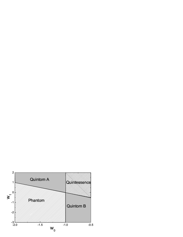
Moreover, we also consider another phenomenological parametrization, namely, oscillating Quintom whose EoS oscillates with time and is allowed to cross the cosmological constant boundary:

$$w_{\mathrm{DE}}(a)=w_{0}+w_{1}\sin(w_{2}\ln(a))~{}.$$ (7)

This oscillating behavior in EoS can lead to the oscillation on the Hubble diagram Xia:2006rr or a recurrent universe which can unify the early inflation and the current acceleration of our Universe Feng:2004ff . In Refs.Barenboim:2004kz ; Xia:2004rw ; Xia:2006rr ; Zhao:2006qg some preliminary studies have been presented on this kind of dark energy model. From the latest SNIa paper Riess:2006fw , one can find some hints of oscillating behavior in their Fig.$10$ where they used a polynomial fitting. Our sine function has the advantage of preserving the oscillating feature of the dark energy EoS at high redshift measured by the CMB data. For simplicity and focusing on the study at lower redshift, we set $w_{2}$ to be $3\pi/2$ in order to allow the EoS to evolve more than one period within the redshift range of $z=0$ to $z=2$ where the SNIa data are most robust. We label the above two dark energy parameterizations (6) and (7) as Para I and Para II respectively throughout this paper.

When using the MCMC global fitting strategy to constrain the cosmological parameters, it is crucial to include Dark Energy perturbation. The conservation law of energy reads:

$$T^{\mu\nu}{}_{;\mu}=0~{},$$ (8)

where $T^{\mu\nu}$ is the energy-momentum tensor of dark energy and “;” denotes the covariant differentiation. Working in the conformal Newtonian gauge and normally setting the anisotropic stress perturbation of dark energy to be zero, one can derive the perturbation equations of dark energy as follows ma :

$$\delta^{\prime} = -(1+w)(\theta-3\Phi^{\prime})-3\mathcal{H}(\hat{c}_{s}^{2}-w)\delta-3\mathcal{H}(w^{\prime}+3\mathcal{H}(1+w)(\hat{c}_{s}^{2}-w))\frac{\theta}{k^{2}}~{},$$ (9)

$$\theta^{\prime} = -\mathcal{H}(1-3\hat{c}_{s}^{2})\theta+k^{2}(\frac{\hat{c}_{s}^{2}\delta}{{1+w}}+\Psi)~{}.$$ (10)

However one cannot handle the Dark Energy perturbation when the parameterized EoS crosses $-1$ based on the Quintessence, Phantom, K-essence and other non-crossing dark energy models. By the virtue of Quintom dark energy model, the perturbation at the crossing points is continuous, thus we introduce a small positive constant $\epsilon$ to divide the full range of the allowed value of $w$ into three parts: 1) $w>-1+\epsilon$; 2) $-1+\epsilon\geq w\geq-1-\epsilon$; and 3) $w<-1-\epsilon$. Neglecting the entropy perturbation contributions, for the regions 1) and 3) the equation of state does not get across $-1$ and the perturbations are well defined by solving Eqs.(9,10). For the case 2), the density perturbation $\delta$ and velocity perturbation $\theta$, and the derivatives of $\delta$ and $\theta$ are finite and continuous for the realistic Quintom dark energy models. However for the perturbations of the parameterized EoS there is clearly a divergence. In our study for such a regime, we match the perturbation in region 2) to the regions 1) and 3) at the boundary and set:

$$\delta^{\prime}=0~{}~{},~{}~{}\theta^{\prime}=0~{}~{}.$$ (11)

In our numerical calculations we have limited the range to be $|\epsilon|<10^{-5}$ and we find our method is a very good approximation to the multi-field Quintom DE model. In our calculation the initial condition we choose is the adiabatic perturbations of dark energy, while the isocurvature perturbation of dark energy can be safely neglected Zhao:2005vj . For more details of this method we refer the readers to our previous companion papers Zhao:2005vj ; Xia:2005ge .

In our calculations we have taken the total likelihood to be the products of the separate likelihoods (${\bf\cal{L}}_{i}$) of CMB, LSS and SNIa. In other words defining $\chi_{L,i}^{2}\equiv-2\log{\bf\cal{L}}_{i}$, we get

$$\chi^{2}_{L,total}=\chi^{2}_{L,CMB}+\chi^{2}_{L,LSS}+\chi^{2}_{L,SNIa}~{}.$$ (12)

If the likelihood function is Gaussian, $\chi^{2}_{L}$ coincides with the usual definition of $\chi^{2}$ up to an additive constant corresponding to the logarithm of the normalization factor of ${\cal L}$. In the computation of CMB we have included the three-year WMAP (WMAP3) Temperature-Temperature (TT) and Temperature-Polarization (TE) power spectrum with the routine for computing the likelihood supplied by the WMAP team wmap3:2006:1 ; wmap3:2006:2 ; wmap3:2006:3 ; wmap3:2006:4 as well as the smaller scale experiments, including Boomerang-2K2 MacTavish:2005yk , CBI Readhead:2004gy , VSA Dickinson:2004yr and ACBAR Kuo:2002ua . For the Large Scale Structure information, we have used the Sloan Digital Sky Survey (SDSS) luminous red galaxy (LRG) sample Tegmark:2006az and 2dFGRS Cole:2005sx . To be conservative but more robust, in the fittings to the SDSS LRG sample we have used the first $15$ bins only, which are supposed to be well within the linear regime. In the calculation of the likelihood from SNIa we have marginalized over the nuisance parameter DiPietro:2002cz . The supernova data we use are the recently released ESSENCE (192 sample) data Miknaitis:2007jd ; Davis:2007na . Furthermore, we make use of the Hubble Space Telescope (HST) measurement of the Hubble parameter $H_{0}\equiv 100$h km s^-1 Mpc^-1 Hubble by multiplying the likelihood by a Gaussian likelihood function centered around $h=0.72$ and with a standard deviation $\sigma=0.08$. We also impose a weak Gaussian prior on the baryon density $\Omega_{b}h^{2}=0.022\pm 0.002$ (1 $\sigma$) from the Big Bang Nucleosynthesis BBN . Simultaneously we will also use a cosmic age tophat prior as 10 Gyr $<t_{0}<$ 20 Gyr.

For each regular calculation, we run 8 independent chains comprising of $150,000-300,000$ chain elements and spend thousands of CPU hours to calculate on a supercomputer. The average acceptance rate is about $40\%$. We test the convergence of the chains by Gelman and Rubin criteriaR-1 and find $R-1$ is of order $0.01$ which is more conservative than the recommended value $R-1<0.1$.

III Future Measurements

When considering the constraints on the cosmological parameters from the simulated data of future CMB (PLANCK and CMBpol) measurements, the fiducial models are obtained by maximizing the likelihood (the best-fit model) using the current observations.

Firstly we derive the likelihood function for a CMB experiment as given by Ref.Easther:2004vq ; Perotto:2006rj . Assuming the CMB multipoles are Gaussian distributed, one can obtain the likelihood function as follows:

$$\mathcal{L}\propto\prod_{lm}\frac{\exp\left[-\frac{1}{2}D^{{\dagger}}_{lm}C^{-1}D_{lm}\right]}{\sqrt{\det C}}~{},$$ (13)

where $D_{lm}=\left[a^{T}_{lm},a^{E}_{lm},a^{B}_{lm}\right]$ is the data vector of spherical harmonic coefficients which are contributed from the CMB signal $s_{lm}$ and the experimental noise $n_{lm}$: $a^{X}_{lm}=s^{X}_{lm}+n^{X}_{lm}$, and $C$ is the theoretical data covariance matrix generally given by:

$$C=\left(\begin{array}[]{ccc}\bar{C}^{TT}_{l}&\bar{C}^{TE}_{l}&\bar{C}^{TB}_{l}\\ \bar{C}^{TE}_{l}&\bar{C}^{EE}_{l}&\bar{C}^{EB}_{l}\\ \bar{C}^{TB}_{l}&\bar{C}^{EB}_{l}&\bar{C}^{BB}_{l}\\ \end{array}\right)=\left(\begin{array}[]{ccc}C^{TT}_{l}+N^{TT}_{l}&C^{TE}_{l}&C^{TB}_{l}\\ C^{TE}_{l}&C^{EE}_{l}+N^{EE}_{l}&C^{EB}_{l}\\ C^{TB}_{l}&C^{EB}_{l}&C^{BB}_{l}+N^{BB}_{l}\\ \end{array}\right)~{}.$$ (14)

In this covariance matrix, $C^{XX^{\prime}}_{l}$ denotes the theoretical power spectra and $N^{XX^{\prime}}_{l}$ is the noise power spectra which can be approximated as:

$$N^{XX^{\prime}}_{l}\equiv\langle n^{X{\dagger}}_{lm}n^{X^{\prime}}_{lm}\rangle=\delta_{XX^{\prime}}\theta^{2}_{{\mathrm{fwhm}}}\Delta^{2}_{X}\exp\left[l(l+1)\frac{\theta^{2}_{{\mathrm{fwhm}}}}{8\ln 2}\right]~{},$$ (15)

where $\theta_{{\mathrm{fwhm}}}$ is the full width at half maximum of the Gaussian beam, and $\Delta_{X}$ is the root mean square of the instrumental noise. Non-diagonal noise terms are expected to be zero since the noise contributions from different maps are uncorrelated. Due to the global isotropy, the terms $C^{TB}_{l}$ and $C^{EB}_{l}$ are always set to be zero. In our calculations we also assume them to be zero except for studying the possible CPT violation in the later section IV.3.

On the other hand, we can estimate the power spectra from the data as follows:

$$\hat{C}^{XY}_{l}=\sum_{m}\frac{|a^{X{\dagger}}_{lm}a^{Y}_{lm}|}{2l+1}~{}.$$ (16)

So we can obtain the effective $\chi^{2}_{{\mathrm{eff}}}$:

$$\chi^{2}_{{\mathrm{eff}}}\equiv-2\ln\mathcal{L}=\sum_{l}(2l+1)f_{{\mathrm{sky}}}\left(\frac{A}{|\bar{C}|}+\ln\frac{|\bar{C}|}{|\hat{C}|}+3\right)~{},$$ (17)

where $f_{{\mathrm{sky}}}$ denotes the observed fraction of the sky in the real experiments, $A$ is defined as:

$$A = \hat{C}^{TT}_{l}(\bar{C}^{EE}_{l}\bar{C}^{BB}_{l}-(\bar{C}^{EB}_{l})^{2})+\hat{C}^{TE}_{l}(\bar{C}^{TB}_{l}\bar{C}^{EB}_{l}-\bar{C}^{TE}_{l}\bar{C}^{BB}_{l})+\hat{C}^{TB}_{l}(\bar{C}^{TE}_{l}\bar{C}^{EB}_{l}-\bar{C}^{TB}_{l}\bar{C}^{EE}_{l})$$ (18)

$$+ \hat{C}^{TE}_{l}(\bar{C}^{TB}_{l}\bar{C}^{EB}_{l}-\bar{C}^{TE}_{l}\bar{C}^{BB}_{l})+\hat{C}^{EE}_{l}(\bar{C}^{TT}_{l}\bar{C}^{BB}_{l}-(\bar{C}^{TB}_{l})^{2})+\hat{C}^{EB}_{l}(\bar{C}^{TE}_{l}\bar{C}^{TB}_{l}-\bar{C}^{TT}_{l}\bar{C}^{EB}_{l})$$

$$+ \hat{C}^{TB}_{l}(\bar{C}^{TE}_{l}\bar{C}^{EB}_{l}-\bar{C}^{EE}_{l}\bar{C}^{TB}_{l})+\hat{C}^{EB}_{l}(\bar{C}^{TE}_{l}\bar{C}^{TB}_{l}-\bar{C}^{TT}_{l}\bar{C}^{EB}_{l})+\hat{C}^{BB}_{l}(\bar{C}^{TT}_{l}\bar{C}^{EE}_{l}-(\bar{C}^{TE}_{l})^{2})~{},$$

and $|\bar{C}|$ and $|\hat{C}|$ denote the determinants of the theoretical and observed data covariance matrices respectively,

$$|\bar{C}| = \bar{C}^{TT}_{l}\bar{C}^{EE}_{l}\bar{C}^{BB}_{l}+2\bar{C}^{TE}_{l}\bar{C}^{TB}_{l}\bar{C}^{EB}_{l}-\bar{C}^{TT}_{l}(\bar{C}^{EB}_{l})^{2}-\bar{C}^{EE}_{l}(\bar{C}^{TB}_{l})^{2}-\bar{C}^{BB}_{l}(\bar{C}^{TE}_{l})^{2}~{},$$ (19)

$$|\hat{C}| = \hat{C}^{TT}_{l}\hat{C}^{EE}_{l}\hat{C}^{BB}_{l}+2\hat{C}^{TE}_{l}\hat{C}^{TB}_{l}\hat{C}^{EB}_{l}-\hat{C}^{TT}_{l}(\hat{C}^{EB}_{l})^{2}-\hat{C}^{EE}_{l}(\hat{C}^{TB}_{l})^{2}-\hat{C}^{BB}_{l}(\hat{C}^{TE}_{l})^{2}~{}.$$ (20)

The likelihood has been normalized with respect to the maximum likelihood $\chi^{2}_{{\mathrm{eff}}}=0$, where $\bar{C}^{XY}_{l}=\hat{C}^{XY}_{l}$. If we set the ${C}^{TB}_{l}$ and ${C}^{EB}_{l}$ to be zero, the likelihood function will be reduced to the Eq.($17$) of Ref.Easther:2004vq . Furthermore, we can obtain the Eq.($9$) of Ref.Xia:2006wd if we ignore the tensor information.

In some of our simulations we also consider the gravitational lensing effect on the CMB power spectrum. The lensed Stokes parameters $I$, $Q$ and $U$ which specify the intensity and linear polarization of observed CMB are related to the unlensed Stokes parameters at the last scattering surface (denoted with a tilde) by $X(\textbf{n})=\tilde{X}(\textbf{n}^{\prime})=\tilde{X}(\textbf{n}+\delta\textbf{n})$, where $X$ denotes $I$, $Q$ or $U$ and $\delta\textbf{n}$ is the angular excursion of the photon as it propagates from the last scattering surface until the present. This deflection angle, $\delta\textbf{n}$, is given by the gradient of the lensing potential $\bigtriangledown\phi(\textbf{n})$,

$$\phi(\textbf{n})=2\int dr\frac{r-r_{s}}{rr_{s}}\Psi(r\hat{\textbf{n}},r)~{},$$ (21)

where $r$ is the comoving distance along the line of sight, $s$ denotes the CMB last scattering surface, and $\Psi$ is the three dimensional gravitational potential Zaldarriaga:1998ar ; Lewis:2006fu .

The important feature is that the gravitational lensing can mix $E$ and $B$ modes Zaldarriaga:1998ar . If we assume that there is only unlensed $E$ type polarization and the unlensed $\tilde{C}_{l}^{BB}=0$ in the last scattering surface, the gravitational lensing will generate $B$ type polarization in the observed field, $C_{l}^{BB}\neq 0$. The information from the gravitational lensing is added through the power spectrum for the lensing potential $C_{l}^{\phi\phi}$ and the correlation to the temperature $C_{l}^{T\phi}$:

$$\langle a^{\phi{\dagger}}_{lm}a^{\phi}_{l^{\prime}m^{\prime}}\rangle=(C_{l}^{\phi\phi}+N_{l}^{\phi\phi})\delta_{ll^{\prime}}\delta_{mm^{\prime}}~{}~{},~{}~{}\langle a^{T{\dagger}}_{lm}a^{\phi}_{l^{\prime}m^{\prime}}\rangle=(C_{l}^{T\phi}+N_{l}^{T\phi})\delta_{ll^{\prime}}\delta_{mm^{\prime}}~{},$$ (22)

which can be computed numerically in the linear theory using CAMB Lewis:1999bs . In our analysis we use the unlensed power spectra, $\tilde{C}_{l}^{TT}$, $\tilde{C}_{l}^{TE}$, $\tilde{C}_{l}^{EE}$, and $C_{l}^{\phi\phi}$, $C_{l}^{T\phi}$. We do not use the lensed power spectra to avoid the complication of the correlation in their errors between different $l$ values and with the error in $C_{l}^{\phi\phi}$ and $C_{l}^{T\phi}$ Hu:2001fb ; Smith:2006nk . For errors on $C_{l}^{\phi\phi}$ we follow the Ref.Hu:2001kj . We use the publicly available code Perotto:2006rj to simulate the mock CMB power spectra of our fiducial models. In Table I we list the assumed experimental specifications of the future Planck and CMBpol measurements and neglect the foreground contamination.

TABLE I. Assumed experimental specifications. We use the CMB power spectra only at $l\leq 2500$. The noise parameters $\Delta_{T}$ and $\Delta_{P}$ are given in units of $\mu$K-arcmin.

Experiment	$f_{\mathrm{sky}}$	$l_{\mathrm{max}}$	(GHz)	$\theta_{\mathrm{fwhm}}$	$\Delta_{T}$	$\Delta_{P}$
PLANCK	0.65	2500	100	9.5’	6.8	10.9
			143	7.1’	6.0	11.4
			217	5.0’	13.1	26.7
CMBpol	0.65	2500	217	3.0’	1.0	1.4

To make our constraints more robust, we add the simulated SNAP data to do all the simulations throughout this paper. The projected satellite SNAP (Supernova/Acceleration Probe) would be a space-based telescope with a one square degree field of view with $10^{9}$ pixels. It aims to increase the discovery rate for SNIa to about $2000$ per year. The simulated SNIa data distribution is taken from Refs.kim ; Li:2005zd . As for the error, we follow the Ref.kim which takes the magnitude dispersion $0.15$ and the systematic error $\sigma_{{\mathrm{sys}}}=0.02\times z/1.7$, and the whole error for each data is as follows:

$$\sigma_{{\mathrm{mag}}}(z_{i})=\sqrt{\sigma^{2}_{{\mathrm{sys}}}(z_{i})+\frac{0.15^{2}}{n_{i}}}~{},$$ (23)

where $n_{i}$ is the number of supernova in the $i^{\prime}$th redshift bin.

IV Results

In this section we show our global fitting results of the cosmological parameters and focus on the dark energy parameters, inflationary parameters, space-time curvature, total neutrino mass and the rotation angle denoting the possible CPT violation respectively.

IV.1 Equation of State of Dark Energy

TABLE II. Constraints on the EoS of dark energy and some background parameters from the current observations and the future simulations. Note that Para I and Para II represent $w_{\mathrm{DE}}(a)=w_{0}+w_{1}(1-a)$ and $w_{\mathrm{DE}}(a)=w_{0}+w_{1}\sin(3\pi/2\ln(a))$ respectively. For the current constraints we have shown the mean values $1,2\sigma$ (Mean) and the best fit results together. And we also list the standard deviation (SD) of these parameters based on the future simulations.

	$\Lambda$CDM			Para I			Para II
	Current		Future	Current		Future	Current
	Best Fit	Mean	SD	Best Fit	Mean	SD	Best Fit	Mean
$w_{0}$	$-1$	$-1$	$-$	$-1.16$	$-1.03^{+0.15+0.36}_{-0.15-0.26}$	$0.045$	$-0.898$	$-0.981^{+0.320+0.534}_{-0.340-0.748}$
$w_{1}$	$0$	$0$	$-$	$0.968$	$0.405^{+0.562+0.781}_{-0.587-1.570}$	$0.11$	$0.047$	$-0.068^{+0.561+1.037}_{-0.591-1.245}$
$~{}\Omega_{{\mathrm{DE}}}~{}$	$0.760$	$0.762^{+0.015+0.029}_{-0.015-0.033}$	$0.0043$	$0.756$	$0.760^{+0.017+0.033}_{-0.018-0.035}$	$0.0064$	$0.765$	$0.764^{+0.019+0.045}_{-0.019-0.044}$
$H_{0}$	$73.1$	$73.3^{+1.6+3.2}_{-1.7-3.2}$	$0.44$	$70.3$	$71.2^{+2.3+4.6}_{-2.3-4.2}$	$0.76$	$72.0$	$72.2^{+2.8+5.0}_{-2.6-6.3}$

To study the dynamics of dark energy, we parameterize our universe as follows:

$${\bf P}\equiv(\omega_{b},\omega_{c},\Theta_{s},\tau,w_{0},w_{1},n_{s},\log[10^{10}A_{s}])~{}.$$ (24)

Our main results of dark energy parameters are summarized in Table II. Besides the two parameterizations Para I and Para II, we also investigate the $\Lambda$CDM model for comparison. In addition, we present the future constraints for the $\Lambda$CDM model and Para I using the simulated Planck and SNAP data as introduced above. Marginalized over other cosmological parameters, in Table II we list the constraints on the dark energy parameters as well as the Hubble constant in different dark energy models.

Figure 2: Constraints on the dark energy parameters $w_{0}$ and $w_{1}$ from the combination of current observations (Black Solid Lines) and the future simulation data (Red Dashed Lines) respectively. The left panel is for Para I: $w_{{\mathrm{DE}}}(a)=w_{0}+w_{1}(1-a)$. And the right panel is for Para II: $w_{{\mathrm{DE}}}(a)=w_{0}+w_{1}\sin(\frac{3\pi}{2}\log(a))$. The two blue dotted lines in the ($w_{0},w_{1}$) panel distinguish the dark energy models and their intersecting point denotes the $\Lambda$CDM model.

Figure 3: Constraints on $w_{{\mathrm{DE}}}(a)=w_{0}+w_{1}(1-a)$ from the current observations. Median value (central red solid line), $68\%$ (inner, dark shaded area) and $95\%$ (outer, light shaded area) intervals are shown. The blue dashed lines denote the cosmological constant boundary.

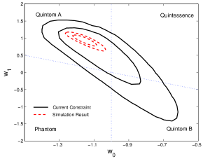
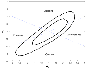
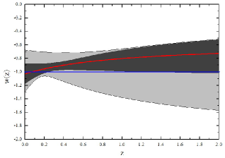
In Fig.2 we illustrate the constraints on the dark energy parameters $w_{0}$ and $w_{1}$ of two parameterizations. From the current observations we find that $w_{0}=-1.03\pm 0.15$, $w_{1}=0.405^{+0.562}_{-0.587}$ for Para I and the Quintom scenario, where $w(z)$ can cross the cosmological constant boundary during the evolution, is mildly favored. Using the current data, we find that the best fit model is located in the Quintom A region while the $\Lambda$CDM, denoted by the intersect of two straight lines, lies at the edge of $1\sigma$ contour. The one dimensional constraint on the evolution of $w(a)$ from the current data is shown in Fig.3. This behavior can be found more obviously from the best fit model. However, current data can not distinguish different dark energy models decisively, namely, the variance of $w_{0}$ and $w_{1}$ are too large to distinguish dynamical dark energy models from the $\Lambda$CDM model. The $\Lambda$CDM model is still a good fit right now.

In order to distinguish different Dark Energy models we consider the future measurements Planck and SNAP. The fiducial model we choose is the best fit model from the current constraints of Para I. We show the $68\%$ and $95\%$ confidence level contours (Red Dashed lines) on the left panel of Fig.2. As we expected, the constraints from the simulated data are much more stringent than the current constraints. By the virtue of Planck and SNAP data, we see that the standard deviations of $w_{0}$ and $w_{1}$ are $\sigma=0.045$ and $\sigma=0.11$ respectively, which are reduced by a factor of $3.33$ and $5.2$. The Quintom model and the $\Lambda$CDM model might be distinguished at around $4\sigma$ confidence level.

For Para II, the mean values from the current observations are $w_{0}=-0.981^{+0.320}_{-0.340}$, $w_{1}=-0.068^{+0.561}_{-0.591}$ which still support the Quintom scenario despite of the weak significance. In right panel of Fig.2, we see that the Quintom models occupies the most of the contour while the $\Lambda$CDM model still lies well within $1\sigma$ contour.

IV.2 Other Cosmological Parameters

The dynamics of dark energy can have profound effects on the determination of other cosmological parameters, such as the inflationary parameters ($n_{s}$, $\alpha_{s}$, $r$), the total neutrino mass $\sum m_{\nu}$ as well as the curvature of space-time $\Omega_{k}$, due to the well-known degeneracies among these parameters. In this subsection, we measure the above parameters in the framework of dynamical dark energy models.

TABLE III. Constraints on some cosmological parameters $n_{s}$, $\alpha_{s}$, $r$, $\Omega_{k}$ and $\sum m_{\nu}$ from the current observations and the future simulations. We have shown the mean $1,2\sigma$ errors (Mean) for the current constraints and the standard deviation (SD) of these parameters based on the future simulations. For the weakly constrained parameters we quote the $95\%$ upper limit instead.

	$\Lambda$CDM		Para I		Para II
	Mean	SD	Mean	SD	Mean
$n_{s}$	$0.953^{+0.014+0.028}_{-0.013-0.026}$	$0.003$	$0.965^{+0.017+0.038}_{-0.017-0.032}$	$0.0037$	$0.962^{+0.016+0.036}_{-0.017-0.031}$
$100\times\alpha_{s}$	$-3.75^{+2.19+4.24}_{-2.21-4.23}$	$0.53$	$-3.38^{+2.52+4.80}_{-2.50-4.76}$	$0.55$	$-3.95^{+2.37+4.86}_{-2.39-4.72}$
$r$	$<0.231$ ($95\%$)	$<0.055$ ($95\%$)	$<0.392$ ($95\%$)	$<0.074$ ($95\%$)	$<0.356$ ($95\%$)
$100\times\Omega_{k}$	$-0.873^{+0.788+1.454}_{-0.753-1.581}$	$0.289$	$-0.201^{+1.46+2.74}_{-1.29-2.58}$	$1.05$	$-0.593^{+1.23+3.51}_{-1.35-2.57}$
$\sum m_{\nu}$	$<0.958$ ($95\%$)	$0.077$	$<1.59$ ($95\%$)	$0.179$	$<1.53$ ($95\%$)

IV.2.1 Inflationary Models

The current acceleration and the inflation, the two stages of accelerated expansion of our universe, might have some deep relationship albeit the significant difference of energy scale between them. Some efforts have been made to unify these two expansion epoches, such as the quintessential inflation Pvilenkin . Moreover, the isocurvature perturbations in dark energy sector generated during inflation may give rise to the suppression of power of CMB at large scale, which can be mimicked by suppressed primordial spectrum Moroi:2003pq . This means different dynamics of the dark energy and inflation can lead to similar effects on observations and studying such degeneracies might unveil the possible connections between dark energy and inflation.

Figure 4: $1D$ current constraints on the parameters $n_{s}$, $\alpha_{s}$ and $r$ based on the different dark energy models: $\Lambda$CDM (black solid line), $w_{{\mathrm{DE}}}=w_{0}+w_{1}(1-a)$ (red dashed line) and $w_{{\mathrm{DE}}}=w_{0}+w_{1}\sin(\frac{3\pi}{2}\log(a))$ (blue dotted line).

In this section, we constrain the inflationary parameters in the framework of dynamical dark energy using the current and simulated datasets. We sample in the following 10 dimensional parameter space using MCMC algorithm:

$${\bf P}\equiv(\omega_{b},\omega_{c},\Theta_{s},\tau,w_{0},w_{1},n_{s},\log[10^{10}A_{s}],\alpha_{s},r)~{}.$$ (25)

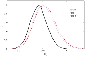
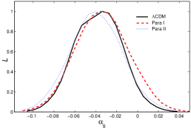
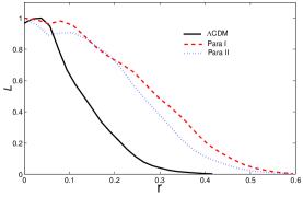
It’s noteworthy that we do not constrain $\alpha_{s}$ and $r$ simultaneously in our global fittings. From Table III, we can see the effects of dynamical dark energy on the determination of the inflationary parameters. Again, we give the fitting results for Para I, Para II and the $\Lambda$CDM model for comparison. We find that the constraints for the spectral index $n_{s}$, the running $\alpha_{s}$ and the tensor-to-scalar ratio $r$ have been weaken with the presence of dynamics of dark energy. Quantitatively, the $2\sigma$ constraints of $n_{s}$, $\alpha_{s}$ and $r$ can be relaxed by roughly $36\%$, $13\%$ and $70\%$ respectively. This can be seen from the one dimensional distribution plot of Fig.4.

The WMAP group found that the scale invariant primordial spectrum and the inflation models with $n_{s}>1$ is disfavored at almost the $3\sigma$ level. Our result is in good agreement with them, $n_{s}=0.953^{+0.014}_{-0.013}$, based on the $\Lambda$CDM model. However, we find that the mean value of $n_{s}$ moves toward to the “blue” spectral in the framework of dynamical dark energy model, $n_{s}=0.965\pm 0.017$. From the future data we find that the standard deviation of $n_{s}$ can be shrink to be $\sigma=0.003$ and the scale invariant spectrum will be verified with much higher confidence level.

Figure 5: $68\%$ and $95\%$ constraints on the panel ($n_{s}$, $r$) based on the different Dark Energy models: $\Lambda$CDM (black solid line), $w_{{\mathrm{DE}}}=w_{0}+w_{1}(1-a)$ (red dashed line) and $w_{{\mathrm{DE}}}=w_{0}+w_{1}\sin(\frac{3\pi}{2}\log(a))$ (blue dotted line). The two solid green lines delimit the three classes of inflation models, namely, small-field, large-field and hybrid models. The blue points are predicted by $m^{2}\phi^{2}$ model and $\lambda\phi^{4}$ model respectively. These predictions assume that the number of e-foldings, $N$, is $50-60$ for $m^{2}\phi^{2}$ model and $64$ for $\lambda\phi^{4}$ model. The magenta dash-dotted lines denote the $1,2\sigma$ contours obtained from the future simulated data.

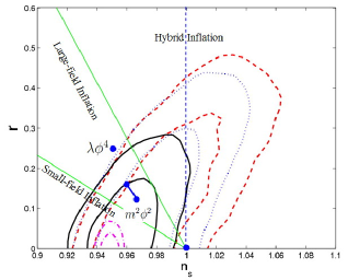
In the framework of dynamical dark energy model, from Fig.4, we find that the $95\%$ upper limit of $r$ can be relax from $r<0.231$ to $r<0.392$. The degeneracy may be due to the reason that the tensor fluctuation and the dark energy component mostly affect the large scale (low multipoles) power spectrum of CMB. In the two dimensional plot of Fig.5, we find that the Harrison-Zel’dovich-Peebles scale invariant (HZ) spectrum ($n_{s}=1,~{}r=0$) is disfavored about $2\sim 3\sigma$ in $\Lambda$CDM model. However, this spectrum can be allowed with the presence of the dynamics of dark energy. The single slow-rolling scalar field with potential $V(\phi)\sim m^{2}\phi^{2}$, which predicts $(n_{s},r)=(1-2/N,8/N)$, is well within $1\sigma$ region, while another single slow-rolling scalar field with potential $V(\phi)\sim\lambda\phi^{4}$, which predicts $(n_{s},r)=(1-3/N,12/N)$, is excluded about $2\sigma$ in the $\Lambda$CDM model. Interestingly many hybrid inflation models, excluded in the $\Lambda$CDM model, revive in the framework of dynamical dark energy model as illustrated in Fig.5.

Another feature of WMAP data, both for WMAP1 peiris and WMAP3 wmap3:2006:1 ; Easther:2006tv , is the large running of the scalar primordia spectrum index $\alpha_{s}$. Our result shows that the large running is favored more than $1\sigma$, $\alpha_{s}=-0.038\pm 0.022$. In Fig.4 we find that the dynamical dark energy models enlarge the error of $\alpha_{s}$ slightly and do not affect the mean value obviously.

Given the large uncertainties in the constraints of inflationary parameters from the current observations, different inflation models cannot be distinguished conclusively. Yet, the constraints from the future Planck measurement can make this possible. From our simulation results in Table III, we find that the error bars of inflationary parameters can be reduced by about a factor of $5$. This dramatic improvement will play a crucial role in the study of dynamics of inflation and can also shed light on the investigate of the dynamical dark energy model due to the correlations among inflationary and dark energy parameters.

IV.2.2 Curvature of Universe

Dark energy and the curvature, $\Omega_{K}=1-\Omega_{m}-\Omega_{{\mathrm{DE}}}$, are dominant factors in determining the fate of our Universe. Further, DE parameters and $\Omega_{K}$ are correlated. This is expected since $\Omega_{K}$ and dark energy can contribute to the luminosity distance $d_{L}$ via:

$$d_{\rm L}(z) = \frac{1+z}{H_{0}\sqrt{|\Omega_{k}|}}{\rm sinn}\left[\sqrt{|\Omega_{k}|}\int_{0}^{z}\frac{dz^{\prime}}{E(z^{\prime})}\right]~{},$$ (26)

$$E(z)\equiv\frac{H(z)}{H_{0}} = \sqrt{\Omega_{m}(1+z)^{3}+\Omega_{{\mathrm{DE}}}\exp\left(3\int_{0}^{z}\frac{1+w(z^{\prime})}{1+z^{\prime}}dz^{\prime}\right)+\Omega_{K}(1+z)^{2}}~{},$$ (27)

where ${\rm sinn}(\sqrt{|k|}x)/\sqrt{|k|}=\sin(x)$, $x$, $\sinh(x)$ if $k<0$, $k=0$ and $k>0$. In addition, $\Omega_{K}$ can modify the angular diameter distance to last scattering surface, which leaves imprints on the CMB power spectrum.

Figure 6: $1D$ current constraints on the parameters $\Omega_{k}$ based on the different dark energy models: $\Lambda$CDM (black solid line), $w_{{\mathrm{DE}}}=w_{0}+w_{1}(1-a)$ (red dashed line) and $w_{{\mathrm{DE}}}=w_{0}+w_{1}\sin(\frac{3\pi}{2}\log(a))$ (blue dotted line).

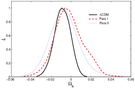
We concentrate on the determination of $\Omega_{K}$ in dynamical dark energy models using current and simulated data. Our parameter space is:

$${\bf P}\equiv(\omega_{b},\omega_{c},\Omega_{k},\Theta_{s},\tau,w_{0},w_{1},n_{s},\log[10^{10}A_{s}])~{}.$$ (28)

From Table III and Fig.6, we see our universe is very close to flatness, namely, the absolute value of space-time curvature $|\Omega_{k}|$ is smaller than $0.025$ in the $\Lambda$CDM model, $0.028$ for Para I and $0.032$ for Para II. The dynamics of dark energy weakens the constraint of $|\Omega_{k}|$ due to the well-known correlation among $\Omega_{k}$ and dark energy parameters. This correlation plays a crucial role in the reconstruction of equation of state of dark energy Clarkson:2007bc . By the simulated data, we are able to detect the curvature more accurately.

IV.2.3 Neutrino Mass

Detecting the absolute mass of neutrino is another challenge of modern physics. The cosmological observations can obtain upper limits of the absolute neutrino mass. For background evolution, neutrino masses, albeit small, contribute to the cosmic energy budget and modify the epoch of matter-radiation equality, angular diameter distance to the last scattering surface and other related physical quantities. For the evolution of perturbation, neutrino becomes non-relativistic at late time thus they damp the perturbation within their free streaming scale. Thus the matter power spectrum can be suppressed by roughly $\Delta P/P\sim-8\Omega_{\nu}/\Omega_{m}$ Hu:1997mj . As a result, neutrino can leave imprints on the cosmological observations, such as CMB and matter power spectrum. On the other hand, the evolution of dark energy can also affect the evolution of background and perturbation, which mimics the behavior of neutrino to some extent. This leads to an obvious degeneracy among dark energy parameters and the neutrino mass.

The degeneracy between dark energy with constant equation of state and neutrino mass has been studied in the literature Hannestad:2005gj ; wmap3:2006:1 . In this section, we update our previous results to study the upper limits of neutrino mass with the presence of dynamical dark energy Xia:2006wd and investigate the degeneracy between dynamical dark energy and neutrino mass with current cosmological observations as well as with the future simulated data.

Figure 7: $1D$ current constraints on the parameters $\sum m_{\nu}$ based on the different dark energy models: $\Lambda$CDM (black solid line), $w_{{\mathrm{DE}}}=w_{0}+w_{1}(1-a)$ (red dashed line) and $w_{{\mathrm{DE}}}=w_{0}+w_{1}\sin(\frac{3\pi}{2}\log(a))$ (blue dotted line).

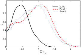
We concentrate on the determination of $\sum m_{\nu}$ in dynamical dark energy models using current and simulated data. Our parameter space is:

$${\bf P}\equiv(\omega_{b},\omega_{c},\Theta_{s},\tau,w_{0},w_{1},f_{\nu},n_{s},\log[10^{10}A_{s}])~{}.$$ (29)

In the last row of Table III, one can read $95\%~{}C.L.$ neutrino mass limits derived from the current observations as well as the simulated data of Planck and SNAP in the $\Lambda$CDM and dynamical dark energy models. In the $\Lambda$CDM model, the limit of neutrino mass we get, $\sum m_{\nu}<0.958~{}eV~{}(95\%)$, is consistent with Tegmark’s result Tegmark:2006az . For the dynamical dark energy model, the limit can be relaxed to $\sum m_{\nu}<1.59~{}eV~{}(95\%)$ and $\sum m_{\nu}<1.53~{}eV~{}(95\%)$ obviously, due to the degeneracy between the dark energy parameters and the neutrino mass from the geometric feature of our Universe Xia:2006wd ; Hannestad:2005gj . In Fig.7 we illustrate this effect with current astronomical data.

With the simulated data, we obtain the two tail posterior distribution due to the nonzero fiducial value of neutrino mass. The standard deviation will be greatly tightened to be $0.077~{}eV$. With the presence of dynamical dark energy, the standard deviation can be relaxed by a factor of $2.3$ using the simulated data. We might distinguish the normal hierarchy ($\sum m_{\nu}\sim 0.05~{}eV$) from the inverted hierarchy ($\sum m_{\nu}\sim 0.1~{}eV$) using the future Planck measurement.

IV.3 Cosmological CPT Violation

The CPT symmetry which has been proved to be exact within the framework of standard model of particle physics and Einstein gravity could be violated dynamically during the evolution of the universe Li:2006ss . The detection of CPT violation will reveal new physics beyond the standard model. In our previous work we studied the cosmological CPT violation in the photon sector. We introduce a Chern-Simons term in the effective Lagrangian of the form Carroll:1989vb :

$$\Delta\mathcal{L}=-\frac{1}{4}p_{\mu}A_{\nu}\tilde{F}^{\mu\nu}~{},$$ (30)

where $p_{\mu}$ is a four-vector and $\tilde{F}^{\mu\nu}=(1/2)\epsilon^{\mu\nu\rho\sigma}F_{\rho\sigma}$ is the dual of the electromagnetic tensor. This action is gauge invariant if $p_{\mu}$ is a constant and homogeneous vector or the gradient of a scalar. It violates Lorentz and CPT symmetries if the background value of $p_{\mu}$ is nonzero. In the scenario of quintessential baryo-/leptogenesis Li:2001st ; Li:2002wd the four-vector $p_{\mu}$ is in the form of the derivative of the quintessence scalar, $\partial_{\mu}\phi$. During the evolution of quintessence, the time component of $\partial_{\mu}\phi$ does not vanish, which causes CPT violation. In the scenario of gravitational baryo-/leptogenesis Davoudiasl:2004gf ; Li:2004hh , $p_{\mu}$ is the gradient of a function of Ricci scalar R.

Figure 8: $1D$ current constraints on the rotation angle $\Delta\alpha$ from the simulated Planck (Black Solid line) and CMBpol (Red Dahsed line) data.

The interaction in Eq.(30) violates also the P and CP symmetries, as long as $p_{0}$ does not vanish Klinkhamer:1999zh . It leads to a rotation of the polarization vector of electromagnetic waves when they are propagating over cosmological distances. This effect is known as “cosmological birefringence”. The polarization vector of each photon is rotated by an angle $\Delta\alpha$ and one would modify the power spectra of TE, EE, BB, TB and EB at the last scattering surface as:

$$C_{l}^{{}^{\prime}TB} = C_{l}^{TE}\sin(2\Delta\alpha)~{},$$ (31)

$$C_{l}^{{}^{\prime}EB} = \frac{1}{2}(C_{l}^{EE}-C_{l}^{BB})\sin(4\Delta\alpha)~{},$$ (32)

$$C_{l}^{{}^{\prime}TE} = C_{l}^{TE}\cos(2\Delta\alpha)~{},$$ (33)

$$C_{l}^{{}^{\prime}EE} = C_{l}^{EE}\cos^{2}(2\Delta\alpha)+C_{l}^{BB}\sin^{2}(2\Delta\alpha)~{},$$ (34)

$$C_{l}^{{}^{\prime}BB} = C_{l}^{BB}\cos^{2}(2\Delta\alpha)+C_{l}^{EE}\sin^{2}(2\Delta\alpha)~{},$$ (35)

where the primed quantities are rotated. In Ref.Feng:2006dp we have performed a global fit and found that a nonzero rotation angle of the photons is mildly favored, $\Delta\alpha=-6.0\pm 4.0$ deg, using the WMAP3 (without the information of TB and EB power spectra) and full data of Boomerang-2K2.

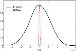
In Fig.8, by the simulated data with Planck and CMBpol accuracy, we find that the standard deviation of the rotation angle will be greatly tightened to $\sigma=0.057$ deg for PLANCK and $\sigma=2.57\times 10^{-3}$ deg for CMBpol. These results are much more stringent than the current constraint and will be used to verify the CPT symmetry with a higher precision Feng:2004mq .

V Summary

Since the mystery of our Universe encodes in the cosmological parameters, constraining these parameters with the latest observational data and doing error forecasts with the simulated futuristic data can lead us to understand the Nature. In this paper, we focus on the dynamics of dark energy in light of current and simulated Planck and SNAP data and then constrain the inflationary parameters, total neutrino mass and curvature of space-time in the framework of dynamical dark energy model. In addition, we investigate the rotation angle $\Delta\alpha$, the possible signature of CPT violation, by simulated Planck and CMBpol data.

Parameterizing the EoS of dark energy in two forms as Eqs.(6,7), we find that the Quintom model, whose EoS crosses $-1$ during the evolution, is mildly favored by latest observations, albeit the $\Lambda$CDM model remains a good fit. Using the simulated Planck data complimented by SNAP data, we find that the variance of the dark energy parameters in Eq.(6) decreases dramatically, namely, $\sigma(w_{0})$ and $\sigma(w_{1})$ can be reduced by a factor of $3.33$ and $5.2$ respectively. Given the current central value, this means that Planck can distinguish dynamical dark energy from the $\Lambda$CDM model at around 4$\sigma$ confidence level.

Since the dynamics of dark energy greatly affects the determination of other cosmological parameters, we constrain the inflationary parameters, total neutrino mass $\sum m_{\nu}$ and curvature of space-time $\Omega_{K}$ with the presence of dynamics of dark energy using current and simulated observational data. We find that the dynamics of dark energy generally weakens the determination of other cosmological parameters. For instance, we find that the inflation models with a “blue” tilt ($n_{s}>1$), which is strongly disfavored in the $\Lambda$CDM model, are now well within $2\sigma$ region in the framework of dynamical dark energy model. This is something intriguing in that Hybrid Inflation Models have been revived due to the dynamical dark energy, due to the obviously enlarged parameter space of ($n_{s}$,$r$) in the framework of dynamical dark energy model. These discoveries can lead us to further study the dynamics of inflation, dark energy and the relationship between them. With Planck, the uncertainties of inflationary parameters, including $n_{s},~{}\alpha_{s},~{}r$, can be roughly reduced by a factor of $5$. This significant improvement make it possible to distinguish the inflationary models decidedly.

The presence of dark energy can relax the upper limit of neutrino mass by a factor of $2$. This sheds new light on the research of neutrino physics, such as the scenario of mass varying neutrino mvn1 ; mvn2 . By Planck, we can rise the precision of measurement of this mass limit by a factor of $12$, namely, the standard deviation of neutrino mass can be shrunk to $0.077~{}eV$ for the $\Lambda$CDM model and $0.179~{}eV$ for the dynamical dark energy model (Para I). This measurement might make us understand the Nature of physics conclusively. Current data imply that our Universe is very close to flatness, say, $|\Omega_{K}|<0.03~{}(95\%~{}C.L.)$. By Planck, we can reduce $\sigma(\Omega_{K})$ by a factor of $2.67$($\Lambda$CDM). Such improvement helps us to reveal the Nature of space-time.

The global symmetry of CPT plays a critical role in understanding the fundamental physics. In our previous works we have found some hints of CPT violation encoded in the rotation angel of polarization vector of photons $\Delta\alpha$. With Planck and CMBpol, we can test the CPT symmetry at a unprecedent accuracy.

Acknowledgments: We acknowledge the use of the Legacy Archive for Microwave Background Data Analysis (LAMBDA). Support for LAMBDA is provided by the NASA Office of Space Science. We have performed our numerical analysis on the Shanghai Supercomputer Center (SSC). We are grateful to Laurence Perotto for discussions related to the simulation of lensed CMB power spectra. We thank Yi-Fu Cai, Zu-Hui Fan, Pei-Hong Gu, Steen Hannestad, Hiranya Peiris, Yun-Song Piao, Levon Pogosian, Tao-Tao Qiu and Douglas Scott for helpful discussions. This work is supported in part by National Natural Science Foundation of China under Grant Nos. 90303004, 10533010 and 10675136 and by the Chinese Academy of Science under Grant No. KJCX3-SYW-N2.

References

- (1) G. Miknaitis et al., arXiv:astro-ph/0701043.
- (2) T. M. Davis et al., arXiv:astro-ph/0701510.
- (3) D. N. Spergel et al., Astrophys. J. Suppl. 170, 377 (2007).
- (4) L. Page et al., Astrophys. J. Suppl. 170, 335 (2007).
- (5) G. Hinshaw et al., Astrophys. J. Suppl. 170, 288 (2007).
- (6) N. Jarosik et al., Astrophys. J. Suppl. 170, 263 (2007).
- (7) M. Tegmark et al., Phys. Rev. D 74, 123507 (2006).
- (8) B. Feng, M. Li, J. Q. Xia, X. Chen and X. Zhang, Phys. Rev. Lett. 96, 221302 (2006).
- (9) A. G. Riess et al., Astron. J. 116, 1009 (1998); S. Perlmutter et al., Astrophys. J. 517, 565 (1999).
- (10) S. Weinberg, Rev. Mod. Phys. 61, 1 (1989); I. Zlatev, L.-M. Wang, and P. J. Steinhardt, Phys. Rev. Lett. 82, 896 (1999).
- (11) B. Ratra and P. J. E. Peebles, Phys. Rev. D 37, 3406 (1988); P. J. E. Peebles and B. Ratra, Astrophys. J. 325, L17 (1988); C. Wetterich, Nucl. Phys. B 302, 668 (1988); C. Wetterich, Astron. Astrophys. 301, 321 (1995).
- (12) R. R. Caldwell, Phys. Lett. B 545, 23 (2002).
- (13) C. Armendariz-Picon, V. Mukhanov and P. J. Steinhardt, Phys. Rev. Lett. 85, 4438 (2000); Phys. Rev. D 63, 103510 (2001).
- (14) B. Feng, X. L. Wang and X. M. Zhang, Phys. Lett. B 607, 35 (2005).
- (15) J. Q. Xia, G. B. Zhao, B. Feng, H. Li and X. Zhang, Phys. Rev. D 73, 063521 (2006).
- (16) J. Q. Xia, G. B. Zhao, B. Feng and X. Zhang, JCAP 0609, 015 (2006).
- (17) G. B. Zhao, J. Q. Xia, B. Feng and X. Zhang, Int. J. Mod. Phys. D 16, 1229 (2007).
- (18) J. Q. Xia, G. B. Zhao and X. Zhang, Phys. Rev. D 75, 103505 (2007).
- (19) G. B. Zhao, J. Q. Xia, H. Li, C. Tao, J. M. Virey, Z. H. Zhu and X. Zhang, Phys. Lett. B 648, 8 (2007).
- (20) D. Huterer and A. Cooray, Phys. Rev. D 71, 023506 (2005); U. Alam, V. Sahni and A. A. Starobinsky, JCAP 0702, 011 (2007); V. Barger, Y. Gao and D. Marfatia, Phys. Lett. B 648, 127 (2007); H. Li, M. Su, Z. Fan, Z. Dai and X. Zhang, Phys. Lett. B 658, 95 (2008).
- (21) J. Q. Xia, Y. F. Cai, T. T. Qiu, G. B. Zhao and X. Zhang, arXiv:astro-ph/0703202.
- (22) A. Vikman, Phys. Rev. D 71, 023515 (2005).
- (23) M. Kunz and D. Sapone, Phys. Rev. D 74, 123503 (2006).
- (24) H. Wei and R. G. Cai, Class. Quant. Grav. 22, 3189 (2005); R. G. Cai, H. S. Zhang and A. Wang, Commun. Theor. Phys. 44, 948 (2005); A. A. Andrianov, F. Cannata and A. Y. Kamenshchik, Phys. Rev. D 72, 043531 (2005); X. Zhang, Int. J. Mod. Phys. D 14, 1597 (2005); Q. Guo and R. G. Cai, gr-qc/0504033; B. McInnes, Nucl. Phys. B 718, 55 (2005); E. Elizalde, S. Nojiri, S. D. Odintsov and P. Wang, Phys. Rev. D 71, 103504 (2005); I. Y. Aref’eva, A. S. Koshelev, and S. Yu. Vernov, Phys. Rev. D 72, 064017 (2005); A. Anisimov, E. Babichev and A. Vikman, J. Cosmol. Astropart. Phys. 0506, 006 (2005); H. Stefancic, Phys. Rev. D 71, 124036 (2005); J. Zhang, X. Zhang and H. Liu, arXiv:astro-ph/0612642.
- (25) A. H. Guth, Phys. Rev. D 23, 347 (1981); K. Sato, Mon. Not. Roy. Astron. Soc. 195, 467 (1981); For a review see e.g. A. D. Linde, Phys. Rept. 333, 575 (2000).
- (26) For relevant studies see also A. H. Guth and S. H. H. Tye, Phys. Rev. Lett. 44, 631 (1980) [Erratum-ibid. 44, 963 (1980)]; A. A. Starobinsky, Phys. Lett. B 91, 99 (1980).
- (27) R. Easther and H. Peiris, JCAP 0609, 010 (2006).
- (28) Planck Collaboration, arXiv:astro-ph/0604069.
- (29) G. B. Zhao, J. Q. Xia, M. Li, B. Feng and X. Zhang, Phys. Rev. D 72, 123515 (2005).
- (30) A. Lewis and S. Bridle, Phys. Rev. D 66, 103511 (2002).
- (31) A. Kosowsky and M. S. Turner, Phys. Rev. D 52, 1739 (1995); J. E. Lidsey, A. R. Liddle, E. W. Kolb, E. J. Copeland, T. Barreiro and M. Abney, Rev. Mod. Phys. 69, 373 (1997); S. Hannestad, S. H. Hansen, F. L. Villante and A. J. S. Hamilton, Astropart. Phys. 17, 375 (2002); S. L. Bridle, A. M. Lewis, J. Weller and G. Efstathiou, Mon. Not. Roy. Astron. Soc. 342, L72 (2003); B. Feng, X. Gong and X. Wang, Mod. Phys. Lett. A 19, 2377 (2004).
- (32) M. Chevallier and D. Polarski, Int. J. Mod. Phys. D 10, 213 (2001).
- (33) J. Q. Xia, G. B. Zhao, H. Li, B. Feng and X. Zhang, Phys. Rev. D 74, 083521 (2006).
- (34) B. Feng, M. Li, Y. S. Piao and X. Zhang, Phys. Lett. B 634, 101 (2006).
- (35) G. Barenboim, O. Mena and C. Quigg, Phys. Rev. D 71, 063533 (2005).
- (36) J. Q. Xia, B. Feng and X. M. Zhang, Mod. Phys. Lett. A 20, 2409 (2005).
- (37) A. G. Riess et al., arXiv:astro-ph/0611572.
- (38) C. P. Ma and E. Bertschinger, Astrophys. J. 455, 7 (1995).
- (39) C. J. MacTavish et al., Astrophys. J. 647, 799 (2006).
- (40) A. C. S. Readhead et al., Astrophys. J. 609, 498 (2004).
- (41) C. Dickinson et al., Mon. Not. Roy. Astron. Soc. 353, 732 (2004).
- (42) C. l. Kuo et al., Astrophys. J. 600, 32 (2004).
- (43) S. Cole et al., Mon. Not. Roy. Astron. Soc. 362 (2005) 505.
- (44) E. Di Pietro and J. F. Claeskens, Mon. Not. Roy. Astron. Soc. 341, 1299 (2003).
- (45) W. L. Freedman et al., Astrophys. J. 553, 47 (2001).
- (46) S. Burles, K. M. Nollett and M. S. Turner, Astrophys. J. 552, L1 (2001).
- (47) A. Gelman and D. Rubin, Statistical Science 7, 457 (1992).
- (48) R. Easther, W. H. Kinney and H. Peiris, JCAP 0505, 009 (2005).
- (49) L. Perotto, J. Lesgourgues, S. Hannestad, H. Tu and Y. Y. Y. Wong, JCAP 0610, 013 (2006).
- (50) M. Zaldarriaga and U. Seljak, Phys. Rev. D 58, 023003 (1998).
- (51) A. Lewis and A. Challinor, Phys. Rept. 429, 1 (2006).
- (52) A. Lewis, A. Challinor and A. Lasenby, Astrophys. J. 538, 473 (2000).
- (53) W. Hu, Phys. Rev. D 65, 023003 (2002).
- (54) K. M. Smith, W. Hu and M. Kaplinghat, Phys. Rev. D 74, 123002 (2006).
- (55) W. Hu and T. Okamoto, Astrophys. J. 574, 566 (2002).
- (56) A. G. Kim, E. V. Linder, R. Miquel and N. Mostek, Mon. Not. Roy. Astron. Soc. 347, 909 (2004).
- (57) H. Li, B. Feng, J. Q. Xia and X. Zhang, Phys. Rev. D 73, 103503 (2006).
- (58) P. J. E. Peebles and A. Vilenkin, Phys. Rev. D 59, 063505 (1999).
- (59) T. Moroi and T. Takahashi, Phys. Rev. Lett. 92, 091301 (2004).
- (60) H. V. Peiris et al., Astrophys. J. Suppl. 148, 213 (2003).
- (61) C. Clarkson, M. Cortes and B. A. Bassett, JCAP 0708, 011 (2007).
- (62) W. Hu, D. J. Eisenstein and M. Tegmark, Phys. Rev. Lett. 80, 5255 (1998).
- (63) S. Hannestad, Phys. Rev. Lett. 95, 221301 (2005).
- (64) M. Li, J. Q. Xia, H. Li and X. Zhang, Phys. Lett. B 651, 357 (2007).
- (65) S. M. Carroll, G. B. Field and R. Jackiw, Phys. Rev. D 41, 1231 (1990).
- (66) M. z. Li, X. l. Wang, B. Feng and X. m. Zhang, Phys. Rev. D 65, 103511 (2002).
- (67) M. Li and X. Zhang, Phys. Lett. B 573, 20 (2003).
- (68) H. Davoudiasl, R. Kitano, G. D. Kribs, H. Murayama and P. J. Steinhardt, Phys. Rev. Lett. 93, 201301 (2004).
- (69) H. Li, M. z. Li and X. m. Zhang, Phys. Rev. D 70, 047302 (2004).
- (70) F. R. Klinkhamer, Nucl. Phys. B 578, 277 (2000).
- (71) P. Cabella, P. Natoli and J. Silk, arXiv:0705.0810 [astro-ph].
- (72) J. Q. Xia, H. Li, X. l. Wang and X. m. Zhang, arXiv:0710.3325 [hep-ph].
- (73) B. Feng, H. Li, M. z. Li and X. m. Zhang, Phys. Lett. B 620, 27 (2005).
- (74) P. Gu, X. Wang and X. Zhang, Phys. Rev. D 68, 087301 (2003); R. Fardon, A. E. Nelson and N. Weiner, JCAP 0410, 005 (2004); R. D. Peccei, Phys. Rev. D 71, 023527 (2005).
- (75) G. B. Zhao, J. Q. Xia and X. M. Zhang, JCAP 0707, 010 (2007).