The Mirage of $w=-1$

Abstract

We demonstrate that cosmic microwave background observations consistent with a cosmological constant universe predict in a well-defined sense that lower redshift measures will nearly automatically deliver $w=-1$ for the dark energy equation of state value unless they are sensitive to $w(z)$. Thus low redshift data pointing to $w=-1$ does not truly argue for a cosmological constant. Even the simplest question of whether the equation of state of dark energy is equal to the cosmological constant therefore requires experiments able to sensitively constrain time variation $w(z)$ and not merely a constant $w$. We also note a number of issues regarding parametrization of $w(z)$, demonstrating that the standard form $w(z)=w_{0}+w_{a}z/(1+z)$ is robust but use of high order polynomials and cutting off the high redshift behavior can be pathological.

I Introduction

Advances in observational cosmology have led to tightening constraints on the properties of dark energy accelerating the cosmic expansion. Combinations of current data – Type Ia supernovae distances (SN) together with cosmic microwave background (CMB) fluctuations and galaxy surveys measuring baryon acoustic oscillation (BAO) scales – yield error bars on the effective pressure to energy density, or equation of state (EOS) ratio $w\approx-1\pm 0.1$ (e.g. kowal ). This represents significant progress in a first step toward checking consistency with a cosmological constant, possessing $w=-1$ at all redshifts.

The generation of experiments now and in the next few years achieves constraints in terms of a time independent EOS, which can also be thought of as an average over the range of observations, a substantial fraction of a Hubble expansion time. This article argues that such interpretation is very limited in providing new insight into dark energy, and will exhibit a definite tendency to deliver $w=-1$ despite real time variation. Therefore we should not consider experiments without specific sensitivity to time variation $w(z)$ as answering any questions about the nature of the accelerating universe. Rather, they serve crucial roles as technological and methodological developments, in particular for controlling systematic uncertainties.

Section II shows how the tendency arises that if CMB measurements of averaged dark energy influence implies $\langle w\rangle=-1$ then low redshift measurements will almost necessarily think $w=-1$. Since this does not imply that $w(z)=-1$, §III examines the robustness of parameterizing the high redshift behavior of $w(z)$. It is tempting to add more parameters to the EOS description, but §IV points out several pitfalls and pathologies in this approach, as well as when it partially succeeds.

The main purpose of this article is pedagogical emphasis on and clarification of the degeneracies and complementarity of different distance measures, and the essential need for experiments capable of precision measurements of the time variation of the equation of state, $w(z)$, before any real progress can be made in understanding the accelerating universe.

II Matching and Crossover

Distances, whether luminosity distances of SN or angular distances of the CMB or BAO, involve integrals of the Hubble parameter and its constituent energy densities and double integrals of the dark energy equation of state. This implies these quantities are intimately related and precise data in a distance will have implications for the allowed cosmological model parameters and density-redshift and EOS-redshift relations. More explicitly, one can derive a chain of physical conditions, where matching distances in two models (so as to agree with data) leads to a convergence at certain redshifts in the behavior of the energy densities and a crossover (equal values) in the EOS.

For example, francis noted that matching the reduced distance to CMB last scattering $d_{\rm lss}$ led to a convergence of the dark energy density ratio between two models and a crossover in $w(z)=w_{0}+w_{a}z/(1+z)$ at $a\approx 0.7$. Here we derive these relations analytically and investigate the implications for measurement of $w$.

Suppose we fix the distance to some redshift $z$ to be some value, say $d_{\rm lss}$ to that of a concordance cosmological constant (LCDM) cosmology with matter density $\Omega_{m}=0.234$, in agreement with the analysis of spergel . If we also hold the present matter density fixed (for the moment, we address its variation later) then we can derive a quantity

$$A = \int_{1}^{Y}dy\,\frac{\ln y}{(\Omega_{m}y^{3}+1-\Omega_{m})^{3/2}}$$ (1)

$$\Big{/}\int_{1}^{Y}dy\,\frac{\ln y+y^{-1}-1}{(\Omega_{m}y^{3}+1-\Omega_{m})^{3/2}},$$

where $Y=1+z$. The dark energy density of the model, $\Omega_{w}(z)$, will cross the curve of the fiducial dark energy density, e.g. $\Omega_{\Lambda}(z)$, at a crossover scale factor $a_{\Omega}$ solving

$$\frac{1-a_{\Omega}}{\ln a_{\Omega}}=A^{-1}-1.$$ (2)

Moreover, the dark energy EOS will cross $w=-1$ at a crossover scale factor

$$a_{w}=1-A^{-1}.$$ (3)

We see there is a definite relation between $a_{\Omega}$ and $a_{w}$. The $w=-1$ crossover is very robust. If we change the fiducial value of $\Omega_{m}$ from 0.2 to 0.35 then $a_{w}$ ranges from 0.707 to 0.733, while $a_{\Omega}$ goes from 0.476 to 0.518.

Thus a high redshift distance measurement consistent with LCDM virtually forces (within the picture so far) the value $w(z\approx 0.4)=-1$, irrespective of true time variation. However, low redshift measurements insufficiently sensitive to time variation measure only an averaged EOS that corresponds strongly to the value at a sweet spot or “pivot” redshift with the pivot near $z\approx 0.4$. That is, the averaged EOS will necessarily appear to be $w\approx-1$, despite the presence of varying $w(z)$. Not only is no new insight provided, but failing to recognize that the CMB and low redshift experiments are measuring essentially the same quantity could lead to the mistaken belief that strong evidence for $w=-1$ has been obtained and the nature of dark energy determined.

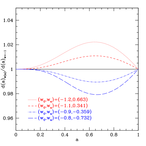
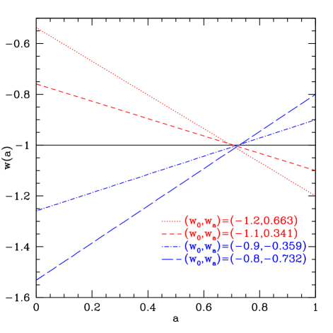
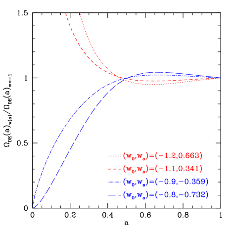
Figure 1 demonstrates an example of how the CMB distance to last scattering forces low redshift experiments to measure $w=-1$. While the crossover in $w$ between the LCDM fiducial case and the time varying models is not perfect, it is well within the precision of current and imminent experiments. Such experiments insensitive to time variation essentially measure a constant $w$ given by its pivot value, hence $w\approx-1$. The deviations in low redshift distances between the models are less than 2%.

Conversely, note that Eq. (3) implies that to match LCDM for some model with current EOS $w_{0}$ one has $w_{a}=-A(1+w_{0})$. For $|1+w_{0}|<0.2$, the family of models generated in this way will all have the same $d_{\rm lss}$ to within 0.2%, better than the anticipated accuracy of the Planck CMB experiment. Also see Fig. 2 where the matching carries through to $\Omega_{m}(z)$ and the growth of structure.

Figure 1: Matching the distance to CMB last scattering between dark energy models leads to convergence and crossover behaviors in other cosmological quantities. The top panel illustrates the convergence in the distance-redshift relation for models with $w_{0}$ ranging from $-0.8$ to $-1.2$ and corresponding $w_{a}$, relative to the $\Lambda$CDM case. The bottom panel shows how this necessarily leads to a crossover with $w=-1$ at the key redshift for sensitivity of low redshift experiments. The crossover in $w(z)$, and its uniqueness, is impelled by the physics not the functional form. Here we fix $\Omega_{m}$; the text discusses robustness to allowing it to vary.

Figure 2: As Fig. 1, showing how matching $d_{\rm lss}$ leads to convergence and crossover conditions on the dark energy density. This has implications for growth of structure; see francis .

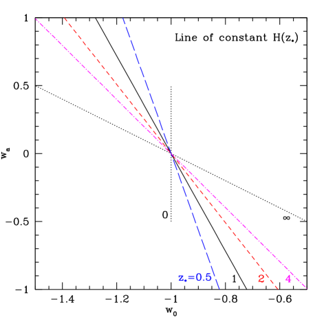
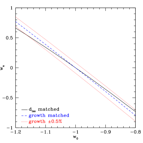
One further implication of the matching-crossover relation for dark energy experiments is that there are unfortunately restrictions to the complementarity between different probes. While techniques may probe the expansion history at various redshifts, hypothetically between $z=0$ and $\infty$, there remain degeneracies despite this range. Measurements of the expansion history (and growth history) depend on the Hubble parameter $H(z)$, or matter density $\Omega_{m}(z)$. Figure 3 shows lines of constant $H(z)$ in the dark energy EOS parameter space. We see that even for measurements at $z=0$ and at $z=\infty$ there is no true orthogonality. This cannot be avoided for techniques involving the Hubble expansion in a simple way (including growth techniques, see coohut ). Theoretically one can achieve full orthogonality, i.e. have a degeneracy direction running between upper right and lower left, by measuring distance ratios (e.g. via strong gravitational lensing linsl ) but this is undone by other degeneracies and systematic uncertainties.

Figure 3: Contours of constant expansion history $H(z)$ span a limited area of the dark energy equation of state plane $w_{0}$-$w_{a}$, even as redshift varies over $z=0-\infty$. Here we hold $\Omega_{m}$ fixed so the lines also represent contours of constant $\Omega_{m}(z)$. Any point along a given $z_{*}$ line represents a dark energy model with the same $H(z_{*})$ as the $\Lambda$CDM model.

Now let us relax the assumptions employed so far. If we consider a family of models with present matter densities different from the fiducial, then the value of $w$ where the models cross upon matching to $d_{\rm lss}$, say, does differ from $-1$. We find that the crossover remains at very close to the previous scale factor $a_{w}=0.7$ but the EOS value at the crossover adjusts to $w_{p}$ given by

$$1+w_{p} = \frac{2}{3(\Omega_{m}^{-1}-1)}\Bigl{[}\int_{1}^{Y}dy\,\{[y^{3}+\Omega_{m}^{-1}-1]^{-1/2}$$ (4)

$$\quad-[y^{3}+\bar{\Omega}_{m}^{-1}-1]^{-1/2}\}\Bigr{]}$$

$$\Big{/}\int_{1}^{Y}dy\,\ln y\,(y^{3}+\Omega_{m}^{-1}-1)^{-3/2},$$

where $\bar{\Omega}_{m}$ is the matter density in the fiducial LCDM model and $\Omega_{m}=\bar{\Omega}_{m}+\Delta\Omega_{m}$ is the model being considered. This formula matches $d_{\rm lss}$ between models with $|\Delta\Omega_{m}|<0.1$ to 0.1%. A good approximation is to take

$$1+w_{p}=3.6\,\Delta\Omega_{m}.$$ (5)

(See also Eq. (2) of fhlt , and note we can apply our formula not just to constant $w$ but to the crossover value of the time varying EOS.)

We can also relax the condition that the CMB measurements tell us precisely the distance to $z=1089$. Planck data (temperature plus polarization) may provide a measurement of the reduced distance to last scattering of 0.4%. Allowing for errors in $d_{\rm lss}$, so models need not exactly match the LCDM fiducial best fit, introduces a scatter of

$$\sigma(w_{p})\approx(+0.01,-0.02)\,\frac{|1+w_{0}|}{0.1}\,\frac{\delta d/d}{0.4\%}\,.$$ (6)

The pivot scale factor stays near $a=0.7$.

Thus, generalization of the CMB constraints to allow for uncertainty in the matter density and the last scattering distance measurement still preserves the implication that (so long as CMB data are consistent with a cosmological constant and – a crucial point – the uncertainty in the matter density is not too great) low redshift data will be driven to show $w\approx-1$. Despite this apparent confirmation of a cosmological constant, the dark energy models considered in Fig. 1 actually have substantial true time variation, up to $|w_{a}|\approx 1$. Therefore measurements of $w=-1\pm 0.05$, say, by ongoing and near term experiments do not provide real support for a cosmological constant. Within the dark energy picture presented here, almost no answer other than $w=-1$ could have been expected. Only future measurements directly sensitive to time variation can truly add to knowledge of whether $w=-1$ or not.

III Robust Parametrization

One possible loophole in the picture presented is if the dark energy behavior differs substantially from the parametrization for $w(z)$ we adopted. However we emphasize that the form $w(z)=w_{0}+w_{a}z/(1+z)$ does not force models to cross and certainly does not force them all to cross at the same scale factor. They are impelled to do so by the physics not the form. Nevertheless, we want to ensure that this parametrization is a robust description of a wide range of dark energy behaviors, especially at high redshift. This has been addressed in a number of articles, e.g. linprl ; linbias , but here we concentrate on testing high redshift and deviations from a linear dependence on scale factor $a$.

One model specifically designed to consider dark energy influence at high redshift is the bending model of wett , with

$$w(z)=w_{0}\,[1+b\ln(1+z)]^{-2}.$$ (7)

The bending parameter $b$ is directly related to the early dark energy density $\Omega_{e}=\Omega_{w}(z\gg 1)$. We consider $w_{0}=-0.9$ and $b=0.415$, corresponding to $\Omega_{e}=0.02$, close to the maximum allowed by data. Note that in contrast $\Omega_{\Lambda}(z=1089)\approx 10^{-9}$. While the $w_{0}$-$w_{a}$ model was not designed to fit early dark energy, it does an admirable job. The model $(w_{0},w_{a})=(-0.9,0.7)$ can match SN distances in the bending model to better than 0.004 magnitudes out to $z=2$ and agrees on $w(z)$ out to $z=2$ to 2%, while $d_{\rm lss}$ is within 0.4%.

Suppose we want to investigate dark energy with a more rapid evolution than apparent from the $w_{a}$ model, and are willing to include a third parameter. Consider model 3.1 of lh05 ,

$$w(a)=w_{0}+w_{a}(1-a^{b}),$$ (8)

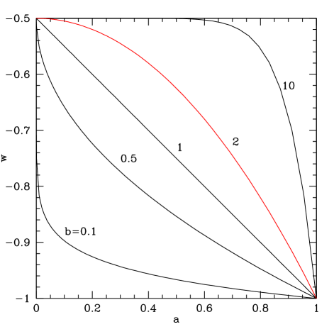
where the usual $w_{a}$ model corresponds to $b=1$. Figure 4 shows the diverse time variation as we adjust $b$. Despite this, the standard $w_{a}$ model can successfully fit variations that are not too extreme, $b\lesssim 2$, to good accuracy. Taking a fairly substantial time evolution, from $w_{0}=-1$ to $w(z\gg 1)=-0.5$, we find that the pure $w_{a}$ model fits $w(z)$ to 0.6%, 1.6% (2%, 4.5%) accuracy compared to the cases with $b=0.5$, 1.5 at $z=0.5$ ($z=2$), and SN distances to 0.005 mag out to $z=2$ and $d_{\rm lss}$ to 0.07%. Only very rapid variations, with $b>2$, corresponding to $dw/dz>1$ today, will cause problems for the standard $w_{a}$ parametrization.

Figure 4: Equation of state as a function of scale factor for the form $w(a)=w_{0}+w_{a}(1-a^{b})$, with curves labeled by $b$. Increasing $b$ gives more rapid time variation recently. The standard $w_{0}$-$w_{a}$ form provides a robust fit for equation of state and distances for all cases $b\lesssim 2$, corresponding to $w_{a}\lesssim 1$.

One could also alter the time characterizing when the EOS variation occurs, with a third parameter as in the extension model of rapaw ,

$$w(z)=\frac{w_{\infty}z+w_{0}z_{t}}{z+z_{t}},$$ (9)

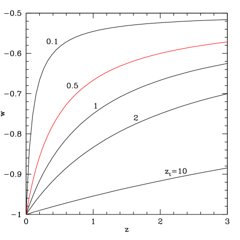
where $w_{\infty}=w(z\gg 1)$ and this form reduces to the $w_{a}$ model for a transition redshift $z_{t}=1$. The impact of such variation on the EOS is shown in Fig. 5, with smaller $z_{t}$ causing a more rapid transition in the recent universe. Again, the usual $w_{a}$ model can encompass this behavior, reproducing $w(z)$ even in the substantially time varying case of $w_{0}=-1$, $w_{\infty}=-0.5$ to within 1%, 4% (4%, 8%) for $z_{t}=2$, 0.5 at $z=0.5$ ($z=2$). Distances agree to within 0.013 mag out to $z=2$ and to 0.002% for $d_{\rm lss}$. Only very rapid variations, with $z_{t}<0.5$, corresponding to $dw/dz>1$ today, will cause problems for the standard $w_{a}$ parametrization.

Figure 5: Equation of state as a function of redshift for the form $w(z)=(w_{\infty}z+w_{0}z_{t})/(z+z_{t})$, with curves labeled by $z_{t}$. Decreasing $z_{t}$ gives more rapid time variation recently. The standard $w_{0}$-$w_{a}$ form provides a robust fit for equation of state and distances for all cases $z_{t}\gtrsim 0.5$, corresponding to $w_{a}\lesssim 1$.

Note that in none of the three forms we have considered have we applied an optimization for the $w_{a}$ fit utilizing the distance matching-crossover physics discussed in §II, i.e. we have not deliberately matched distances. These cases demonstrate that the standard $w_{0}$-$w_{a}$ parametrization has substantial robustness, even for fairly rapidly varying EOS behavior or dark energy with significant presence at high redshifts. The $w_{a}$ robustness is not perfect, of course; very rapid variation, with $w_{a}>1$, or significant nonmonotonic behavior in $w(z)$ will cause the parametrization to break down. However, for a large variety of behavior, and in particular behavior where an averaged EOS $w$ might be thought to hold insight, the $w_{a}$ parametrization is robust and the conclusions of §II regarding the appearance of $w=-1$ are not in jeopardy.

It is interesting to go one step further, and consider the growth history as an observable. Recall that linwhite ; francis showed there exists (within general relativity) a close relation between the distance to CMB last scattering and the linear growth factor of density perturbations. We illustrate this relation in Fig. 6 for the ratio of growth factors $g(a=0.35)/g(a=1)$ identified in linwhite . We can also ask what a measurement of the absolute linear growth factor at, say, $z=2$ can teach us about the high redshift dark energy behavior. Fixing the characteristics of the low redshift universe, say $\Omega_{m}=0.28$ and $w_{0}=-1$, if the growth at $z=2$ agrees with the LCDM model to 5% then within the $w_{a}$ model (which, recall, works well for early dark energy) we can limit $w_{a}<0.6$ or $w(z=2)<-0.6$.

Figure 6: Matching the CMB distance to last scattering is closely related to matching the particular linear growth factor ratio $g(a=0.35)/g(a=1)$ of linwhite . Here we show the similarity of degeneracy directions in the dark energy equation of state plane, with $\Omega_{m}=0.234$.

IV Problems in Parametrization

Despite the success of the $w_{0}$-$w_{a}$ model, one might be tempted to extend it to more parameters, such as the three parameter models discussed in §III, or more general high order polynomial fits. However, the number of EOS parameters that can be accurately fit by even the combination of next generation data has been shown to be limited to two lh05 . Nevertheless, let us explore this slightly further.

One might wish to consider more parameters and simply marginalize over the extra parameters beyond two. If this works, i.e. does not strongly degrade the main two parameters’ estimation, then this effectively allows more freedom in the functional form.

Consider the “ab” form of Eq. (8). Next generation SN+CMB data cannot fit the third parameter and including $b$ weakens estimation of $w_{0}$ and $w_{a}$ by more than an order of magnitude. Further addition of next generation weak lensing data does not help. However, we find that if we place a prior on the third parameter, then while the third parameter is not better determined than our input prior, the first two EOS parameters are not strongly degraded when the prior satisfies

$$\sigma_{b}<\frac{1}{3\sim 10}\frac{1}{w_{a}}.$$ (10)

For the coefficient $1/3$ ($1/10$), the degradation in $w_{a}$ is 15-20% ($\sim$2%), in $w_{0}$ is less than 1%, and in the always more unstable pivot value $w_{p}$ is 60-130% (10-30%). When $w_{a}<0$ then the required prior is weaker, with the $1/3$ coefficient acting as strongly as the $1/10$ coefficient does for positive $w_{a}$.

The main effect of a constrained third, marginalized parameter is therefore a thickening of the confidence contour (greater covariance) rather than an elongation of the confidence interval of the parameter values. In this sense, it acts substantially like a systematic uncertainty, but here the prior or limit on the uncertainty, e.g. $\sigma_{b}$, is likely arbitrary. So exploration of a third parameter can enlarge the freedom of the functional form of $w(z)$, but within arbitrary limits. It also weakens the main parameter estimation. That penalty will be most severe when considering “figures of merit” based on the area $\sigma(w_{p})\cdot\sigma(w_{a})$ of the confidence region, but relatively benign if the main physical questions involve $\sigma(w_{0})$ or $\sigma(w_{a})$ as discussed by linbias .

To check these results, we also considered the $w_{\rm ext}$ form of Eq. (9). This leads to very similar conclusions, that to avoid degradation of the main two EOS parameters one needs a prior on the third parameter $z_{t}$ of order

$$\sigma_{z_{t}}<\frac{1}{3w_{a}},$$ (11)

where $w_{a}=w_{\infty}-w_{0}$. Note that rapaw considered marginalization over $z_{t}$ with a prior of 0.5 and $w_{a}\approx 0.6$. In both the ab and ext cases one can understand the required magnitude of the prior, Eqs. (10)-(11), by studying the form of the Hubble parameter.

While these instances of adding EOS parameters beyond two are fairly benign under the given conditions, using many parameter forms can be not only useless (since only two parameters can be fruitfully constrained) but dangerous. For example, consider a general fourth order polynomial

$$w(z)=w_{0}+\sum_{i=1}^{4}w_{i}\,[\ln(1+z)]^{i},$$ (12)

as discussed in riess06 . Attempting to fit five EOS parameters does not yield useful information even with the combination of next generation data, as mentioned above. However, its implementation does create pathologies, biasing the results.

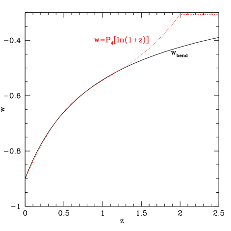
Consider the bending case of Eq. (7) that is adept at describing early dark energy. We saw that the $w_{a}$ parametrization could match this to high accuracy. However, the polynomial form of Eq. (12) is unbounded at high redshift and so must be cut off. In riess06 and in its use for projection of a next generation dark energy mission, the convention is to fix $w=-1$ for $z>2$. Let us examine the consequences of this.

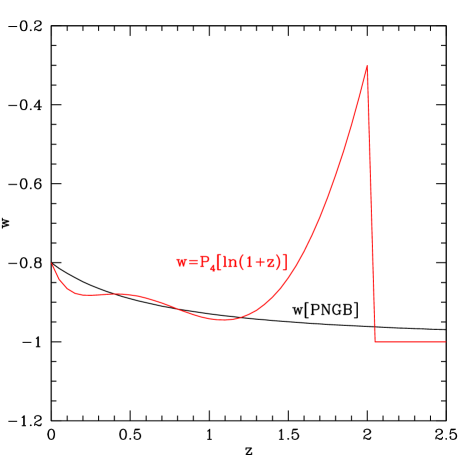
Suppose we could tune the fourth order polynomial to match exactly at $z\leq 2$ the EOS in the bending case of $w_{0}=-0.9$, $b=0.415$ considered in §III. Then due to the cutoff it will misestimate the distance to CMB last scattering by 2.2%, greater than not only Planck precision but current WMAP precision. Instead let us adjust the polynomial coefficients to match $d_{\rm lss}$ and $w(z)$ at $z=0$, 0.4, 0.8, and 1.2. One might think that this would provide excellent approximation to the EOS and the distances – after all, one is matching many more quantities than the mere two of $w_{0}$, $w_{a}$. However, the result, shown in Fig. 7, is that the fourth order polynomial wildly oscillates. This form misestimates SN distances by 0.075 mag (recall that $w_{a}$ succeeded to within 0.004 mag, almost 20 times better).

Figure 7: The fourth order polynomial form (12) for $w(z)$ exhibits pathological behavior and poor fit to equation of state and distances even when fixed to the true $w(z)$ at four redshifts and matched to give the correct $d_{\rm lss}$. Here the true model is the bending form (7) for early dark energy.

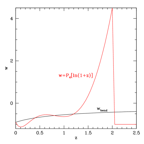
This pathology can be traced to the cutoff at $z>2$. As with spline fits, the freedom in the form often leads to spurious wiggles, especially if the boundary conditions are not carefully chosen. Even thawing dark energy models, which indeed approach $w(z\gg 1)=-1$, are not well fit by the fourth order polynomial form. Taking a simple PNGB dark energy model $w(z)=-1+(1+w_{0})(1+z)^{-F}$ with $w_{0}=-0.8$ and $F=1.5$ yields the results in Fig. 8. In fact, in seeking a nonpathological fit one is driven to $w_{2}=w_{3}=w_{4}=0$, back to a two parameter form such as $w_{0}$, $w_{a}$ so successfully demonstrates.

Figure 8: As Fig. 7, but for the PNGB thawing dark energy model, showing that the pathology in the fourth order polynomial persists even for models that approach $w=-1$ at high redshift.

One can ameliorate considerably the problems of the fourth order polynomial by instead choosing $w(z>2)=w(z=2)$, or more generally

$$w(z>z_{\rm cut})=w(z=z_{\rm cut}).$$ (13)

This delivers much better results: the distances out to $z=2$ in the bending case are now within 0.002 mag of the true values (also see Fig. 9). However, this merely fixed a problem that should never have arisen: the data can actually fit no more than two EOS parameters so there is no point in considering high order polynomials.

Figure 9: As Fig. 7, but we remove the condition $w(z>2)=-1$ and instead use $w(z>2)=w(z=2)$. This tames the spurious oscillations considerably. However, note that the form (12) using five parameters still has difficulties fitting a two parameter equation of state model.

V Conclusion

Given accurate measurement of the distance to CMB last scattering consistent with LCDM, interpreting low redshift distance data leading to $w=-1$ as evidence for a cosmological constant considerably overstates the case. By the nature of $z\lesssim 1.5$ observations with insufficient accuracy to recognize time variation in the equation of state, they essentially measure an averaged $w$ or equivalent constant $w$ just where the CMB data and the cosmological relation between distance and EOS ineluctably predict that constant $w=-1$ to a few percent accuracy.

Even models with time variation $w_{a}\approx 1$ can appear to show $w=-1$ when viewed by these experiments. Such measurements of $w\approx-1$ induce a false sense of security in $\Lambda$. To achieve true insight into the nature of dark energy, even as to simply whether or not it is a cosmological constant, requires measurements capable of directly probing the time variation with significant sensitivity. Current and near term experiments serve a valuable and necessary role in developing techniques and tightening controls on systematic uncertainties.

These conclusions arise within a parametrization of the dark energy behavior, at least over the range where it significantly affects the distance-redshift relation, of $w(z)=w_{0}+w_{a}z/(1+z)$. Checking this assumption, we find this form provides an excellent, robust approximation to a wide variety of behaviors, even fairly rapidly evolving ones $w_{a}\lesssim 1$ (though we have not considered nonmonotonic behaviors, which are not expected from single field models traced over the age of the universe, and as seen can easily be spurious, from noise or improper fits).

Apart from the issue of $w=-1$, attempting to fit the equation of state with more than two parameters is not only fruitless (if significant accuracy is desired) but can lead to pathologies. We have demonstrated this in the case of a proposed fourth order polynomial. One can also attempt to marginalize over a third parameter, to expand the functional freedom, but it is unclear what this gains (since $w_{0}$-$w_{a}$ does a good job fitting these forms on its own) and it requires an arbitrary prior on the third parameter to prevent bloating of the confidence regions of the other parameters.

Even for the basic question of whether the dark energy is Einstein’s cosmological constant, there do not appear to be any short cuts before a carefully designed experiment to constrain accurately the time evolution of the dark energy equation of state, $w(z)$ not merely $w$.