Abstract

We report on a calculation of the effects of supersymmetry on the cross-section for $t-\bar{t}$ production at LHC. A numerical study is carried out for the ten benchmarks of the Snowmass accord. It is found that the higher order effects involving supersymmetric particles in internal loops can be as high as 6%, both for the cross-section and the (parity even) helicity asymmetry, for one particular benchmark. For other benchmarks smaller but nonetheless observable corrections are found.

Keywords: Hadron Colliders, Supersymmetry, Higher-order calculations.

1 Introduction

For nearly 35 years, supersymmetry (SUSY) has been an attractive theory in particle physics. At the most theoretical level, it permits the construction of string theories which do not contain tachyonic states, and at the phenomenological level it offers an explanation for the naturalness of the hierarchy through its reduced ultraviolet divergences, as well as providing resolutions of several puzzles arising in standard models of cosmology. It also gives rise to a correction to the running of the couplings, so that the strong, weak, and electromagnetic interactions can unify at some Grand Unified (GUT) scale.

However, to date there has been no reliable evidence that this theory describes Nature, so that if SUSY is indeed realised in nature, it must be broken at a scale higher than that reached in accelerator experiments conducted up to now. If the theory is to be effective in providing a solution to the naturalness of the hierarchy problem, then the supersymmetry breaking scale cannot be much more than about 1 TeV. This is also the scale of SUSY breaking which leads to unification of couplings. This implies that, with the exception of some hidden corners of parameter space, SUSY is expected to be discovered at the forthcoming LHC.

Clearly the most dramatic manifestation of SUSY would be the production and identification of supersymmetric partner particles such as the spin-$\frac{1}{2}$ charginos or neutralinos, or evidence that at sufficiently high energies hadrons display behaviour consistent with the existence of squarks or gluinos in the sea. Nevertheless, the existence of supersymmetry will have indirect but measurable effects on the cross-sections for the production of Standard Model (SM) particles. The LHC is expected to achieve sufficient integrated luminosity such that it will be possible to determine these cross-sections with sufficient accuracy to be able to detect the effects of higher order corrections coming from loops of supersymmetric particles. The loops can give rise to a significant correction to the production cross-sections even below the threshold for the production of the supersymmetry particles themselves, so that hints that some new physics is imminent can be deduced before the threshold energies are actually reached. Above these thresholds, differential cross-sections with respect to suitably chosen variables can display structures which can be used to determine masses of some of the scalar particles of the MSSM.

In this paper, we consider the influence of the minimal supersymmetric extension of the Standard Model (MSSM) to the production of top-antitop $t-\bar{t}$. At LHC, after an integrated luminosity of 100 $\mathrm{fb^{-1}}$, one expects around $2\times 10^{7}$ such events, so that small corrections should be easily identifiable, not only at the level of the total production cross-section, but also for differential cross-sections with respect to the transverse momentum, $p_{T}$ of the $t$-quark, and also with respect to the invariant mass $M_{t\bar{t}}$, of the $t-\bar{t}$ pair. Both of these are expected to be measured accurately at LHC. The latter variable is one for which differential cross-sections display a discernible structure as one crosses various thresholds. Apart from statistical errors, there will be larger systematic errors arising form uncertainties in the incident beam flux and in the parton distribution functions (PDF’s). Such systematic errors are cancelled in the ratio of helicity asymmetries to total cross-section, defined in Eqs.(15) and (16). Although the helicities of individual $t$- or $\bar{t}$-quarks cannot be determined on an event-by-event basis, their distributions can be inferred from the angular distributions of the decay products (see [1]). The corrections to these asymmetries can be as high as 5 %.

Although the MSSM has very few extra parameters in the supersymmetry conserving sector, the supersymmeric breaking terms can introduce 105 parameters in addition to the 19 parameters of the SM. Clearly, it is impossible to analyse the complete space of these parameters. Nevertheless, we have therefore organised our calculation so that software is available to calculate differential cross-sections with all possible helicity configurations and any given set of SUSY parameters. We have done this by working in terms of helicity matrix-elements and setting up “prototype graphs” which can then be included in the calculation with any combination of couplings and internal masses. This provides maximum flexibility for the extraction of total or differential cross-sections, helicity asymmetries, etc. as well adaptability to other SUSY models. The library was also designed to scan efficiently over a large number of parameter sets. This was achieved by keeping, for one set of kinematic parameters, a table of all required Veltman-Passarino functions in memory, thus avoiding to re-calculate these functions for each new set of model parameters. This can reduce the computation time by up to 60% and makes scans over one or even two-dimensional parameter spaces feasible.

The number of independent SUSY parameters is greatly reduced if one considers supersymmetry scenarios which are consistent with super-gravity or in which SUSY breaking is either gauge-mediated or mediated by the Weyl anomaly. At the Snowmass meeting of 2002, [5], a collection of ten typical models was considered and sets of SUSY parameters for these models were generated. For convenience, we have investigated the effects of SUSY corrections to $t-\bar{t}$ production for these ten parameter sets. We find considerable variation in the magnitudes of the corrections from these different parameter sets. Conversely, this means that accurate measurement of the $t-\bar{t}$ production cross-section can be used as a tool to help identify the correct set of SUSY parameters.

At sufficiently high (partonic) energies, the SUSY corrections to $t-\bar{t}$ production are expected to be dominated by single and double logarithms of incoming parton energy divided by the SUSY breaking scale, $M_{SUSY}$. The determination of these logarithms is independent of the SUSY parameter set, with the exception of $M_{SUSY}$ and the ratio, $\tan\beta$, of the vacuum expectation values of the two Higgs doublets, and the calculation is simplified by the fact that the mixing of various supersymmetric particles to form mass eigenstates has no effect on these logarithms. The logarithmic contributions have been calculated by Beccaria et. al. [9]. One may have expected that it would have been possible to express the entire SUSY correction in terms of these logarithms plus a constant off-set, which depended on the SUSY parameter set. We have compared our results with those of ref.[9] and although it is indeed the case that our results agree with these logarithms plus a constant off-set at sufficiently high partonic energies, this approximation is found to be unsuitable at typical partonic energies which will be reached at LHC, and the entire calculation is required for a reliable prediction of the cross-sections at LHC.

The structure of this paper is as follows: In section 2 we discuss the general method for the extraction of the above-mentioned helicity matrix-elements at the partonic level from a general Feynman graph. In section 3 we list all the prototype graphs and indicate which supersymmetric particles can contribute for each of the prototypes. In section 4 we discuss the results after folding the partonic cross-sections with PDF’s and show the results for the ten Snowmass benchmark points. Section 5 presents some conclusions.

2 Helicity Matrix Elements

Because we wish to be able to discuss the total and differential cross-sections for given helicities of the $t$- and $\bar{t}$- quarks as well as the asymmetries, we find it convenient to work at the parton level for a generic process

$$p_{a}(\lambda_{a})\,+\,p_{b}(\lambda_{b})\ \to\ p_{1}(\lambda_{1})\,+\,p_{2}(\lambda_{2})$$

in terms of helicity matrix-elements ${\cal A}_{\lambda_{a},\lambda_{b},\lambda_{1},\lambda_{2}}(E,\theta)$, as functions of the partonic centre-of-mass energy, $E$ and scattering angle $\theta$ (also in the centre-of-mass).

In the case of quark-antiquark annihilation, for which we take the incoming quarks and antiquarks to be massless, the helicities of the incoming partons are anti-correlated ($\lambda_{a}=-\lambda_{b}$), and although it is possible for this initial helicity anti-correlation to be violated at the one-loop level, the interferences at ${\cal O}(\alpha_{s}^{3})$ or ${\cal O}(\alpha_{s}^{2}\alpha_{W})$ always respect this anti-correlation. On the other hand, for the gluon fusion process there need be no correlation between gluon helicities.

Once these helicity matrices have been determined, differential cross-sections and asymmetries can be computed by convolution with the corresponding parton distribution functions (PDF), summed over helicities or not, as appropriate.

A further potential advantage of the helicity matrix-element formalism, although not currently applicable at LHC, is the determination of initial beam polarisation asymmetries, should it become possible in the future to polarise these beams. For interactions of a parity violating nature such as SUSY corrections to weak interactions, such asymmetries would be immensely useful in identifying the parameters of the supersymmtery model.

The helicity amplitudes are obtained in two stages. In the first stage, a set of coefficient functions, $a^{\{\ \alpha\}}_{\lambda_{a},\lambda_{b}}(E,\theta)$, of complete set of Dirac $\gamma$-matrices, is determined:

$${\cal A}_{\lambda_{a},\lambda_{b},\lambda_{1},\lambda_{2}}(E,\theta)\ =\ \sum_{\{\alpha\}}a^{\{\alpha\}}_{\lambda_{a},\lambda_{b}}(E,\theta)\bar{u}(p_{1},\lambda_{1})\Gamma^{\{\alpha\}}v(p_{2},-\lambda_{2})$$ (1)

where $\Gamma^{\{\alpha\}}$ are the matrices

$$\Gamma_{V}^{\mu} = \gamma^{\mu}$$

$$\Gamma_{A}^{\mu} = \gamma^{\mu}\gamma^{5}$$

$$\Gamma_{T}^{\mu\nu} = \sigma^{\mu\nu}$$ (2)

with associated projection operators $P^{\{\alpha\}}$

$$P_{V}^{\mu} = \frac{1}{4}\left(\gamma^{\mu}+\frac{p_{1}^{\mu}}{m_{t}}\right)$$

$$P_{A}^{\mu} = \frac{1}{4}\left(\gamma^{5}\gamma^{\mu}+\gamma^{5}\frac{p_{1}^{\mu}}{m_{t}}\right)$$

$$P_{T}^{\mu\nu} = \frac{1}{8}\sigma^{\mu\nu}$$ (3)

, such that

$$\mathrm{Tr}\left(\Gamma^{\{\alpha\}}P_{\{\beta\}}\right)\ =\ \delta^{\{\alpha\}}_{\{\beta\}}.$$

Note that the coefficient functions are independent of the helicities of the $t$- and $\bar{t}$ quarks

For the basis vectors $e_{0}\cdots e_{3}$, where

$$e_{0}^{\mu} = \frac{1}{2E}\left(p_{1}^{\mu}+p_{2}^{\mu}\right)$$

$$e_{1}^{\mu} = \frac{1}{2Ep\sin\theta}\left(-(p+E\cos\theta)p_{1}^{\mu}+(p-E\cos\theta)p_{2}^{\mu}+2p\,p_{a}^{\mu}\right)$$

$$e_{2}^{\mu} = \frac{1}{2E^{2}p\sin\theta}\epsilon^{\mu}_{\nu\rho\sigma}p_{1}^{\nu}p_{2}^{\rho}p_{a}^{\sigma}$$

$$e_{3}^{\mu} = \frac{1}{2p}\left(p_{1}^{\mu}-p_{2}^{\mu}\right)$$

($p$ being the magnitude of the three-momentum of the $t$-quark in the centre-of-mass frame), the helicity matrix elements are given by

$${\cal A} = 2\left[E\left(-a_{V}^{1}+i\lambda_{1}a_{V}^{2}\right)+ip\left(a_{A}^{2}+i\lambda_{1}a_{A}^{1}\right)-im_{t}\left(a_{T}^{01}-i\lambda_{1}a_{T}^{02}\right)\right]\delta_{\lambda_{1},-\lambda_{2}}$$ (4)

$$+ 2\left[m_{t}\,a_{A}^{0}-p\,a_{T}^{12}-i\,E\,\lambda_{1}a_{T}^{03}-m_{t}\,\lambda_{1}a_{V}^{3}\right]\delta_{\lambda_{1},\lambda_{2}}$$

Figure 1: Tree-level graph for $t-\bar{t}$ production from quark-antiquark annihilation.

Thus, for example, the non-zero coefficient functions for the quark-antiquark annihilation process at the tree-level (Figure 1) are:

$$a_{V}^{1} = g_{s}^{2}\frac{\cos\theta}{2E}\delta_{\lambda_{a},-\lambda_{b}}\left({\mbox{\boldmath$\tau$}}\otimes{\mbox{\boldmath$\tau$}}\right)$$

$$a_{V}^{2} = g_{s}^{2}\frac{i\lambda_{a}}{2E}\delta_{\lambda_{a},-\lambda_{b}}\left({\mbox{\boldmath$\tau$}}\otimes{\mbox{\boldmath$\tau$}}\right)$$

$$a_{V}^{1} = g_{s}^{2}\frac{\sin\theta}{2E}\delta_{\lambda_{a},-\lambda_{b}}\left({\mbox{\boldmath$\tau$}}\otimes{\mbox{\boldmath$\tau$}}\right),$$ (5)

where $\left({\mbox{\boldmath$\tau$}}\otimes{\mbox{\boldmath$\tau$}}\right)$ indicates the colour factor for a single gluon exchange. Inserting these expressions for the coefficents into eq.(4) generates the helicity matrix-element

$${\cal A}_{\lambda_{a},\lambda_{b},\lambda_{1},\lambda_{2}}(E,\theta) = -g_{s}^{2}\left(\lambda_{a}+\cos\theta\right)\delta_{\lambda_{a},-\lambda_{b}}\delta_{\lambda_{1},-\lambda_{2}}\left({\mbox{\boldmath$\tau$}}\otimes{\mbox{\boldmath$\tau$}}\right)$$ (6)

$$-g_{s}^{2}\frac{m_{t}}{E}\lambda_{1}\sin\theta\,\delta_{\lambda_{a},-\lambda_{b}}\delta_{\lambda_{1},\lambda_{2}}\left({\mbox{\boldmath$\tau$}}\otimes{\mbox{\boldmath$\tau$}}\right),$$

$$\mathalign{\raisebox{-26.40314pt}{\includegraphics{hel-tree_s}}}+\mathalign{\raisebox{-26.7667pt}{\includegraphics{hel-tree_t}}}+\mathalign{\raisebox{-26.40314pt}{\includegraphics{hel-tree_u}}}$$

Figure 2: Tree-level graphs for $t-\bar{t}$ production from gluon fusion.

whereas for the gluon fusion process (Figure 2), the non-zero coefficients are given by

$$a_{V}^{1} = \frac{g_{s}^{2}}{2E(E-p\cos\theta)}\tau^{b}\tau^{a}\left\{E\sin\theta\left(\cos\theta-2\right)\delta_{\lambda_{a},\lambda_{b}}+2p\sin\theta\cos\theta\right\}$$

$$\ \ \ +\left[\tau^{a}\leftrightarrow\tau^{b},\ \lambda_{a}\leftrightarrow\lambda_{b},\ \theta\to(\pi+\theta)\right]$$

$$a_{V}^{2} = \frac{ig_{s}^{2}}{2E(E-p\cos\theta)}\tau^{b}\tau^{a}p\,\sin\theta\,\lambda_{a}\delta_{\lambda_{a},-\lambda_{b}}\ \ \ +\left[\tau^{a}\leftrightarrow\tau^{b},\ \lambda_{a}\leftrightarrow\lambda_{b},\ \theta\to(\pi+\theta)\right]$$

$$a_{V}^{3} = \frac{g_{s}^{2}}{2E(E-p\cos\theta)}\tau^{b}\tau^{a}\left\{-E\cos\theta\left(\cos\theta-2\right)\delta_{\lambda_{a},\lambda_{b}}+2p\sin^{2}\theta\right\}$$

$$\ \ \ +\left[\tau^{a}\leftrightarrow\tau^{b},\ \lambda_{a}\leftrightarrow\lambda_{b},\ \theta\to(\pi+\theta)\right]$$

$$a_{A}^{0} = \frac{g_{s}^{2}}{2E(E-p\cos\theta)}\tau^{b}\tau^{a}\lambda_{a}\left(p\cos\theta-E\right)\delta_{\lambda_{a},\lambda_{b}}$$

$$\ \ \ +\left[\tau^{a}\leftrightarrow\tau^{b},\ \lambda_{a}\leftrightarrow\lambda_{b},\ \theta\to(\pi+\theta)\right]$$

$$a_{T}^{12} = \frac{g_{s}^{2}}{2E(E-p\cos\theta)}\tau^{b}\tau^{a}m_{t}\cos\theta\delta_{\lambda_{a},\lambda_{b}}\ \ \ +\left[\tau^{a}\leftrightarrow\tau^{b},\ \lambda_{a}\leftrightarrow\lambda_{b},\ \theta\to(\pi+\theta)\right]$$ (7)

leading to a tree-level helicity matrix-element

$${\cal A}_{\lambda_{a},\lambda_{b},\lambda_{1},\lambda_{2}}(E,\theta) = \frac{g_{s}^{2}}{2E(E-p\cos\theta)}\tau^{b}\tau^{a}$$ (8)

$$\times \Bigg{\{}m_{t}\left[2\lambda_{1}\left((E+p)\cos^{2}\theta-2p-4E\cos\theta\right)-2\lambda_{a}E\right]\delta_{\lambda_{1},\lambda_{2}}\delta_{\lambda_{a},\lambda_{b}}$$

$$\left[-2E(E+p)\cos\theta\sin\theta+4E^{2}\sin\theta\right]\delta_{\lambda_{1},-\lambda_{2}}\delta_{\lambda_{a},\lambda_{b}}$$

$$-2\lambda_{1}p\,m_{t}\sin^{2}\theta\delta_{\lambda_{1},\lambda_{2}}\delta_{\lambda_{a},-\lambda_{b}}$$

$$-Ep\sin\theta\left(2\cos\theta+\lambda_{1}\lambda_{a}\right)\delta_{\lambda_{1},-\lambda_{2}}\delta_{\lambda_{a},-\lambda_{b}}\Bigg{\}}$$

$$\ \ \ +\left[\tau^{a}\leftrightarrow\tau^{b},\ \lambda_{a}\leftrightarrow\lambda_{b},\ \theta\to(\pi+\theta)\right]$$

In the case of gluon fusion the contribution from any graph may be written in the form

$$\bar{u}(p_{1},\lambda_{1})\Gamma v(p_{2},-\lambda_{2}),$$

where $\Gamma$ is a sum of strings of $\gamma$-matrices with coefficients that are proportional to couplings, internal and external fermion masses and the Veltman-Passarino (VP) [2] functions arising from the loop integrals. These VP functions have arguments that depend on the internal and external masses as well as on the Mandelstam variables $s,t,u$. The coefficients $a^{\{\alpha\}}$ are simply projected by

$$a^{\{\alpha\}}\ =\ \mathrm{Tr}\left(P^{\{\alpha\}}\Gamma\right).$$ (9)

For the quark-antiquark annihilation process there are two types of contributing graphs:

The first type are graphs for which the fermion lines can be factorised into an initial quark line, $\Gamma^{i}$ and a final $t$-quark line, $\Gamma_{f}$. Again these are sums of string of $\gamma$-matrices with coefficients that are proportional to VP functions. In this case the coefficients $a^{\{\alpha\}}$ are projected by

$$a^{\{\alpha\}}\ =\ \delta_{\lambda_{a},-\lambda_{b}}\mathrm{Tr}\left(\Gamma_{i}\gamma\cdot v\frac{\left(1-\lambda_{a}\gamma^{5}\right)}{2}\right)\mathrm{Tr}\left(P^{\{\alpha\}}\Gamma_{f}\right),$$ (10)

where $v^{\mu}$ is a vector in the plane normal to the incoming momenta $p_{a}$ and $p_{b}$ given by:

$$v^{\mu}\ =\ \frac{1}{\sqrt{2}E\,p\,\sin\theta}\left\{p_{b}\cdot p_{1}p_{a}^{\mu}+p_{a}\cdot p_{1}p_{b}^{\mu}-p_{a}\cdot p_{b}p_{1}^{\mu}+i\lambda_{a}\epsilon^{\mu}_{\nu\rho\sigma}p_{a}^{\nu}p_{b}^{\rho}p_{1}^{\sigma}\right\}$$

Figure 3: Gluino, neutralino, or chargino exchange contribution to $t-\bar{t}$ production from quark-antiquark annihilation

The other type of graph is one in which the fermion lines do not factorise into an initial fermion line and a final-fermion line, but rather into an upper line, $\Gamma_{u}$, and a lower line, $\Gamma_{d}$, in which the incoming quark and outgoing $t$-quarks are connected by the exchange gluino, neutralinos, and charginos,is the $s$-channel. It is graphs of this type that give rise to non-zero amplitudes in the case where the incoming helicities are equal, but such amplitudes do not interfere with the tree-level amplitudes. An example of such a graph is shown in Figure 3.

For such graphs the coefficients $a^{\{\alpha\}}$ are projected by

$$a^{\{\alpha\}}\ =\ \mathrm{Tr}\left(\Gamma_{d}\gamma\cdot v\frac{\left(1-\lambda_{a}\gamma^{5}\right)}{2}\right)\Gamma_{d}P^{\{\alpha\}}$$ (11)

As in the case of most of the contributing graphs, the expressions obtained from Figure 3 for the corrections to the coefficients are too long and unwieldy to be reproduced here

Figure 4: Graph involving the exchange of intermediate Majorana fermions

Finally we note here that in several cases, the internal fermions exchanged in the $s$-channel in such graphs may be neutralinos or gluinos, which are Majorana fermions. In such cases supplementary graphs of the type shown in Figure 4 need to be considered. Great care needs to be taken in handling such graphs. The standard expressions for the propagators of Majorana fermions in which a fermion propagates into a fermion or an ant-fermion propagates into and anti-fermion, are ambiguous up to a sign until the exact ordering of the fermions is determined. In order to ensure that this is effected in a consistent manner it is necessary to determine the fermion ordering of the term in the Wick contraction corresponding to the graph under consideration.

A library has been constructed both in FORTRAN and C++ in which each of the prototype graphs shown in the next section can be determined numerically, as a function of the incoming energy, scattering angle, helicities, couplings and internal masses. We have checked all prototype graphs by selecting different routings of the internal loop momenta and copmparing the results numerically. The numerical values of of the relevant VP functions are determined either using the FF library [3] or LOOPTOOLs [4] These libraries can be found at
http://hep.phys.soton.ac.uk//hepwww/staff/D.Ross/susyttbar/

3 Diagrams

In this section we list the diagrams needed for the computation of SUSY contributions to polarised top-antitop production cross sections. To save space we only draw the different topologies. For further reference, each topology has a label set in typewriter font. An asterisk behind the label indicates that the crossed version of this diagram has to be included as well. A double asterisk indicates that only the crossed version is needed. First or second generation quarks are labelled $q$ and top quarks are labelled $t$. Gluons are denoted as $g$ and always represented by curly lines. Momenta and helicities are given in parentheses behind the label. For example, $t(p,\lambda)$ denotes a top quark with (four-)momentum $p$ and helicity $\lambda$. The generic scalar, vector and fermionic particles in each topology are given uppercase labels $S$, $V$, $F$, etc. For each topology we provide a list of MSSM particles that have to be substituted for the generic ones. For the various MSSM particles we use the notations from [8]. However, unless stated otherwise the generation indices $I$, $J$, etc. only run over the first two generations. The third generation quarks are written explicitly as $t\ (=u^{3})$ and $b\ (=d^{3})$.

3.1 Tree-Level Diagrams

The following prototype diagrams contribute to $t\bar{t}$ production at tree-level:

Dqqbar_sV_tree
$V=\gamma,Z,g$

Dgg_sG_tree

Dgg_tF_tree*

$F=t$

3.2 Self-Energy Diagrams

For our calculation we only need to consider self-energy corrections for fermions and gluons. The SUSY self-energy corrections to fermion propagators only come from scalar particles:

$$\mathalign{\raisebox{-17.3238pt}{\includegraphics{pro-seF-SF}}}$$ (12)

The $s$-channel gluon propagator gets SUSY corrections from fermion and scalar loops:

$$\mathalign{\raisebox{-35.39131pt}{\includegraphics{pro-seG-FF}}}\quad,\quad\mathalign{\raisebox{-35.39131pt}{\includegraphics{pro-seG-SS}}}\quad,\quad\mathalign{\raisebox{-13.21758pt}{\includegraphics{pro-seG-S}}}$$ (13)

The two scalar self-energy diagrams always appear as a pair with the same coefficient and the same scalar particle in the loop. By inserting these self-energy corrections in individual lines of the tree level diagrams we obtain the following self-energy diagrams:

$\mathalign{\raisebox{-69.94331pt}{\includegraphics{pro-qqbar-sG-xseq-1}}}\quad+\quad\mathalign{\raisebox{-70.20097pt}{\includegraphics{pro-qqbar-sG-xseq-2}}}$

Dqqbar_sV_xseSq
$(q,F,S)=(u^{I},\chi^{0}_{j},U_{i}),\ (d^{I},\chi^{0}_{j},D_{i}),\ (u^{I},\chi_{j},D_{i}),\ (d^{I},\chi^{\mathsf{c}}_{j},U_{i}),\ (u^{I},\Lambda,U_{i}),\ (d^{I},\Lambda,D_{i})$

$\mathalign{\raisebox{-69.94331pt}{\includegraphics{pro-qqbar-sG-xset-1}}}\quad+\quad\mathalign{\raisebox{-70.20097pt}{\includegraphics{pro-qqbar-sG-xset-2}}}$

Dqqbar_sV_xseSt
$(F,S)=(\chi^{0}_{j},U_{i}),\ (\chi_{j},D_{i}),\ (t,H^{0}_{i}),\ (t,A^{0}_{1}),\ (b,H_{1}),\ (\Lambda,U_{i})$

Dqqbar_sG_iseF, Dqqbar_sG_iseS
$q=u^{I},d^{I}\quad,\quad F=u^{I},t,d^{I},b,\Lambda\quad,\quad S=U_{i},D_{i}$

$\mathalign{\raisebox{-69.94331pt}{\includegraphics{pro-gg-sG-xseg-1}}}\quad+\quad\mathalign{\raisebox{-71.58113pt}{\includegraphics{pro-gg-sG-xseg-2}}}$

Dgg_sG_xseFg, Dgg_sG_xseSg
$F=\Lambda\quad,\quad S=U_{i},D_{i}$

$\mathalign{\raisebox{-69.94331pt}{\includegraphics{pro-gg-sG-xset-1}}}\quad+\quad\mathalign{\raisebox{-70.20097pt}{\includegraphics{pro-gg-sG-xset-2}}}$

Dgg_sG_xseSt
$(F,S)=(\chi^{0}_{j},U_{i}),\ (\chi_{j},D_{i}),\ (t,H^{0}_{i}),\ (t,A^{0}_{1}),\ (b,H_{1}),\ (\Lambda,U_{i})$

Dgg_sG_iseF, gg_sG_iseS
$F=\Lambda\quad,\quad S=U_{i},D_{i}$

$\mathalign{\raisebox{-80.70149pt}{\includegraphics{pro-gg-tF-xset-1}}}\quad+\quad\mathalign{\raisebox{-90.19255pt}{\includegraphics{pro-gg-tF-xset-2}}}$

Dgg_tF_xseSt*
$(F,S)=(\chi^{0}_{j},U_{i}),\ (\chi_{j},D_{i}),\ (t,H^{0}_{i}),\ (t,A^{0}_{1}),\ (b,H_{1}),\ (\Lambda,U_{i})$

$\mathalign{\raisebox{-80.70149pt}{\includegraphics{pro-gg-tF-xseg-1}}}\quad+\quad\mathalign{\raisebox{-85.39493pt}{\includegraphics{pro-gg-tF-xseg-2}}}$

Dgg_tF_xseSt*
$F=\Lambda\quad,\quad S=U_{i},D_{i}$

Dgg_tF_iseS*
$(F,S)=(\chi^{0}_{j},U_{i}),\ (\chi_{j},D_{i}),\ (t,H^{0}_{i}),\ (t,A^{0}_{1}),\ (b,H_{1}),\ (\Lambda,U_{i})$

In each diagram the hatched blob stands for one of the self-energy corrections from eq:pro:seF or eq:pro:seG.

3.3 Vertex Corrections

The prototype vertex corrections for the $q\bar{q}\to t\bar{t}$ amplitude are:

Dqqbar_sG_vertSq
$(q,F,S)=(u^{I},\Lambda,U_{i}),\ (d^{I},\Lambda,D_{i})$

Dqqbar_sV_vertSt
$q=u^{I},d^{I}$
$(F,S)=(\Lambda,U_{i}),\ (t,H^{0}_{1}),\ (t,A^{0}_{1}),\ (b,H_{1})$

Dqqbar_sG_vertSSq
$(q,F,S)=(u^{I},\Lambda,U_{i}),\ (u^{I},\chi^{0}_{j},U_{i}),\ (u^{I},\chi_{j},D_{i}),$
$(d^{I},\Lambda,D_{i}),\ (d^{I},\chi^{0}_{j},D_{i}),\ (d^{I},\chi_{j},U_{i})$

Dqqbar_sG_vertSSt
$q=u^{I},d^{I}$
$(S,F)=(\Lambda,U_{i}),\ (\chi^{0}_{j},U_{i}),\ (\chi_{j},D_{i})$

For the $gg\to t\bar{t}$ amplitude we distinguish vertex corrections for $s$ and $t$-channel diagrams. The corrections to the $s$-channel diagrams are:

Dgg_sG_vertSt
$(F,S)=(\Lambda,U_{i}),\ (t,H^{0}_{1}),\ (t,A^{0}_{1}),\ (b,H_{1})$

Dgg_sG_vertSSt
$(S,F)=(U_{i},\Lambda),\ (U_{i},\chi^{0}_{j}),\ (D_{i},\chi_{j})$

$\mathalign{\raisebox{-69.94331pt}{\includegraphics{pro-gg-sG-vertFg-ccw}}}\quad-\quad\mathalign{\raisebox{-69.94331pt}{\includegraphics{pro-gg-sG-vertFg-cw}}}$

Dgg_sG_vertFg
$F=\Lambda$

$\mathalign{\raisebox{-69.94331pt}{\includegraphics{pro-gg-sG-vertSg-ccw}}}\quad-\quad\mathalign{\raisebox{-69.94331pt}{\includegraphics{pro-gg-sG-vertSg-cw}}}$

Dgg_sG_vertSg
$S=U_{i},D_{i}$

$\mathalign{\raisebox{-69.94331pt}{\includegraphics{pro-gg-sS-vertFg-ccw}}}\quad+\quad\mathalign{\raisebox{-69.94331pt}{\includegraphics{pro-gg-sS-vertFg-cw}}}$

Dgg_sS_vertFg
$F=t,b\quad,\quad S=H^{0}_{1},A^{0}_{1}$

$\mathalign{\raisebox{-69.94331pt}{\includegraphics{pro-gg-sS-vertSg-ccw}}}\quad+\quad\mathalign{\raisebox{-69.94331pt}{\includegraphics{pro-gg-sS-vertSg-cw}}}$

Dgg_sS_vertSg
$S_{1}=U_{i},D_{i}\quad,\quad S_{2}=H^{0}_{1},A^{0}_{1}$

Dgg_sS_vertSSg
$S_{1}=U_{i},D_{i}\quad,\quad S_{2}=H^{0}_{1},A^{0}_{1}$

The $t$-channel vertex corrections are:

Dgg_tF_vertS1*

$(F,S)=(\Lambda,U_{i}),\ (t,H^{0}_{1}),\ (t,A^{0}_{1}),\ (b,H_{1})$

Dgg_tF_vertS2*

$(F,S)=(\Lambda,U_{i}),\ (t,H^{0}_{1}),\ (t,A^{0}_{1}),\ (b,H_{1})$

Dgg_tF_vertSS1*

$(S,F)=(U_{i},\Lambda),\ (U_{i},\chi^{0}_{j}),\ (D_{i},\chi_{j})$

Dgg_tF_vertSS2*

$(S,F)=(U_{i},\Lambda)$

3.4 Box Diagrams

Dqqbar_boxSS
$(q,S_{1},S_{2},F_{1},F_{2})=(u^{I},U_{i},U_{j},\Lambda,\Lambda),\ (u^{I},U_{i},U_{j},\Lambda,\chi^{0}_{k}),\ (u^{I},U_{i},U_{j},\chi^{0}_{k},\Lambda),$
$(d^{I},D_{i},D_{j},\Lambda,\chi_{k}),\ (d^{I},U_{i},U_{j},\chi_{k},\Lambda)$

Dqqbar_fboxSS
$(q,F_{1},F_{2},S_{1},S_{2})=(u^{I},\Lambda,\Lambda,U_{i},U_{j}),$
$(d^{I},\Lambda,\Lambda,D_{i},U_{j}),\ (u^{I},\chi^{0}_{k},\Lambda,U_{i},U_{j}),$
$(u^{I},\Lambda,\chi^{0}_{k},U_{i},U_{j}),\ (d^{I},\chi^{0}_{k},\Lambda,D_{i},U_{j}),$
$(d^{I},\Lambda,\chi^{0}_{k},D_{i},U_{j})$

Dqqbar_fboxSSx**

$(q,F_{1},F_{2},S_{1},S_{2})=(u^{I},\Lambda,\Lambda,U_{i},U_{j}),$

$(d^{I},\Lambda,\Lambda,D_{i},U_{j}),\ (u^{I},\chi^{0}_{k},\Lambda,U_{i},U_{j}),$

$(u^{I},\Lambda,\chi^{0}_{k},U_{i},U_{j}),\ (d^{I},\chi^{0}_{k},\Lambda,D_{i},U_{j}),$

$(d^{I},\Lambda,\chi^{0}_{k},D_{i},U_{j})$

Dgg_boxFS*

$(F,S)=(\Lambda,U_{i}),\ (t,H^{0}_{1}),\ (t,A^{0}_{1}),\ (b,H_{i})$

Dgg_boxSF*

$(S,F)=(U_{i},\Lambda),\ (U_{i},\chi^{0}_{j}),\ (D_{i},\chi_{j})$

Dgg_boxSFx*
$(S,F)=(U_{i},\Lambda)$

4 Cross Sections and Asymmetries

In this section we present our results for the SUSY corrections to polarised $t\bar{t}$ production cross sections, which we calculated for each of the 10 Snowmass benchmarks detailed in [5]. To calculate the masses of the supersymmetric particles and run the couplings to the TeV scale we used the program SOFTSUSY by B. C. Allanach [6]. The decay widths of the MSSM Higgs particles were calculated with the program HDECAY by Djouadi, Kalinowski and Spira [7]. The Feynman rules for the MSSM vertices were taken from J. Rosiek’s paper [8]. We compare our parton level cross sections with the results obtained in the leading log approximation [9]. Then we discuss our results for the total $pp\to t\bar{t}$ cross section and the double helicity asymmetries introduced in [10].

Let $\hat{\sigma}_{i}$ denote the total cross section for the process $i\to t\bar{t}$, where the initial state $i$ can be a gluon pair ($gg$), a light up-type quark-antiquark pair ($u\bar{u}$) or a light down type quark-antiquark pair ($d\bar{d}$). We regard $\hat{\sigma}_{i}$ as a function of the variable $\hat{s}\equiv M_{t\bar{t}}^{2}$, where $M_{t\bar{t}}$ is the invariant mass of the top-antitop pair. For each of these cross sections we have calculated the leading order contribution $\hat{\sigma}_{i}^{\text{LO}}$ and the SUSY corrections $\hat{\sigma}_{i}^{\text{SUSY}}$ due to the diagrams listed in the previous section. The SUSY corrections can be split into super-QCD (SQCD) corrections and super-electroweak (SEW) corrections. The SQCD corrections are of order $\order(\alpha_{s}^{3})$ and the SEW correction of order $\order(\alpha\alpha_{s}^{2})$. Consequently the SEW corrections are one order of magnitude smaller than the SQCD corrections. We also define the ratios

$$\hat{r}_{i}(\hat{s})=\frac{\hat{\sigma}_{i}^{\text{SUSY}}(\hat{s})}{\hat{\sigma}_{i}^{\text{LO}}(\hat{s})}\eqpunct.$$ (14)

Figures 5, 6 and 7 show a comparison of our “exact” ratios with the results obtained in the leading log approximation by Beccaria, Renard and Verzegnassi [9].

Figure 5: SUSY corrections to the $gg\to t\bar{t}$ cross section in the “exact” calculation and the leading log approximation for benchmark 5 of [5]. The width of the leading log graph reflects the uncertaincy due to the choice of the universal SUSY scale.

Figure 6: SUSY corrections to the $u\bar{u}\to t\bar{t}$ cross section in the “exact” calculation and the leading log approximation for benchmark 5 of [5]. The results for first and second generation up-type quarks are identical. The width of the leading log graph reflects the uncertainty due to the choice of the universal SUSY scale.

Figure 7: SUSY corrections to the $d\bar{d}\to t\bar{t}$ cross section in the “exact” calculation and the leading log approximation for benchmark 5 of [5]. The results for first and second generation down-type quarks are identical. The width of the leading log graph reflects the uncertainty due to the choice of the universal SUSY scale.

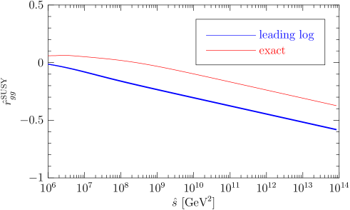
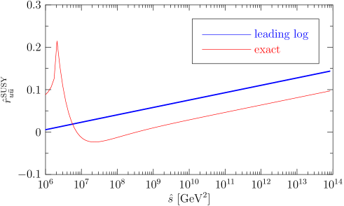
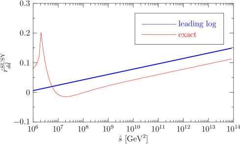
We have used Snowmass benchmark 5 to compute the exact cross section, but the observations stated here are true for any of the 10 Snowmass benchmarks. The only SUSY inputs in the leading log approximation are $\tan\beta$ and a universal SUSY mass scale $M_{\text{SUSY}}$. Sensible values for this scale lie anywhere between the mass of the lightest and the mass of the heaviest SUSY particle. The widths of the leading log graphs in figures 5, 6 and 7 reflect this uncertainly. We see that, in the leading log approximation, the ratios $\hat{r}_{i}^{\text{SUSY}}$ are proportional to $\log(\hat{s}/M_{\text{SUSY}}^{2})$. For $\hat{s}\gtrsim\unit{10^{9}}{GeV}$ the exact ratio runs linear with the same slope, but with a constant offset to the leading log graph. For very large centre of mass energies this offset becomes negligible. Therefore our results agree with the leading log approximation in the high energy limit. However, for collision energies that are achievable at the LHC we see that the leading log approximation fails to reproduce the exact results of the full SUSY calculation, even with the offset included.

To obtain the $pp\to t\bar{t}$ cross sections, the parton level cross sections $\hat{\sigma}_{i}$ were folded with the CTEQ6L1 set of the CTEQ v6.51 parton distribution functions [11]. For the proton-proton collision we assumed a centre of mass energy of 14TeV. Let $d\sigma_{\lambda_{1}\lambda_{2}}/dM_{t\bar{t}}$ denote the invariant mass differential cross section for producing a top quark with helicity $\lambda_{1}$ and an anti-top quark with helicity $\lambda_{2}$. Then we define

$$\frac{d\sigma_{\text{tot}}}{dM_{t\bar{t}}} =\frac{d\sigma_{++}}{dM_{t\bar{t}}}+\frac{d\sigma_{--}}{dM_{t\bar{t}}}+\frac{d\sigma_{+-}}{dM_{t\bar{t}}}+\frac{d\sigma_{-+}}{dM_{t\bar{t}}}\eqpunct,$$ (15a)

$$\frac{d\sigma_{LL}}{dM_{t\bar{t}}} =\frac{d\sigma_{++}}{dM_{t\bar{t}}}+\frac{d\sigma_{--}}{dM_{t\bar{t}}}-\frac{d\sigma_{+-}}{dM_{t\bar{t}}}-\frac{d\sigma_{-+}}{dM_{t\bar{t}}}\eqpunct,$$ (15b)

$$\frac{d\sigma_{PV}}{dM_{t\bar{t}}} =\frac{d\sigma_{+-}}{dM_{t\bar{t}}}-\frac{d\sigma_{-+}}{dM_{t\bar{t}}}\eqpunct.$$ (15c)

For each combination we indicate the leading order and SUSY contributions by superscripts ‘LO’ and ‘SUSY’, respectively. The parity even combinations $d\sigma^{\text{SUSY}}_{\text{tot}}$ and $d\sigma^{\text{SUSY}}_{LL}$ are dominated by the SQCD corrections. However, for the parity odd combination $d\sigma^{\text{SUSY}}_{PV}$ the SQCD corrections are zero, since parity is conserved in super-QCD. For the asymmetries and the SUSY corrections we define the ratios

$$r^{\text{LO}}_{LL/PV}(M_{t\bar{t}})=\frac{d\sigma^{\text{LO}}_{LL/PV}/dM_{t\bar{t}}}{d\sigma^{\text{LO}}_{\text{tot}}/dM_{t\bar{t}}}\qquad,\qquad r^{\text{SUSY}}_{\text{tot}/LL/PV}(M_{t\bar{t}})=\frac{d\sigma^{\text{SUSY}}_{\text{tot}/LL/PV}/dM_{t\bar{t}}}{d\sigma^{\text{LO}}_{\text{tot}}/dM_{t\bar{t}}}\eqpunct.$$ (16)

Figure 8: Leading order results for the invariant mass differential cross section.

Figure 9: Leading order results for the invariant mass $LL$ asymmetry.

Figures 8 and 9 show the results for $d\sigma^{\text{LO}}_{\text{tot}}/dM_{t\bar{t}}$ and $r^{\text{LO}}_{LL}(M_{t\bar{t}})$, respectively. Since there is no parity violation at leading order the ratio $r^{\text{LO}}_{PV}$ is identically zero.

Figures 10 and 11 show the ratios $r^{\text{SUSY}}_{\text{tot}}(M_{t\bar{t}})$ and $r^{\text{SUSY}}_{LL}(M_{t\bar{t}})$ for each of the 10 Snowmass benchmarks.

Figure 10: SUSY corrections to the invariant mass differential cross section for the Snowmass benchmarks. The numbers in the legend refer to the labelling of the benchmarks in [5].

Figure 11: SUSY corrections to the invariant mass $LL$ asymmetry for the Snowmass benchmarks. The numbers in the legend refer to the labelling of the benchmarks in [5].

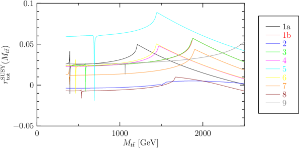
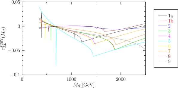
We see that the SUSY corrections to the $t\bar{t}$ cross section can be as large as 10% of the leading order cross section, but typically only reach the 5% level. In both plots we see “resonance peaks” located at the masses of the heavy and the pseudo-scalar Higgs ($H^{0}_{1}$ and $A^{0}_{1}$ in the notation of [8]). They come from the scalar $s$-channel propagators in the diagrams labelled Dgg_sS_vertFg, Dgg_sS_vertSg and Dgg_sS_vertSSg in sectionsec:pro. Note that these particles have negligible coupling to the light quarks extracted from the incoming hadrons, so that they arise from the gluon fusion contribution, in which the exchanged scalars are connected to the incoming gluons via a gluino or squark triangle. Moreover, due to the fermion triangle the sign of the contribution from diagram Dgg_sS_vertFg is opposite that of Dgg_sS_vertSg and Dgg_sS_vertSSg. This explains why we get downward-pointing resonance peaks for some of the benchmarks. Also note that, for all 10 benchmarks, the difference of the heavy and the pseudo-scalar Higgs masses is much smaller than their decay widths. Consequently we can only see two distinct peaks when these peaks have opposite signs. The kinks occurring between 1 and 2TeV coincide, for each benchmark, with twice the gluino mass and can therefore be understood as a threshold effect due to the box diagrams Dqqbar_fboxSS and Dgg_boxFS.

Figurefig:res:pv_mtt shows the SUSY corrections to the parity violating asymmetry for each of the 10 benchmarks.

Figure 12: SUSY corrections to the invariant mass $PV$ asymmetry for the Snowmass benchmarks. The numbers in the legend refer to the labelling of the benchmarks in [5].

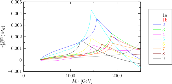
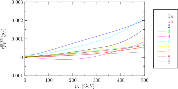
Here the resonance peaks are absent, because the diagrams Dgg_sS_vertFg, Dgg_sS_vertSg and Dgg_sS_vertSSg are parity-conserving. Furthermore, the SUSY corrections to the parity violating asymmetry are one order of magnitude smaller than the corrections to the parity-even observables, because it only gets contributions from interferences of oder $\order(\alpha\alpha_{s}^{2})$.

By integrating the differential cross sections eq:res:asymmetries over $M_{t\bar{t}}$ we obtain cross sections for producing $t\bar{t}$ pairs with arbitrary invariant mass. We define the cross sections $\sigma_{\text{tot}}$, $\sigma_{LL}$ and $\sigma_{PV}$ by

$$\sigma_{\text{tot}/LL/PV}=\int_{2m_{t}}^{M_{pp}}dM_{t\bar{t}}\frac{d\sigma_{\text{tot}/LL/PV}}{dM_{t\bar{t}}}\eqpunct,$$ (17)

where $m_{t}$ is the top mass and $M_{pp}=\unit{14}{TeV}$ is the invariant mass of the proton-proton system. Again, the leading order and SUSY contributions are indicated by superscripts ‘LO’ and ‘SUSY’, respectively. Tabletab:res:cross_sections summarises our results for these cross sections.

hhs[2pt]	σ^LO_tot		σ^SUSY_tot		σ^LO_LL		σ^SUSY_LL		σ^SUSY_PV
h 1a	331.	8	+8.	4	91.	99	+1.	75	+0.	063
1b	288.	3	+6.	9	79.	50	+1.	72	+0.	020
2	266.	3	-1.	0	72.	84	-0.	34	+0.	125
3	289.	5	+6.	9	80.	08	+1.	73	+0.	043
4	307.	6	+7.	1	85.	62	+1.	64	-0.	018
5	332.	1	+19.	8	93.	48	+5.	16	+0.	111
6	310.	8	+7.	4	85.	74	+1.	68	+0.	053
7	284.	9	+3.	5	78.	04	+0.	78	+0.	029
8	271.	2	-1.	9	74.	08	-0.	64	+0.	035
9	263.	6	+6.	9	72.	32	+1.	82	+0.	019
hh

Table 1: Numerical results for the integrated $t\bar{t}$ cross section and asymmetries. The numbers in the left column refer to the labelling of the Snowmass benchmarks in [5]. The superscripts ‘LO’ and ‘SUSY’ indicate leading order results and SUSY corrections, respectively. The cross sections are given in pico-barns (pb).

For both, $\sigma_{\text{tot}}$ and $\sigma_{LL}$ we see that the SUSY corrections typically make up 2% of the leading order results. However, they can be as big as 5% in the case of benchmark 5 and as small as 0.3% in the case of benchmark 2.

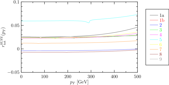
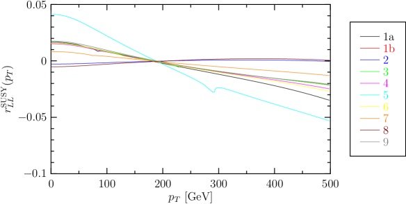
Experimentally it is often more convenient to parametrise the $t\bar{t}$ production cross section by the transverse momentum $p_{T}$ of the top quark. For the transverse momentum differential cross section $d\sigma_{\lambda_{1}\lambda_{2}}/dp_{T}$ we define the total differential cross section $d\sigma_{\text{tot}}/dp_{T}$, the asymmetries $d\sigma_{LL}/dp_{T}$ and $d\sigma_{PV}/dp_{T}$ and the ratios $r^{\text{LO}}_{LL}(p_{T})$, $r^{\text{LO}}_{PV}(p_{T})$, $r^{\text{SUSY}}_{\text{tot}}(p_{T})$, $r^{\text{SUSY}}_{LL}(p_{T})$ and $r^{\text{SUSY}}_{PV}(p_{T})$ in analogy to eq:res:asymmetries and eq:res:ratios. Our results for these quantities are shown in figures 13 to 17. We note here that the “resonance peaks” and “troughs” from the thresholds for scalar particle exchange are smoothed out by the phase-space integration which means that $M_{t\bar{t}}$ is a far better variable in which to analyse the data in order to extract information on the SUSY parameter set, although we note that some of the benchmarks give rise to an enhancement of the differential cross-section of up to 7% at large $p_{T}$.

Figure 13: Leading order results for the transverse momentum differential cross section.

Figure 14: Leading order results for the transverse momentum $LL$ asymmetry.

Figure 15: SUSY corrections to the transverse momentum differential cross section for the Snowmass benchmarks. The numbers in the legend refer to the labelling of the benchmarks in [5].

Figure 16: SUSY corrections to the transverse momentum $LL$ asymmetry for the Snowmass benchmarks. The numbers in the legend refer to the labelling of the benchmarks in [5].

Figure 17: SUSY corrections to the transverse momentum $PV$ asymmetry for the Snowmass benchmarks. The numbers in the legend refer to the labelling of the benchmarks in [5].

5 Conclusions

We have calculated the complete MSSM corrections to the cross-section for $t-\bar{t}$ production at LHC. The calculation has been set up in terms of a set of prototype Feynman graphs for the partonic-level helicity matrix-elements. In this way the prototypes can be used for any set of SUSY parameters by inserting the corresponding couplings and internal masses into the prototypes.

We have obtained numerical results for the ten Snowmass benchmark sets using the CTEQ PDF’s. We find a considerable variation of the effects of the one-loop SUSY corrections between the various benchmarks. The benchmark giving the largest correction is benchmark 5, which is a super-gravity model with small $\tan\beta=5$ and a large negative tri-linear coupling, $A_{0}=-1000$ GeV. These large corrections can be understood from the fact that this large tri-linear coupling generates a light stop mass (258 GeV) thereby enhancing graphs involving a stop mass inside the loop. This gives an enhancement of 6% in the total production cross-section.

Whereas the corrections for the other benchmarks are somewhat smaller, they are usually around 3% and therefroe comaparable to the weak corrections calculated by Bernreuther et. al. [12] and Kuhn et. al. [13]. Note that whereas the weak corrections reported in [12, 13] decrease the prediction for the cross-sections, the SUSY corrections have a positive sign for most of the benchmarks considered.

Statistically, we expect these events to be easily detectable given the anticipated yield of order $10^{7}$ events over the period of running of LHC. We have found similar corrections in the asymmetry ratios defined in in Eqs.(15) and (16). For these asymmetries we also expect cancellation of systematic errors arising from uncertainties in incoming parton fluxes, so that these corrections of order 3% would exceed the statisical errors by a factor of $\sim\,100$.

Given corrections of such significance, it is reasonable to assume that corrections in the differential cross-sections will also be detectable (provided sufficiently large bins are taken). We have therefore plotted the differential cross-sections with respect to the invariant mass $M_{t\bar{t}}$ of the $t-\bar{t}$ system and also with respect to the transverse momentum $p_{T}$ of th $t$-quark. In the former case, the differential cross-sections display an interesting structure with peaks and/or troughs corresponding to thresholds for scalar particle exchanges in the gluon fusion process.

We have also determined the SUSY contribution to the parity odd helicity asymmetry. This receives only contributions from the supersymmetric partners in the weak-interaction sector, which are suppressed relative to the SQCD corrections by ${\cal O}(\alpha_{W}/\alpha_{s})$. It would appear, therefore that even for benchmark 5, which produces the largest corrections, such parity violating asymmetries will be too small to observe.

Acknowledgements:
The authors are grateful to Stefano Moretti and Sacha Belyaev for useful converstaions.

References

- [1] P. Uwer, Phys. Lett. B609 (2005) 271; W. Bernreuther, A. Brandenburg, Z.G. Si and P. Uwer, arXiv:hep-ph/0410197, Nucl. Phys. B690 (2004) 81, Acta Phys. Polon. B 34 (2003) 4477, arXiv:hep-ph/0209202, Int. J. Mod. Phys. A18 (2003) 1357, Phys. Rev. Lett. 87 (2001) 242002, Phys. Lett. B509 (2001) 53; A. Brandenburg, Z.G. Si and P. Uwer, Phys. Lett. B539 (2002) 235; W. Bernreuther, A. Brandenburg and P. Uwer, Phys. Lett. B368 (1996) 153.
- [2] G. Passarino and M. Veltman, Nucl. Phys. B160 (1979) 51
- [3] G.J. van Oldenborgh, Z. Phys C46 (1990) 425
- [4] T. Hahn and M. Perez Victoria Comput. Phys. Commun. 158 (1999) 153
- [5] B. C. Allanach et al., “The snowmass points and slopes: Benchmarks for SUSY searches,” hep-ph/0202233.
- [6] B. C. Allanach, “SOFTSUSY: A C++ program for calculating supersymmetric spectra,” Comput. Phys. Commun. 143 (2002) 305–331, hep-ph/0104145.
- [7] A. Djouadi, J. Kalinowski, and M. Spira, Comput. Phys. Commun. 108 (1998) 56–74, hep-ph/9704448.
-
[8]
J. Rosiek, “Complete set of Feynman rules for the MSSM – ERRATUM,”
hep-ph/9511250.
Update from 17 Sept. 2004,
http://www.fuw.edu.pl/~rosiek. - [9] M. Beccaria, F. M. Renard, and C. Verzegnassi, Phys. Rev. D69 (2004) 113004, hep-ph/0402028.
- [10] C. Bourrely, J. P. Guillet, and J. Soffer, Nucl. Phys. B361 (1991) 72–92.
- [11] J. Pumplin et al., “New generation of parton distributions with uncertainties from global QCD analysis,” JHEP 07 (2002) 012, hep-ph/0201195.
- [12] W. Bernreuther, M. Fücker, and G-Z. Si, Phys. Rev D74 (2006 113005
- [13] J.H. Kuhn, A. Scharf, and P. Uwer, Eur. Phys. J. C51 (2007) 37