Density Matrix Renormalization for model reduction in nonlinear dynamics

Abstract

We present a novel approach for model reduction of nonlinear dynamical systems based on proper orthogonal decomposition (POD). Our method, derived from Density Matrix Renormalization Group (DMRG), provides a significant reduction in computational effort for the calculation of the reduced system, compared to a POD. The efficiency of the algorithm is tested on the one dimensional Burgers equations and a one dimensional equation of the Fisher type as nonlinear model systems.

Nonlinear dynamical systems arise in many fields as physics, e.g. turbulence Sirovich (1987), mathematics and biology Murray (2002). They often require a significant high number of degrees of freedom(dof) for simulation with suitable accuracy. For a large class of systems the solutions are regular, nevertheless the influence of the nonlinearity is essential. Here model reduction (MR) can lead to an efficient description, if the dynamics is effectively confined to a lower dimensional attractor in phase space.

The aim of this work is to develop an algorithm that can find a reduced model for a given system, usually derived from a partial differential equation.

One method to obtain such a reduced description is the so called proper orthogonal decomposition Sirovich (1987); Lucia et al. (2004) (POD). It is obtained by calculating the eigenvectors of the spatial covariance matrix of the field over the phase space, typically by using a empirical spatial covariance matrix from a number of realization of the dynamic evolution. The method itself is linear in that the phase space is reduced to a subspace (in which the relevant Attractor has to be embedded). Nevertheless it accounts for the nonlinearity and gives the ’optimal’ linear reduction possible. By definition the POD requires a simulation of the full, unreduced system and a diagonalization of a symmetric matrix of similar size. While the later can be circumvented by the method of snapshots of Sirovich Sirovich (1987), the simulation in unavoidable.

Within our approach, we try to calculate ’approximate’ POD modes without simulating the full, unreduced system. This is achieved by following concepts from density matrix renormalization. Effectively, we adapt a system of already low dimensionality, to reproduce the full dynamics optimally. Consequently, all calculations are performed on low dimensional systems. In exchange several calculation steps have to be performed, but their number is proportional to the size of the full system of interest. Practically this is one possible way to study large dynamical systems, although within this work we are still restricted to spatially one dimensional systems. Beside from possible benefits for the efficiency, an interesting question is whether it is possible to reconstruct dynamic behavior of a system from the knowledge of subsystems only.

This paper is organized as follows. First, we introduce the formulation of the equations defining the dynamical system. This includes the use of higher order tensors to describe the nonlinear part of the generator of the time evolution. Further, the discretization of the three model equations, namely the linear diffusion equation, the Burgers equation and a nonlinear diffusion equation, is presented. Then the type of orthogonal projection, which is used in this work, is introduced and the basic concept of the proper orthogonal decomposition is recapitulated. After a brief outline of the single particle DMRG approach, the method devised in this paper is presented. The numerical results, including a comparison of our method with standard techniques, are given consecutively. This is followed by a short discussion of our approach and the conclusions. The appendix finally contains an analysis of the optimal reduction for the linear case.

I The Problem

I.1 The Dynamical System

We consider discretized versions of nonlinear evolution equations of the form

$$\partial_{t}\Phi_{i}=(G(\Phi)\Phi)_{i}$$

$$=L_{ij}\Phi_{j}+Q_{ijk}\Phi_{j}\Phi_{k}+K_{ijkl}\Phi_{j}\Phi_{k}\Phi_{l}$$ (1)

Here $\Phi$ is the field, $G(\Phi)$ is the nonlinear generator of evolution and we make use of the sum convention. The contributions $L$, $Q$ and $K$ are the linear, the quadratic and the cubic part, respectively, of the generator of evolution. Higher order terms can also be considered, but the number of nonlinear terms should be finite for our approach. Note that $Q$ and $K$ are third and fourth order tensors and have the corresponding transformation properties. The dynamical system described in Eq.(1) is typically derived from a partial differential equation (PDE). The spatial discretization is then done by finite differences or equivalently by linear finite elements(FE). The temporal discretization is done by the simple explicit Euler method, although this choice is not relevant for our method. Here, we restrict ourselves to the spatially one dimensional case. In the following we exemplify our approach on simple toy problems.

I.2 The Linear Diffusion Equation

The diffusion equation describes diffusive transport of a scalar field, e.g. heat transport, in a medium. For homogenous media it is given by

$$\frac{\partial}{\partial t}\Phi(x,t)=d\Delta\Phi(x,t)\quad x\in[0,1]$$ (2)

with the diffusion constant $d$. Spatial discretization of the interval $[0,1]$ with $N$ nodes gives for the discrete Laplace operator with second order accuracy in $\Delta x$ the following $N\times N$ matrix

$$\Delta_{N}=\frac{1}{\Delta x^{2}}\left(\begin{array}[]{ccccc}-1&1&&&\\ 1&-2&1&&\\ &1&\ddots&\ddots&\\ &&\ddots&-2&1\\ &&&1&-1\end{array}\right)$$ (3)

Here homogenous Neumann conditions are assumed for $x=0$ and $x=1$, the spatial discretization step size is $\Delta x=\frac{1}{N}$. The explicit Euler method gives for the discrete time evolution with time step size $h_{t}$ the following equation

$$\tilde{\Phi}(\tilde{x},t_{n+1})=\tilde{\Phi}(\tilde{x},t_{n})+dh_{t}\Delta_{N}\tilde{\Phi}(\tilde{x,t_{n}})$$ (4)

where $\tilde{\Phi}$ and $\tilde{x}$ are $N$-dimensional vectors, indicated by $\tilde{\cdot}$. Thus the linear part $L$ in Eq.(1) is given by

$$L=dh_{t}\Delta_{N}.$$ (5)

The nonlinear contributions in Eq.(1) vanish for the linear diffusion equation.

I.3 The Burgers Equation

As one nonlinear example we consider the Burgers equation Burgers (1974). It describes a diffusive as well as a convective transport of a scalar field $\Phi$ and is given by

$$\frac{\partial}{\partial t}\Phi=d\Delta\Phi+\nu(\Phi\nabla)\Phi.$$ (6)

This equation is similar to the linear diffusion equation Eq.(2) but with an additional term $\nu(\Phi\nabla)\Phi$, describing the convection. This term is quadratic in the field $\Phi$ and can be discretized in the form of $Q$ in Eq.(1). For one space dimension, the $\nabla$ operator is simply the spatial derivative. This can be discretized with second order accuracy in $\Delta x$ as Press et al. (1984-2006)

$$D_{x,N}=\frac{1}{\Delta x}\left(\begin{array}[]{ccccc}-1&1&&&\\ -1&0&1&&\\ &-1&\ddots&\ddots&\\ &&\ddots&0&1\\ &&&-1&1\end{array}\right)$$ (7)

The term $(\Phi\nabla)$ is also known as convective derivative. In 1D the discretization is given by multiplying the rows of $D_{x,N}$ with the components of $\tilde{\Phi}$:

$$(\Phi\nabla)_{N,i,j}=\tilde{\Phi}_{i}D_{x,N,i,j}$$ (8)

here $i,j$ indicate the component of the matrix/vector. Choosing

$$Q_{i,j,k}:=\nu D_{x,N,j,k}\delta_{ij}$$ (9)

gives a discretization of the convection term, as defined in Eq.(8)

$$\sum_{j,k}Q_{i,j,k}\tilde{\Phi_{j}}\tilde{\Phi_{k}}=\nu\sum_{j,k}D_{x,N,j,k}\delta_{ij}\tilde{\Phi_{j}}\tilde{\Phi_{k}}$$

$$=\nu\sum_{k}\tilde{\Phi_{i}}D_{x,N,i,k}\tilde{\Phi_{k}}=\nu\left(\Phi\nabla\right)_{N}\tilde{\Phi}.$$ (10)

I.4 Nonlinear Diffusion

We consider here a Diffusion equation with a nonlinearity that resembles the action-potential part of the one dimensional FitzHugh-Nagumo(FN) FitzHugh (1961); Yanagita et al. (2005) equation. In particular the dynamics is defined by

$$\frac{\partial}{\partial t}\Phi=\Delta\Phi-\Phi(1-\Phi)(a-\Phi)$$ (11)

where $a$ is a constant. Eq.(11) has stable equilibria at $\Phi\equiv 0$ and $\Phi\equiv 1$ and an instable equilibrium at $\Phi\equiv a$. The nonlinear term is cubic in the field. It can be rewritten as $-\Phi(1-\Phi)(a-\Phi)=-\Phi^{3}+(1+a)\Phi^{2}-a\Phi$. Here the powers of $\Phi$ are defined component wise. The cubic part $-\Phi^{3}$, e.g. is discretized by

$$K_{i,j,k,l}=-\delta_{ij}\delta_{ik}\delta_{il}$$ (12)

since

$$\sum_{j,k,l}\left(-\delta_{ij}\delta_{ik}\delta_{il}\right)\tilde{\Phi_{j}}\tilde{\Phi_{k}}\tilde{\Phi_{l}}=-\tilde{\Phi_{i}}^{3}$$ (13)

Similarly, the quadratic part becomes

$$Q_{i,j,k}=\left(1+a\right)\delta_{ij}\delta_{ik}$$ (14)

and the linear part together with the contribution from the diffusive term is

$$L_{i,j}=dh_{t}\Delta_{N,i,j}-a\delta_{ij}.$$ (15)

Since we deal only with discretized fields $\tilde{\Phi}$ in the following, we drop the notation $\tilde{\cdot}$ for discrete variables.

I.5 The Reduction

To obtain a reduced model, we will project the phase space to a lower dimensional subspace. Thus the reduction is linear, which simplifies the problem significantly. For nonlinear reduction see e.g. Gorban et al. (2004); Steindl and Troger (2001). For a linear projection we only need a basis of the relevant subspace, e.g given by the column vectors of a $N\times M$ matrix $B$, where $N$ is the dimensionality of the phase space and $M$ that of the subspace ($N>M$). We will always assume an orthonormal basis in the following since $B$ can always be brought to this form. This basis spans the range of the projection operator $P$, which is defined by

$$P=BB^{\dagger}.$$ (16)

The reduced dynamics is given by

$$\partial_{t}P\Phi=PLP\Phi+P\left(QP\Phi P\Phi\right)+P\left(KP\Phi P\Phi P\Phi\right)$$ (17)

One can write this equation directly for the reduced phase space which is only $M$ dimensional by using

$$\hat{\Phi}=B^{\dagger}\Phi$$ (18)

$$\hat{L}=B^{\dagger}LB$$ (19)

$$\hat{Q}_{i,j,k}=\sum_{a,b,c}B_{i,a}^{\dagger}Q_{a,b,c}B_{b,j}B_{c,k}$$ (20)

$$\hat{K}_{i,j,k,l}=\sum_{a,b,c,d}B_{i,a}^{\dagger}K_{a,b,c,d}B_{b,j}B_{c,k}B_{d,l}$$ (21)

This gives the reduced equations which are still in the form of Eq.(1) as

$$\partial_{t}\hat{\Phi}=\hat{L}_{ij}\hat{\Phi}_{j}+\hat{Q}_{ijk}\hat{\Phi}_{j}\hat{\Phi}_{k}+\hat{K}_{ijkl}\hat{\Phi}_{j}\hat{\Phi}_{k}\hat{\Phi}_{l}$$ (22)

While this dynamics is defined on a smaller, $M$ dimensional phase space it has to be noted that the operators are now typically dense, i.e. most entries in the tensors $L$, $Q$ and $K$ are nonzero. To define the reduction we have to make a choice for the relevant degrees of freedom that span the range of $P$, i.e. the orthonormal basis (ONB) $B$. Natural criteria for the determination of $B$ would be based on the difference

$${\bf{E}(t)}=\Phi(t)-BB^{\dagger}\hat{\Phi}(t)=(\openone-P)\Phi(t),$$ (23)

e.g. the $L^{2}$ -error

$$E(t):=||\bf{E}(t)||_{2}.$$ (24)

For linear systems, as e.g. the linear diffusion equation, it can be shown (see section VI) that the projector onto the eigenstates with lowest absolute eigenvalue of the generator of the time evolution (i.e. $L$ in Eq.(I.1)) lead to a minimal $L^{2}$-error for long and short enough times. In the long time limit this approximation becomes even arbitrary accurate as long as the discarded eigenvalues are smaller than zero. This can be extended to nonlinear systems using the Proper Orthogonal Decomposition(POD).

Figure 1: Assembly of the superblock Laplace operator

Figure 2: Graphical illustration of the DMRG initialization (or warmup) scheme

Figure 3: Graphical illustration of the DMRG iteration (or sweeping) scheme

II Proper Orthogonal Decomposition

The proper orthogonal decomposition is a linear projection method which is widely used in model reduction. On this topic an extensive literature exist. Some examples are Lorenz (1956); Sirovich (1987); Berkooz et al. (1998); Rowley et al. (2003); Noack et al. (2003). A short explanation of POD together with the method of snapshots is also given in Bui-Thanh et al. (2003). One of the advantages of this method is the possibility to incorporate information from the nonlinear dynamics to obtain a linear reduction. The basic idea is to generate sample trajectories by simulating the dynamical system of interest. Then the spatial two point correlation matrix $C$ is calculated

$$C_{i,j}:=\left<\Phi(x_{i},t)\Phi(x_{j},t)\right>_{\mathbf{T}}$$ (25)

Here $\left<\right>_{\mathbf{T}}$ denotes an average over all sample trajectories. The eigenvectors of this symmetric matrix, which correspond to the highest eigenvalues span an ’optimal’ subspace in the sense that the average least square truncation error

$$\epsilon:=\left<||\Phi(x,t)-P\Phi(x,t)||^{2}\right>_{\mathbf{T}}$$ (26)

is minimal, see e.g. Sirovich (1987); Antoulas (2005). The (orthonormal) basis vectors of this subspace constitute the columns of the matrix $B$ which defines the projection operator $P$, see Eq.(16). The practical application in the following algorithm is simple: Once the operators $L$, $Q$, and $K$ are calculated and the initial conditions are given, we can simulate the dynamics of the field $\Phi$, e.g. by Eq.(1). For the reduced system Eq.(22) is used instead. During the simulation the data for the covariance matrix $C$ is accumulated, if necessary several simulation runs are performed using different initial condition with appropriate weighting. The eigenvectors of $C$ are calculated using standard methods Press et al. (1984-2006). Then $B$ is constructed from those eigenvectors corresponding to the highest eigenvalues. The discarded eigenvalues can also provide information on the quality of the reduction. The POD can be applied relatively independent from the actual blocking method. It should be noted that such a reduction is optimal for describing the generated dataset, but not necessarily optimal in reproducing the underlying dynamics Rowley (2001).

III Blocking Method

Blocking methods were considered already earlier, e.g. Lucia et al. (2003), mainly because in many problems not all spatial regions are of similar interest. Our motivation is different, we aim to decompose a calculation into more feasible sub-problems. In the linear case the basis $B$ can be calculated in principle by simply diagonalizing $L$. Technically this is the same problem as determining the eigenstates of the Laplace operator, which also describes the single quantum mechanical 1D-particle in a box. S.White White and Noack (1992); White (1992, 1993) used this toy model for introducing the so called Density Matrix Renormalization Group (DMRG). This approach has been since then applied most successfully to quantum many-body problems. In the following we want to carry this analogy further. Instead of approximating the eigenvalues/states of a linear operator we use a similar algorithm to obtain an approximate POD of a nonlinear system. To this end a few modifications are necessary, so we first summarize the original DMRG method.

III.1 Single Particle DMRG

In the DMRG toy problem the system is split into blocks of size $m$. For each block a block-Laplace operator is stored, as well as the links $T$ that define the interaction with the neighboring sites. The assembly of the superblock Laplace operator is pictorially presented in Fig. 1. This superblock operator is a $(2m+2)\times(2m+2)$ matrix and has to be diagonalized. From the eigenstates the so called target states $\phi^{i}$, $i=1\ldots(m+1)$ are selected, usually the low lying spectrum. Since we have in this special case a single particle problem, the block truncation matrix $R$ can be calculated simply by applying a Gram-Schmidt orthogonalization to the block part of the target states.

$$R_{i,j}=\mbox{Gram-Schmidt}(\phi^{i}_{j})\quad i=1\ldots(M+1),j\in\mbox{Block}$$ (27)

For more general DMRG applications $R$ would be calculated by diagonalizing the density matrix of the target state. $R$ is a $(m+1)\times m$ matrix which projects the phase space of one system side to an effective block.

The effective block Laplacian $L_{eff}$ and the effective block link $T_{eff}$ are derived as follows

$$L_{eff}=R^{\dagger}L_{side}R\qquad T_{eff}=R^{\dagger}T_{side}$$ (28)

where the form of $L_{side}$ and $T_{side}$ are depicted in Fig. 1 for the left side. By this process effective blocks are calculated, that describe a higher number of sites, but have numerically still $m$ degrees of freedom.

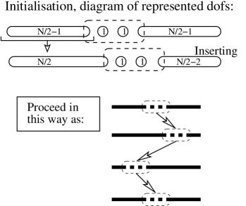
In DMRG this ’growing’ of blocks is first used in an initialization step until the superblock describes a sufficiently large system, see Fig. 2. Then an iteration is carried out to increase accuracy. Here only one side is grown, while the other is replaced by an already calculated block so that the effective size of the superblock is constant, see Fig 3.

III.2 DMRG-POD

Basically three modifications are necessary to obtain a DMRG-POD algorithm

First,

instead of a diagonalization of the superblock operator, a POD on the superblock system has to be performed. This is composed of first, a simulation of the superblock system, as defined in Eq.(22). Then the superblock correlation matrix from the generated data has to be diagonalized. This gives an orthonormal set of vectors which are the target vectors in the context of DMRG.

Second,

to each sub-block there exist not only a linear sub-block operator but also higher order operators, given by third and higher order tensors, see Eq.(17). These have to be updated in a similar way.

Third,

for the POD the initial states for the sample trajectories are crucial. The initial states are defined for the full system. They have to be projected onto the superblock system which requires all truncation matrices explicitly.

Concerning the first point, this is no great difference, since the POD (simulation and diagonalization of the correlation matrix) returns also a orthonormal set of ’relevant’ states (the POD modes) that serve as target states, as described above.

Beside the linear operator ($L$ in Eq.(1)) which is assembled identically as the superblock operator in DMRG, the higher order operators have to be a assembled also. This is principally possible, but complex. Here we use a simple trick. For all our models it is sufficient to know the component-wise squaring operator $\Omega_{i,j,k}:=\delta_{ij}\delta_{ik}$. (And in some cases the derivative operator which is linear and is also assembled like the superblock Laplace operator.) $\Omega$ is purely diagonal, so no links have to be stored and assembled. The reduction with a truncation matrix $R$ is straightforward:

$$\hat{\Omega}_{i,j,k}=\sum_{a,b,c}R_{i,a}\Omega_{a,b,c}R_{b,j}R_{c,k}$$ (29)

From this the higher order tensors can be calculated directly, e.g. for the Burgers equation

$$\hat{Q}_{\mbox{Burgers},i,j,k}:=\nu\sum_{l}\delta_{ij}\delta_{lj}\hat{D}_{x,N,l,k}$$

$$=\sum_{l}\hat{\Omega}_{j,i,l}\hat{D}_{x,N,l,k}.$$ (30)

For fourth and higher order operators this procedure is a bit memory consuming. E.g for calculating $\Phi^{3}$ it is more efficient to calculate first $\Phi_{\mbox{\scriptsize tmp}}:=\hat{\Phi}^{2}=\Omega\Phi\Phi$ and then $\hat{\Phi}^{3}=\hat{\Phi}^{2}\hat{\Phi}=\Omega\Phi_{\mbox{\scriptsize tmp}}\Phi$.

The third point is a small disadvantage, since the projection operators have all to be stored, which is not necessary in DMRG if only the energy values are of interest. However, here as well as in DMRG it is possible to expand a superblock state to a state of the original system as well as project down a system state to the superblock if all truncation matrices are stored. The down-projection of the $N$-dimensional state is in particular done by iteratively contracting the $m+1$ outermost sites of e.g. $\Phi$ with the corresponding block truncation matrix $R$. Apart from the memory requirement this is simply a book keeping problem.

It should be noted that only $m+1$ most relevant states from the POD are used as target states. Thus only $m+1$ relevant states of the superblock are optimized although it represents $2m+2$ dofs. This has to be considered in comparing the results. However, the DMRG POD is nevertheless faster than the full POD, see section V.1.

To summarize: Apart from the POD itself, which is a standard technique, no fundamental changes have to be implemented to get a DMRG-POD method from the simple toy model DMRG. The assembly of linear operators has to be performed in any case, only our method requires several operators. The assembly of the $\Omega$ operator is even more simple, since all links vanish. Reconstruction of full system states is also possible in DMRG, only it is mandatory for our method for evaluating the correct initial conditions.

IV Application

For all applications we choose a finite differencing scheme of second order accuracy, homogenous Neumann conditions at the boundaries and the explicit Euler method for the calculations. The details are given in section I, above. The boundary conditions as well as the time integration method can be chosen - more or less - arbitrarily. However, higher order finite elements in the spatial discretization lead to additional interactions between single dofs, i.e. a form of non-locality and do thereby complicate the problem. For the reduced system size always four dofs were retained. This is mainly for convenience and easy comparison. The success of the method does not depend strongly on this choice.

As explained above, we measure the quality of a reduction by the $L^{2}$-error, see Eq.(24). It has the same units as the fields $\Phi$ which are not further specified. The time units are also arbitrary. The error calculations in the following are performed in a separate program which gets the optimized bases from the various methods as input. Thus the simulation time do not have to coincide with the length of the POD simulations. Further we have chosen a different random seed for statistical initial conditions unless otherwise stated.

IV.1 Linear Diffusion

For this problem the dynamics is given by Eq.(2).

Figure 4: Reduced diffusion equation $L^{2}$-Error $E(t)$ for the analytical reduction (Fourier modes) the full POD and DMRG POD after initialization and several iterations, statistical initial condition, N=40, $h_{t}=0.001$ and $d=0.05$. The error is expressed in units of $\Phi$, for the time axis arbitrary units are employed. Note that for clarity not all data points are shown as symbols.

Figure 5: Reduced diffusion equation $L^{2}$-Error $E(t)$, identical statistical initialization. The error is expressed in units of $\Phi$, for the time axis arbitrary units are employed. Note that for clarity not all data points are shown as symbols.

The only nonzero contribution according to Eq.(1) is $L\equiv\Delta_{N}$. The eigenstates of $L$ are the sine/cosine or Fourier modes whose contributions decay over time with characteristic life-time inversely proportional to the frequency/energy. Standard DMRG can be viewed as an approximate diagonalization method for an linear operator. Therefore it is very effective to find the optimal reduction determined by the eigenstates, see Appendix VI, in the linear case. In contrast to the diagonalization, POD as well as our method depends on the initial conditions for the sample trajectories over which the averaging is carried out. Both POD approaches cannot exploit the linearity of the evolution equation. This affects the quality of the results for linear problems compared to diagonalization-based methods. Nevertheless, restriction to a few sample trajectories can also be an advantage, since sometimes the interest lies on a certain region in phase space. However, for the diffusion equation we choose normally distributed initial conditions, i.e. the field $\Phi_{0}(x_{i})$ is normally distributed. This is then also true for the Fourier modes. By this choice effectively the whole phase space will be sampled for a high enough number of realizations. This is also due to the invariance of Eq.(2) under multiplication with a constant factor.

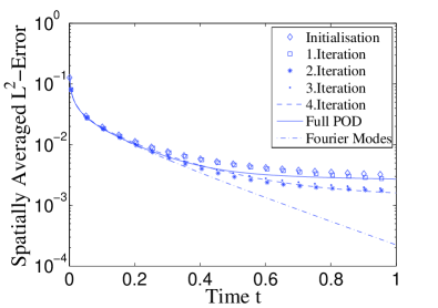
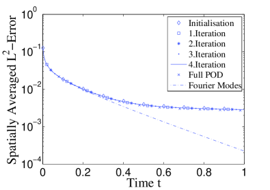
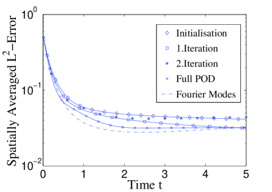
For the POD it is important to integrate over long enough times. For short times the state moves in the direction of the highest frequency modes which are decaying most rapidly. Thus POD would give the wrong relevant modes. The POD is in fact not a very appropriate tool to reduce the whole phase space of the diffusion equation. In Fig. 4 the error of the reduced fields $\hat{\Phi}$ is plotted in dependence of time. There the time step was $dt=10^{-3}$ and the diffusion constant $d=0.05$. The spatial resolution was $40$ lattice sites within the interval $[0,1]$. In each POD step as well as for the error calculation the ensemble average, compare with Eq.(25), has been averaged over $50$ realizations of the initial conditions. From this result we can state several things. First, all POD-based methods show a remaining error in the long time limit. Second, the initialization steps of DMRG POD gives already reasonable results. An improvement due to the iteration is present, too. Third, our algorithm is able to compute the optimal reduction with even higher accuracy than the full POD. The last point is only paradox on the first glance. The inaccuracy of the full POD is in this case influenced from the statistical initial conditions, in order to sample the full phase space. Within our algorithm, much more initial conditions are taken into account as the superblock POD is performed repeatedly. This leads to a better statistics. In Fig. 5 we have shown the same results but using always the same initialization for calculating all PODs (but of course not for the error calculation). It is clear that in this case, our method has no advantage over the full POD anymore. On the other hand, the results from our algorithm are not worse than that from the full system POD, which is not clear a priori.

Figure 6: Reduced Burgers equation $L^{2}$-Error $E(t)$, deterministic initial condition, N=40, $h_{t}=0.02$, $d=0.01$ and $\nu=0.1$. The error is expressed in units of $\Phi$, for the time axis arbitrary units are employed. Note that for clarity not all data points are shown as symbols.

Figure 7: Reduced Burgers equation $L^{2}$-Error $E(t)$, deterministic initial condition, N=100, $h_{t}=0.005$, $d=0.01$ and $\nu=0.1$. The inset shows the begin of the error evolution enlarged. The error is expressed in units of $\Phi$, for the time axis arbitrary units are employed. Note that for clarity not all data points are shown as symbols.

IV.2 Burgers Equation

The Burgers equation is given by Eq.(6). The discretization used here is already described above. We begin our analysis with the choice of deterministic initial condition for the calculation of all PODs. In particular it is of the form

$$\Phi(t=0,x_{i})=e^{-50(x_{i}-1)^{2}}\quad x_{i}=0\ldots 1.$$ (31)

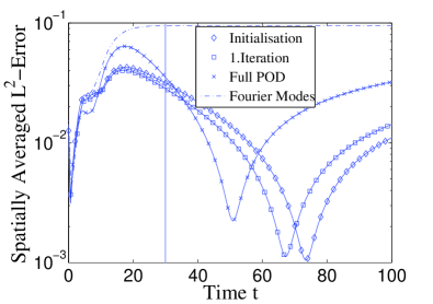
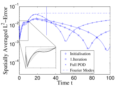
Fig. 6 and 7 show the results for the $L^{2}$-Error of the evolution. Here we have used two spatial resolutions, i.e. $N=40$ and $N=100$ nodes. The results are very similar. In contrast to the previous calculations the simulation runs for the error calculation are longer than the POD runs. The vertical line indicates the time interval of the POD runs. Here we have to state that the Fourier mode reduction is not optimal, which is not surprising as we consider a nonlinear system and a very particular region of phase space. Further, we see that the error curves show a very pronounced minimum after which the approximation seemingly breaks down. The corresponding time point lies well after the POD time-span. These minima correspond to the fact that after the passing of the wavefront the profile becomes flat. The approximations do not reproduce the average value accurately, but show a spurious drift. The passing of the reduced (flat) states by the original (flat) state creates the minima in Fig. 6.

It is remarkable that our methods yield better results than the POD within the POD time, even for the initialization. Here it should be recalled that the POD is optimal only for reconstructing the states used in the calculation. As stated above, the reconstruction of the dynamics that created these states, is a different thing as can be directly seen from our results.

We continue our analysis of the Burgers equation by considering statistical initial conditions. In contrast to the calculations for the diffusion equation we have only three randomly sampled parameters in the initial condition. It is given by a peak of various height $H$, width $W$ and position $X$. In particular it is defined by the following equation

$$\Phi(t=0,x_{i})=He^{-50W(x_{i}-X)^{2}}.$$ (32)

Here, $H$ and $W$ are normally distributed whereas $X$ is uniformly distributed.

Figure 8: Reduced Burgers equation $L^{2}$-Error $E(t)$, statistical initial condition, N=20, $h_{t}=0.01$, $d=0.05$ and $\nu=0.1$. The error is expressed in units of $\Phi$, for the time axis arbitrary units are employed. Note that for clarity not all data points are shown as symbols.

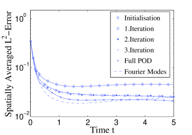
The results are shown in Fig. 8. For all methods the error reaches a plateau very quickly. The performance of the full system POD is slightly better than that of the DMRG POD. However, the errors from our approach are of the same order as from the full POD and one magnitude better than that of the Fourier mode based reduction. Also the iteration brings an improvement which reaches saturation already after the first step.

Figure 9: Reduced nonlinear diffusion equation $L^{2}$-Error $E(t)$, statistical initial condition, N=30, $h_{t}=0.03$, $d=0.01$ and $a=0.5$. The error is expressed in units of $\Phi$, for the time axis arbitrary units are employed. Note that for clarity not all data points are shown as symbols.

Figure 10: Computing time for various system sizes and approaches, obtained by the reduced Burgers equation, statistical initial condition, N=40, $h_{t}=0.005$, $d=0.01$ and $\nu=0.1$.

For deterministic initial conditions the evolution of the error is not monotonic in contrast to the case of statistical initial conditions. This is due to the fact that deterministic initial conditions can be considered more effectively by the POD. The statistical initial conditions were drawn from a three, see Eq.(32) or two, see Eq.(33), dimensional subspace which is reproduced poorly by a reduction to a 4 dimensional space, which has to consider the time evolution also.

IV.3 Nonlinear Diffusion

This system is defined by Eq.(11). As initial conditions we have chosen a front with uniformly distributed position $X$ and normally distributed height $H$:

$$\Phi(t=0,x_{i})=\frac{H}{2}\tanh((x_{i}-X)10).$$ (33)

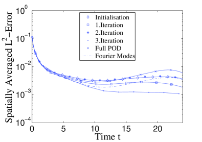
Under this conditions all methods were able to reproduce the dynamics well, see Fig. 9. Surprisingly the full POD method gave poorer results than even the Fourier mode based reduction. This is to a lower extent also true for the initialization run of the DMRG POD. The iteration lead to an improvement although the 2nd iteration gave similar results as the initialization. Further iterations again increase the accuracy, so no general statement can be made. After a fast saturation by applying the iteration procedure we observed repeatedly a decay in the quality of the results, which we attributeto the accumulation of numerical errors.

V Discussion

V.1 Computational Load

For all calculation steps, e.g. diagonalization, Gram-Schmidt orthonormalization etc., standard algorithms were applied Golub and VanLoan (1983-1996); Press et al. (1984-2006). The focus was more on a concise assessment of the new algorithm instead of an optimal solution of the toy problems. For the diagonalization of the covariance matrix, e.g. first a Householder-tri-diagonalization was performed Golub and VanLoan (1983-1996), which is an ${\mathcal{O}}(N^{3})$ algorithm. The calculation of the POD, either for the complete system or for the superblock system was performed with the same routine. This comprised the simulation as well as the diagonalization.

For a POD the simulation of the system in the time-span of interest is additionally necessary. The required computational load for this simulation is implementation dependent and is denoted with $S(\cdot)$. Within our approach the simulation and diagonalization is performed only on the superblock system. Comparing the results from Fig. 6 and  7 suggests, that the necessary number of iterations (sweeps) does not depend on the full system size $N$. If we denote the superblock size with $M$ and the number of iterations with $N_{i}$ a naive estimation of the computational load is given in table 1.

full system POD	DMRG POD
$O(N^{3})+S(N)$	$NN_{i}O(M)+S(M)$

Table 1: Naive estimation of the computational load with full system size $N$, superblock size $M$ and numbers of iterations $N_{i}$. The computational load for the simulation is denoted with $S(\cdot)$

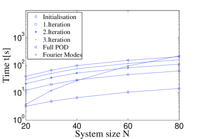
For a more quantitative analysis we have measured the time necessary to perform a full POD comprised of simulation and diagonalization. Then we did the same for the initialization of the DMRG POD algorithm including all simulation and diagonalization steps until the superblock system described the full system of dimensionality $N$, compare Fig. 2, and a first reduced basis had been calculated. We also measured the computing time for one further iteration step in the same way as for the initialization. The computing time is constant for all iteration steps so further data was extrapolated. The underlying equation was the deterministic initialized Burgers equation although the choice for an equation affects the computational load only marginally. As parameters we have chosen $h_{t}=0.005$, $d=0.01$ and $\nu=0.1$. Fig. 10 shows a logarithmic plot of the results. The DMRG POD approach shows a lower amount of computer time for the initialization step. For higher system size this holds also for the iterations. Generally the scaling with $N$ is favorable. Note, that here only the DMRG method should be assessed. For this purpose public assessable standard algorithms are sufficient, although much more effective methods could be possible. All calculations were performed on an Intel Dual Core machine, using a single CPU.

V.2 Stability

Many numerical schemes and the explicit Euler method in particular show instabilities for certain parameter ranges. For the explicit Euler method the stability condition is

$$|1+\lambda h_{t}|\leq 1,$$ (34)

where $\lambda$ is the largest eigenvalue of the generator of evolution and $h_{t}$ the size of the time step. For the Laplace operator the highest frequency component is the first to become instable while increasing $h_{t}$. The eigenvalue is $\frac{-4}{\delta x^{2}}\sin^{2}\left(\frac{\pi(N-1)}{N}\right)\approx\frac{-4}{(\delta x)^{2}}$. Consequently, we should have $h_{t}\leq\frac{(\delta x)^{2}}{2d}$, $d$ being the diffusion constant. We have performed calculation directly at this limit, see Fig. 11 and have seen no signs of instability. Although the nonlinear Burgers equation was considered, the previous point holds, since the symmetric derivative operator has no nonzero real part eigenvalues. By increasing $h_{t}$ the instability appears for all methods. These calculations were only first tests and further work is required. However, it can be assumed that in the DMRG POD calculation the instability originates only from the newly inserted nodes which correspond to the highest spatial resolution. Combined implicit-explicit methods Fryxell (1986) could be used to solve this problem.

Figure 11: Reduced Burgers equation $L^{2}$-Error $E(t)$, statistical initial condition, N=40, $h_{t}=0.00625$, $d=0.05$ and $\nu=0.1$. The error is expressed in units of $\Phi$, for the time axis arbitrary units are employed. Note that for clarity not all data points are shown as symbols.

Figure 12: Pictorial representation of the approximation.

V.3 Interpretation of the Algorithm

The various steps, necessary for a DMRG version of the Proper Orthogonal Decomposition, seem to be complex on the first glance. It is also not clear why this approach should be effective. We now shortly depict the basic idea behind this algorithm.

The DMRG algorithm decomposes the spatial domain but considers an interaction of the domains due to the superblock concept. The single blocks, together with information about interaction with neighboring blocks and the reduced operators, describe spatial regions with a higher number of nodes than the number of dofs actually retained in the block. Inserting nodes described by the full (yet already discretized) dynamics corresponds to increasing the spatial resolution locally. The surrounding blocks simulate the environment for a small subsystem with correct dynamics. In the DMRG POD algorithm now the area with high resolution is moved through the system. Thereby the parameters of superblock system, i.e. the block basis and operator matrix elements, are adapted to approximate the full system. For more graphical illustration see Fig. 12. These arguments are a bit heuristic, but until now no rigorous proof for the algorithm has be given.

V.4 Conclusion and Outlook

To summarize, we have given a demonstration of applicability for a new algorithm to calculate an approximate POD without ever simulating the full system. Our approach also makes practically no assumption on the equations that define the dynamics. The approach has been tested for linear systems where its performance was even higher than the full system POD results but considerable worse than the optimal reduction. Several nonlinear systems have been considered. For the Burgers equation the results of the full POD and our algorithm were comparable and significantly better than a Fourier mode based reduction.

Further work on this topic will include extensions to higher dimensional systems. A method for 2 and 3 dimensions is currently in progress. Further, driven systems and systems with noise shall be implemented. A closer analysis of the quality of the approximations as well as the limitations of the method has to be performed. We have access to the amount of discarded information from the discarded eigenvalues in the truncations as well as in the POD steps. This suggests an adaptive approach for the reduction.

I would like to thank Prof.F. Schmid, Prof. Ph.Blanchard and Javier Rodriguez-Laguna DE 896/1- (1/2) for discussion and the German science foundation (DFG) for support (DE 896/1-(1,2) 2004-2007).

VI Appendix

For completeness, we assess in the following the error of the reduced evolution for the linear case. For the optimal reduction we require a minimal $L^{2}$-error for the reduced field with respect to the un-reduced evolution. The full time evolution in the $N$ dimensional phase space is generated by $L$ as

$$\Phi(t)=e^{(t-t_{0})L}\Phi(t_{0}).$$ (35)

The explicit Euler algorithm approximates this by

$$\Phi(t)\approx\left(\openone+h_{t}L\right)\Phi(t_{0}).$$ (36)

We assume that all eigenvalues of $L$ are negative or zero. A positive eigenvalue would lead to an unbounded exponential growth in Eq.(35) which is unphysical. Considering only linear projections the reduction is defined by the operator $P$ which is the orthogonal projection to the relevant subspace $\mbox{Range}(P)$. $P$ can be constructed from an ONB of this space. Equivalently, it can be defined via the ONB (namely $C$) of $\mbox{Kern}(P)$ so that $P=\openone-CC^{\dagger}$.

The reduced time evolution becomes

$$\hat{\Phi}(t)=e^{(t-t_{0})PLP}P\Phi(t_{0})=e^{(t-t_{0})\hat{L}}\hat{\Phi}(t_{0}),$$ (37)

since after each (infinitesimal) time step the component within the irrelevant subspace, i.e. $\mbox{Kern}(P)$ are projected out. For a general $P$ the eigenvectors of $\hat{L}$ are not the same as for $L$, but known eigenvectors of $\hat{L}$ are always the column vectors of $C$.

VI.1 Long Time Optimised Projection

If we assume that the eigenvalues of $L$ are $\leq 0$, for long times $t\gg 1$ the time evolution operators $e^{t\hat{L}},e^{tL}$ become the projectors onto the kernels of $L$ or $\hat{L}$, respectively. In the eigenbasis $\psi^{eig}_{i}$ it is simply

$$\psi^{eig}_{i}e^{tL}\psi^{eig}_{j}=\delta_{ij}e^{t\lambda_{i}}$$ (38)

The product of the reduced evolution operator $e^{tPLP}$ and $P$ converges for long times to the projector onto $\mbox{Kern}(PLP)\cap\mbox{Range}(P)$. More explicitly this is

$$\lim\limits_{t\rightarrow\infty}e^{tL} = \left.\openone\right|_{\mbox{\small Kern}(L)},$$ (39)

$$\lim\limits_{t\rightarrow\infty}e^{tPLP} = \left.\openone\right|_{\mbox{\small Kern}(PLP)}.$$ (40)

This gives for the error

$$E_{\infty}=\lim\limits_{t\rightarrow\infty}E\Phi(t)=\left(\left.\openone\right|_{\mbox{\small Kern}(L)}-\left.\openone\right|_{\mbox{\small Kern}(PLP)}P\right)\Phi(t_{0}).$$ (41)

In the long time limit we can obtain a zero error for all initial conditions if we have

$$\mbox{Kern}(PLP)\cap\mbox{Range}(P)\equiv\mbox{Kern}(L).$$ (42)

This is achieved by requiring

$$\mbox{Kern}(L)\subset\mbox{Range}(P),$$ and (43)

$$\mbox{Range}(P)\quad L\mbox{ invariant.}$$ (44)

as we show now.

Consider a $\phi\in\mbox{Range}(P)$. Then $P\phi=\phi$ and due to the $L$-invariance of $\mbox{Range}(P)$ it is $L\phi\in\mbox{Range}(P)$ resulting in $PLP\phi=PL\phi=L\phi$. This gives for $P$ with $\mbox{Range}(P)$ being $L$-invariant

$$\mbox{Kern}(PLP)\cap\mbox{Range}(P)=\mbox{Kern}(L)\cap\mbox{Range}(P).$$ (45)

Eq.(42) can be retrieved from Eq.(45) just by requiring condition (43). Thus, in the long time limit Eq.(41) becomes identically zero.

VI.2 Short Time Optimised Projection

For short times we consider here the reduction from a $N$-dimensional to a $(N-1)$-dimensional system.For further reductions the results can be applied by iteration. The projector $P$ becomes then $P_{ij}=\openone_{ij}-c_{i}c_{j}$ where ${\bf c}$ is the removed state. In order to minimize the error for the short time evolution measured by the $L^{2}$-norm we have to minimize

$$E_{s}(t) = ||e^{tL}\phi-e^{PLP}P\phi||_{2}$$

$$\approx ||\left(\openone+tL-P-PLP\right)\phi||_{2}=||E\phi||_{2}.$$

Here we have already used an expansion in powers of $t$ and truncated after the first order terms.

Since we have no information on $\phi$, we minimize Eq.(VI.2) by using the Frobenius norm $|\cdot|_{F}$ of the error operator $E$. The Frobenius norm is consistent with the $L^{2}$-norm Golub and VanLoan (1983-1996), i.e.

$$||Ax||_{2}\leq|A|_{F}||x||_{2}\quad\forall A\in R^{n\times n},x\in R^{n}.$$ (47)

By inserting $P=\openone-C$ we get for the error operator

$$E= \openone-P+t(L-(\openone-C)L(\openone-C))$$

$$= C+t(L-L+LC+CL-CLC)$$

$$= C+t(LC+CL-CLC).$$ (48)

We assume $L$ to be symmetric, i.e. $L_{ij}=L_{ji}$. Thus $L$ has an orthonormal eigenbasis $\left\{\varphi_{i\alpha}\right\}_{\alpha=1\ldots N}$ where the columns are the eigenvectors of $L$. The eigenvalues are $\lambda_{\alpha}$ and the matrix elements of the error operator $E$ are decomposed in this basis as

$$E_{ij} = \sum\limits_{\alpha\beta}\varphi_{\alpha i}E_{\alpha\beta}\varphi_{\beta i}$$ (49)

$$= C_{ij}+t\sum\limits_{n}\left(L_{in}C_{nj}+C_{in}L_{nj}-\sum\limits_{m}C_{in}L_{nm}C_{mj}\right)$$

with

$$C_{ij} = \sum\limits_{\alpha\beta}\varphi_{\alpha i}c_{\alpha}c_{\beta}\varphi_{\beta j},$$ (50)

$$\sum\limits_{mn}C_{in}L_{nm}C_{mj} = \sum\limits_{\alpha\beta nm}\varphi_{\alpha i}c_{\alpha}c_{n}L_{nm}c_{m}c_{\delta}\varphi_{\beta j},$$ (51)

$$\sum\limits_{n}L_{in}C_{nj} = \sum\limits_{\alpha\beta n}\varphi_{\alpha n}L_{in}c_{\alpha}c_{\beta}\varphi_{\beta j},$$ (52)

$$\sum\limits_{n}C_{in}L_{nj} = \sum\limits_{\alpha\beta n}\varphi_{\alpha i}c_{\alpha}c_{\beta}L_{nj}\varphi_{\beta n}.$$ (53)

We use the orthogonality of the $\varphi_{\alpha}$, i.e.

$$\sum\limits_{i}\varphi_{\alpha i}\varphi_{\beta i}=\delta_{\alpha\beta}=\sum\limits_{i}\varphi_{i\alpha}\varphi_{i\beta}.$$ (54)

In the eigenbasis the removed degree of freedom ${\bf c}$ can be written as ${\bf\tilde{c}}$ with components

$$\tilde{c}_{i}=\sum\limits_{\alpha}\varphi_{\alpha i}c_{\alpha}\quad,\quad c_{\beta}=\sum\limits_{i\alpha}\varphi_{\alpha i}\varphi_{\beta i}c_{\alpha}=\sum\limits_{i}\varphi_{\beta i}\tilde{c}_{i}.$$ (55)

The average of $L$ in the removed state ${\bf c}$, is

$$\left<L\right>_{{\bf c}} := \sum\limits_{nm}c_{n}L_{nm}c_{m}=\sum\limits_{nmij}\varphi_{ni}\tilde{c}_{i}L_{nm}\varphi_{mj}\tilde{c}_{j}$$

$$= \sum\limits_{nij}\varphi_{ni}\tilde{c}_{i}\lambda_{j}\varphi_{nj}\tilde{c}_{j}=\sum\limits_{i}\tilde{c}_{i}^{2}\lambda_{i}$$

The matrix elements from Eq.s(50-53) become

$$C_{ij} = \tilde{c}_{i}\tilde{c}_{j},$$ (57)

$$\sum\limits_{mn}C_{in}L_{nm}C_{mj} = \tilde{c}_{i}\left<L\right>_{{\bf c}}\tilde{c}_{j},$$ (58)

$$\sum\limits_{n}L_{in}C_{nj} = \sum\limits_{\alpha n}\varphi_{\alpha i}L_{\alpha n}c_{n}\tilde{c}_{j}$$ (59)

$$= \sum\limits_{n}\lambda_{i}\varphi_{ni}c_{n}\tilde{c}_{j}$$

$$= \lambda_{i}\tilde{c}_{i}\tilde{c}_{j},$$

$$\sum\limits_{n}C_{in}L_{nj} = \sum\limits_{n}\tilde{c}_{i}c_{n}\lambda_{j}\varphi_{nj}$$ (60)

$$= \tilde{c}_{i}\tilde{c}_{j}\lambda_{j}.$$

Thus for the matrix elements of the error operator we obtain

$$E_{ij}=\tilde{c}_{i}\tilde{c}_{j}\left(1+t\left(\lambda_{i}+\lambda_{j}-\left<L\right>_{{\bf c}}\right)\right).$$ (61)

We minimize the Frobenius norm of $E$ given by

$$|E|_{F}=\sum\limits_{ij}|E_{ij}|^{2}=\sum\limits_{ij}\tilde{c}_{i}^{2}\tilde{c}_{j}^{2}\left(1+t\left(\lambda_{i}+\lambda_{j}-\left<L\right>_{{\bf c}}\right)\right)^{2}$$ (62)

for a normalized ${\bf c}$, i.e.

$$1=||c||_{2}^{2}=\sum\limits_{i}c_{i}^{2}=\sum\limits_{i}\tilde{c}_{i}^{2}.$$ (63)

Since $E$ is a linear operator it follows that $||E{\bf x}||_{2}=||{\bf x}||_{2}||E\hat{\bf x}||_{2}$ with ${\bf x}=\hat{\bf x}||{\bf x}||_{2}$. Without no restriction to $||{\bf x}||_{2}$ the zero vector would always minimize $||E{\bf x}||_{2}$. Furthermore, each lower bound $K$ for $||{\bf x}||_{2}$ will lead to the same $\hat{\bf x}$ with $||\hat{\bf x}||_{2}=K$. This is not true for the general nonlinear case as in Degenhard and guez Laguna (2002).

Incorporating this condition $|E|_{F}$ reduces to

$$|E|_{F}^{2} = 1+2t\left<L\right>_{{\bf c}}+2t\left<L\right>_{{\bf c}}-2t\left<L\right>_{{\bf c}}+t^{2}\left<L\right>_{{\bf c}}^{2}$$

$$+ 2t^{2}\left<L\right>_{{\bf c}}^{2}-2t^{2}\left<L\right>_{{\bf c}}^{2}+t^{2}\left<L\right>_{{\bf c}}^{2}-2t^{2}\left<L\right>_{{\bf c}}^{2}+t^{2}\left<L\right>_{{\bf c}}^{2}$$

$$= 1+2t\left<L\right>_{{\bf c}}+t^{2}\left<L\right>_{{\bf c}}^{2}=\left(1+t\left<L\right>_{{\bf c}}\right)^{2}$$

$$\Rightarrow|E|_{F} = \left|1+t\left<L\right>_{{\bf c}}\right|.$$ (64)

Consequently, in order to minimize $|E|_{F}$ we have to minimize $\left<L\right>_{{\bf c}}$.

The minimization itself is performed using Lagrangian multipliers for the constraint Eq.(63). The necessary condition for a minimum is

$$0 = \frac{\partial}{\partial\tilde{c}_{k}}\left(\left<L\right>_{{\bf c}}+\eta\left(1-||{\bf c}||_{2}^{2}\right)\right)$$

$$= \frac{\partial}{\partial\tilde{c}_{k}}\sum\limits_{i}\left(\tilde{c}_{i}^{2}\lambda_{i}+\eta\left(1-\tilde{c}_{i}^{2}\right)\right)$$

$$= 2\tilde{c}_{k}\left(\lambda_{k}-\eta\right).$$

This is true if either $\tilde{c}_{k}=0$ or $\eta=\lambda_{k}$. The last equation can only be true for a single value of $\lambda_{k}$. We denote the nonzero component as $\tilde{c}_{k^{\prime}}\neq 0$ and $\tilde{c}_{k}=\delta_{kk^{\prime}}\tilde{c}_{k^{\prime}}$. From Eq.(63) it follows further that $\tilde{c}_{k}=\delta_{kk^{\prime}}$.

Inserting this in Eq.(64) we obtain

$$|E|_{F}=\left|1+t\sum\limits_{k}\tilde{c}_{k}^{2}\lambda_{k}\right|=\left|1+t\lambda_{k^{\prime}}\right|.$$ (66)

For small $t$ , i.e. $t<|\lambda_{i}|^{-1}$ $\forall i$ this is clearly minimal if we choose $\lambda_{k^{\prime}}$ to be the smallest eigenvalue.

Further iterations, e.g. $n$ times, of selecting the irrelevant states remove successively the eigenstates corresponding to the $n$ lowest eigenvalues. This is due to the fact that the spaces Kern($C$) $\equiv$ Range($P$) and Range($C$) $\equiv$ Kern($P$) are by construction $L$ invariant. This also makes the iteration unambiguous, a feature that is in general not present for nonlinear problems.

Note also that since $\lambda_{i}\leq 0$ the reduced states always belong to Range($L$) as long as any remaining eigenvalue, i.e. an eigenvalue of $P_{n-1}LP_{n-1}$ is nonzero. Here, $P_{n-1}$ results from the previous reduction step. In this case the error always vanishes for long times.

Summarizing, the optimal short time projection leads to results that are not only consistent with the long time accuracy requirements, but even include them.

References

- Sirovich (1987) L. Sirovich, Quarterly of Applied Mathematics XLV, 561 (1987).
- Murray (2002) J. D. Murray, Mathematical biology (Berlin, Springer, 2002), ed.
- Lucia et al. (2004) D. Lucia, P. S. Beran, and W. A. Silva, Progress in Aerospace Sciences 40, 51 (2004).
- White (1992) S. R. White, Physical Review Letters 69, 2863 (1992).
- Burgers (1974) J. M. Burgers, The nonlinear diffusion equation (Boston, Riedel, 1974).
- Press et al. (1984-2006) W. H. Press, S. A. Teukolsky, W. T. Vetterling, and B. P. Flannery, Numerical recipes (Cambridge Univerity Press, 1984-2006).
- FitzHugh (1961) R. FitzHugh, Biophysical Journal 1, 445 (1961).
- Yanagita et al. (2005) T. Yanagita, Y. Nishiura, and R. Kobayashi, Physical Review E 71, 036226 (2005).
- Gorban et al. (2004) A. N. Gorban, I. V. Karlin, and A. Y. Zinovyev, Physica A 333 pp. 106–154 (2004).
- Steindl and Troger (2001) A. Steindl and H. Troger, International Journal of Solids and Structures 38, 2131 (2001).
- Lorenz (1956) E. N. Lorenz, Scientific report 1, Statistical forecasting Project MIT (1956).
- Berkooz et al. (1998) G. Berkooz, P. Holmes, and J. L. Lumley, Turbulence, Coherent structures, dynamical systems and symmetry (Cambridge Monographs on Mechanics, 1998).
- Rowley et al. (2003) C. W. Rowley, T. Colonius, and R. M. Murray, Physica D 189, 115 (2003).
- Noack et al. (2003) B. R. Noack, K. Afanasiev, M. Morzynski, G. Tadmore, and F. Thiele, Journal of Fluid Mechanics 497, 335 (2003).
- Bui-Thanh et al. (2003) T. Bui-Thanh, M. Damodaran, and K. Willcox, AIAA Paper 4213 (2003).
- Antoulas (2005) A. C. Antoulas, Approximation of Large-Scale Dynamical Systems (Cambridge University Press, 2005).
- Rowley (2001) C. W. Rowley, International Journal of Bifurcation and Chaos 15, 997 (2001).
- Lucia et al. (2003) D. J. Lucia, P. I. King, and P. S. Beran, Computers and Fluids 32, 917 (2003).
- White and Noack (1992) S. R. White and R. M. Noack, Physical Review Letters 68, 3487 (1992).
- White (1993) S. R. White, Physical Review B 48, 10345 (1993).
- Golub and VanLoan (1983-1996) G. H. Golub and C. F. VanLoan, Matrix Computations (Baltimore, Johns Hopkins Univ. Press, 1983-1996).
- Fryxell (1986) B. A. Fryxell, Journal of Computational Physics 63, 283 (1986).
- DE 896/1- (1/2) DE 896/1-(1/2), DFG Projekt: (2004-2007).
- Degenhard and guez Laguna (2002) A. Degenhard and J. R. guez Laguna, Journal of Statistical Physics 106, 1093 (2002).